Article

Study of a Minimally Deformed Anisotropic Solution for Compact Objects with Massive Scalar Field in Brans–Dicke Gravity Admitting the Karmarkar Condition

1
Department of Mathematics and Physical Science, College of Arts and Science, University of Nizwa, Nizwa 616, Oman
2
Department of Physics, National Defence Academy, Khadakwasla, Pune 411023, India
3
Astrophysics Research Centre, School of Mathematics, Statistics and Computer Science, University of KwaZulu-Natal, Private Bag X54001, Durban 4000, South Africa
4
Laboratory of High Energy Physics and Condensed Matter, Department of Physics, Faculty of Sciences Aín Chock, Hassan II University of Casablanca, B.P. 5366 Maarif, Casablanca 20100, Morocco
*
Authors to whom correspondence should be addressed.
Universe 2023, 9(5), 208; https://doi.org/10.3390/universe9050208
Submission received: 20 February 2023 / Revised: 9 April 2023 / Accepted: 18 April 2023 / Published: 26 April 2023
(This article belongs to the Section Cosmology)

Abstract

:
In the present paper, we focused on exploring the possibility of providing a new class of exact solutions for viable anisotropic stellar systems by means of the massive Brans–Dicke (BD) theory of gravity. In this respect, we used the decoupling of gravitational sources by minimal geometric deformation (MGD) ( e η = Ψ + β h ) for compact stellar objects in the realm of embedding class-one space-time to study anisotropic solutions for matter sources through the modified Einstein field equations. For this purpose, we used the ansatz for Ψ relating to the prominent, well-known and well-behaved Finch–Skea model via Karmarkar condition, and the determination scheme for deformation function h ( r ) was proposed via mimic requirement on radial pressure component: θ 1 1 ( r ) = p r ( r ) and matter density: θ 0 0 ( r ) = ρ ( r ) for the anisotropic sector. Moreover, we analyzed the main physical highlights of the anisotropic celestial object by executing several physical tests for the case θ 1 1 ( r ) = p r ( r ) . We have clearly shown how the parameters α , β and ω B D introduced by massive BD gravity via the MGD approach incorporating the anisotropic profile of the matter distribution have an immense effect on many physical parameters of compact bodies such as LMC X-4, LMC X-4, Her X-1, 4U 1820-30, 4U 1608-52, SAX J1808.4–658 and many others that can be fitted.

1. Introduction

The exhaustive investigation of several sets of high-precision observational data through Cosmic Microwave Background, SuperNova type Ia, Large Scale Structure, Weak Lensing, Baryon Acoustic Oscillations and so on underpins a picture wherein the Universe is spatially flat with solely about 30% of its full energy balance in the form of luminous or dark matter types. On the other hand, the nature of the remaining 70%, living in some obscure type of perplexing “dark energy”, remains a mystery, although it may be precisely portrayed by a specific kind of anti-gravitating stress. In this regard, discovering the physics of this enigmatic dark energy, leading to the present accelerated expansion of the Universe, is a crucial objective of modern physics, specifically astrophysics and cosmology.
The intensive discussion among astrophysicists and cosmologists has revealed the possibility of different new scenarios in astrophysical and cosmological research that provide various sources for the observed acceleration and even a possibility to connect it to the associated epoch of inflationary acceleration in the extremely precocious Universe. Consequently, the general relativity theory (GRT) as a bound-together portrayal of space-time and matter gives a basic insight into the astrophysical as well as cosmological phenomena.
The careful solutions of the Einstein field equations (EFEs) represent the intrinsic characteristics of self-gravitating stellar structures. In this respect, in 1916, Schwarzschild [1] found the first spherical vacuum solution which indicates the outside geometry of perfect matter distribution. Afterward, in 1939, Tolman [2] examined smooth coordinating conditions for the resulting inside solutions with the outside one and furthermore explored some accurate solutions for perfect fluid within sight of the cosmological constant. On the other hand, in 1933, Lemaitre [3] suggested that anisotropy in the interior of heavenly structures can occur due to rotational movement, phase transition, solid core or a mixture of two fluids, and so on. At this stage, various analytical solutions are available in the literature [4,5] which are physically acceptable solutions for both isotropic and anisotropic relativistic stellar objects. Recently, several researchers have taken into account the pressure via radial and tangential components to incorporate anisotropy in the configuration of celestial bodies. Herrera and Santos [6] explored the possible parameters that prompt anisotropy in spherical stellar systems in GRT. In the same spirit, Harko and Mak [7] inferred static solutions representing the anisotropic inner side of cosmic stellar structures via the anisotropy parameter. The same authors [8] show that the anisotropy is instigated in a stellar system due to the existence of a solid core. In this respect, there are several works accessible in the literature for spherically symmetric space-time with anisotropic fluid distributions that make it possible to contrast with astrophysical observations that have been derived in [9,10,11,12,13,14,15,16,17,18,19] (and the references therein).
In order to explore salient characteristics of compact objects, viz., mechanisms of stability and hydrodynamic equilibrium, causality conditions, maximum limit of the mass–radius ratio, maximum value of the superficial red-shift, the behavior of the material content via energy conditions and so on, different strategies have been proposed. One of these strategies is gravitational decoupling through the minimal geometric deformation approach, which was originally supposed as an elective way to deform Schwarzschild space-time in sight of astrophysics braneworld. It is worth noting here that this powerful approach was originally provided in 2008 by Ovalle [20] in order to draw up such analytical stellar solutions in astrophysics as well as cosmology. In this straightforward and powerful approach, an extra source is joined in the grain distribution, relying on the prerequisite that both sources solely associate with gravitation. In this regard, the system of field equations splits into two sets with lesser degrees of freedom as contrasted to the original system when we are basing it on a geometric deformation in the radial metric ingredient. The two systems are tackled separately and their corresponding solutions are joined to acquire a solution of the full system. According to this mechanism, the authors Ovalle and Linares [21] applied the MGD approach in order to calculate an interior exact solution for an anisotropic compact celestial object; they also found that their solution is compatible with the Tolman IV solution in the background of astrophysics braneworld as well as assessing the mass consequences for the compactness of self-gravitating stellar structures. Ovalle and his colleagues [22] have also employed this approach to generate three anisotropic stellar systems via the Tolman IV solution after incorporating the anisotropy impacts in the perfect fluid distribution. Otherwise, this MGD approach has been performed to cover several other subjects such as models for neutron stars [23], anisotropic-like Tolman IV solutions [24,25], anisotropic-like Tolman VII solutions [26] as well as in alternative and modified theories of gravitation, viz., f ( G ) gravity [27], Lovelock−gravity [28], f ( R , T ) gravity [29,30] and Rastall−gravity [31], among others.
On the other hand, this MGD approach has been used by Cavalcanti et al. [32] to explore the gravitational lensing singularity beyond to the GRT, and by Casadio and his collaborators [33] to find the basic stability space for Bose–Einstein condensates in gravitational structure. In sight of variable tension fluid branes, it was additionally applied to examine the corrections to dark SU(N) stellar structure evident parameters [34].
The approach of gravitational decoupling by MGD is a greatly efficient procedure to construct solutions of EFEs for self-gravitating celestial bodies. Notwithstanding, the exchange of energy and momentum among the taken-into-account sources imposes some restriction on the deformation in the radial metric component, but the temporal metric component remains unchanged, which divides the EFEs. Consequently, in order to beat this weakness, the authors of [35] altered the MGD approach by incorporating deformations in both (radial/temporal) metric functions, which is valid solely in the case when the matter is absent, as well as when the Bianchi identities corresponding to self-gravitating systems filled with fluid are also non-satisfied. Later on, the author of [36] proposed a more general form of decoupling a spherical stellar structure by incorporating deformations in radial as well as temporal metric components. The major upper hand of the extended MGD approach is that it is conceivable for all space-time areas regardless of the choice of matter distribution without imposing any restrictions. In this respect, several researchers have used this extended MGD approach in the following ways: to generate anisotropic analogs of Tolman IV [37] and Krori–Barua [38] solutions, to extend black holes in ( 3 + 1 ) - and ( 2 + 1 ) -dimensional space-times [39,40,41,42], as well as to provide anisotropic solutions in GR and modified theories [27,43,44].
It is well known that various alternative or modified theories of gravity are incorporated via modifying the Einstein–Hilbert action, which is generally used to investigate the mystery of accelerated cosmic expansion as well as the truth of the dark sector i.e., dark matter and dark energy [45]. In strong-field systems, all modified gravity theories may stray broadly from GRT; however, in weak-field systems, they are in accord with GRT. It is well remarkable that the modified gravity theories in strong-field systems may prompt a correct and suitable gravity theory. The gravitational collapse phenomenon is a noticeable paradigm of a strong-field system, so its survey in modified gravity theories has pulled numerous researchers [46,47,48,49,50]. The dynamics of the collapse are modified in the case where we consider the modeling of the self-gravitational fluid distribution in generalized theories of gravity, which in turn uncovers the modification concealed in the fashioning of the Universe structure.
The Brans–Dicke (BD) theory of gravity [51,52] is the most natural suitable generalization of GRT and has been widely investigated in different astrophysical and cosmological aspects over the past decades. Their generalization is achieved by including Dirac perceptions in a scalar-tensor theory i.e., the gravitational field is interceded by the scalar field ϕ as well as the curvature due to geometric part i.e., Ricci scalar. BD gravity holds a constant coupling parameter ω B D , well known as the scalar field coupling, which can be tuned to fit the perceptions [51,52,53] and also integrates a massless scalar field φ ( t ) = 1 / G ( t ) to analyze the involvement of the Universe. The BD coupling parameter ω B D has been proven by a radar synchronization experiment which confirms that BD gravity is compatible with all observational tests and solar system experiments for | ω B D | > 4 × 10 4 [54,55]. On the other hand, this marvelous theory provides suitable solutions to numerous cosmic issues and also clarifies radiation-matter transition via combining observational data such as the two-degree galaxy redshift survey [56] as well as cosmic microwave background data from WMAP, VSA and CBI, which gives a broad scope of deviation from GRT [57,58,59]. We would also like to remark on recent investigations on testing BD theory and on endeavors at moderating the tensions employing specific potentials in the BD frame, see e.g., [60,61,62]. There are also tests on BD gravity with screening via scalar gravitational-wave memory, in which the author of [63] assumes that the Sun’s Vainshtein mechanism does not influence the scalar field profile generated by the distant compact celestial body and they have shown that the scalar memory effect provides a strong technique for testing BD gravity with the Vainshtein mechanism. Moreover, Sharif and his collaborators have investigated self-gravitating objects in the context of Brans–Dicke gravity [64,65,66,67].
The naturalistic systems of compact celestial bodies have widely been interpreted in scalar-tensor theories. In this regard, Ramazanoglu and Pretorius [68] investigated the allowable range taking into account the mass and scalarization of neutron stars via dispensing a mass to the scalar field. The authors of [69,70] studied how the dynamics or structure of slowly and rapidly rotating neutron stars deviate from the GRT celestial model in sight of a massive scalar field due to the most significant moment of inertia. In Ref. [71], the authors studied a certain class of scalar-tensor theories with a massive scalar field by considering a quartic self-interaction term in the potential for analyzing the comportment of static and slowly rotating neutron stars. The same authors [72] examined the impacts of a self-interacting massive scalar field on the moment of inertia and compactness of slowly rotating neutron stars by using diverse equations of state.
The coupling functions of the BD theory with a massive scalar field, which is allowed by observation, may differ significantly from those in the massless scenario, as we noted previously. Due to this occurrence, we typically come to the conclusion that anisotropic compact stellar systems with massive scalar fields could, on average, have slightly unusual topologies and properties when compared to their homologs in the massless scenario. In light of this purpose, we explore the possibility of providing exact solutions by using the decoupling of gravitational sources across MGD for viable compact stars in massive BD gravity admitting the “Karmarkar condition”.
This paper has been organized as follows: after an exhaustive introduction in Section 1, the suitable BD theory under gravitational decoupling formalism is laid down in Section 2. The basic stellar equations and the MGD approach in massive BD gravity theory are introduced in Section 3. In Section 4 and Section 5, we provide a procedure for a space-time to be embedding class-one and match the interior solution to an exterior Schwarzschild line element, respectively. The physically and mathematically adequate solutions to the modified Einstein field equations through the MGD approach with the mimic requirement on matter density and radial pressure component for anisotropy in the context of massive BD gravity are derived in Section 6. Next, in Section 7, we give the physical properties of the anisotropic stellar structure in massive BD gravity via several physical and mathematical tests. Finally, in Section 8, the conclusions are reported.

2. BD Theory under Gravitational Decoupling Formalism

In order to present the BD theory under gravitational decoupling formalism, we introduce a modified complete action in this theory that is given by
S = 1 16 π R φ ω B D φ i i φ L ( φ ) g d 4 x + L m g d 4 x + β L θ g d 4 x .
Here, R is the Ricci scalar while L m and L θ denote the matter Lagrangian density and Lagrangian density for a new sector, respectively, which have been coupled by constant β , known as the coupling constant. However, L ( φ ) denotes a non-zero scalar field. As usual, the symbol g stands for the determinant of the metric g μ ν . In this connection, the two Lagrangian density functions L m and L θ are related to the stress-energy tensor as
T μ ν = 2 g δ ( g L m ) δ g μ ν ,
θ μ ν = 2 g δ ( g L θ ) δ g μ ν .
Since Lagrangian density depends solely on the metric tensor g μ ν , then Equations (2) and (3) which yield the expressions for stress-energy tensors are expected to be of the form
T μ ν = g μ ν L m 2 L m g μ ν ,
θ μ ν = g μ ν L θ 2 L θ g μ ν .
The modified complete action (1) for the BD gravity theory may be varied with regard to metric tensor g μ ν , in order to benefit the general modified field equations as follows
R μ ν 1 2 g μ ν R = 8 π φ T μ ν + β θ μ ν + 1 φ [ φ , μ ; ν g μ ν φ + ω B D φ φ , μ φ , ν g μ ν φ , δ φ , δ 2 L ( φ ) g μ ν 2 ] .
Here, the □ represents the d’Alembert operator and it is defined as
φ = T m + Θ 3 + 2 ω B D + 1 3 + 2 ω B D φ d L ( φ ) d φ 2 L ( φ ) ,
where T m and Θ are the trace of the stress-energy tensor T i j and θ i j , respectively, and
T m = g i j T i j , Θ = g i j θ i j ,
The inner geometry of compact stellar objects is absolutely represented by a static spherically symmetric metric in Schwarzschild-like coordinates ( t , r , θ , ϕ ) as follows
d s 2 = e ξ ( r ) d t 2 e η ( r ) d r 2 r 2 ( d θ 2 + sin 2 θ d ϕ 2 ) .
Here, e ξ ( r ) and e η ( r ) represent the metric functions of an astrophysical stellar object. Moreover, all throughout this work, we use the geometrized relativistic units as { G = c = 1 } and the positive signature { + , , , }. In this respect, we examine the physical highlights of the astrophysical stellar object with anisotropic distribution identified by the accompanying stress-energy tensor
T μ ν = ( ρ ^ + p ^ t ) u μ u ν p ^ t g μ ν + ( p ^ r p ^ t ) v μ v ν .
Here, ρ ^ , p ^ r and p ^ t are the matter density, radial pressure and tangential pressure for anisotropic matter distribution, respectively, and the covariant ingredient u ν is the 4-velocity with the normalization condition u μ u μ = 1 and u ν μ u μ = 0 .

3. Basic Stellar Equations and the Minimal Geometric Deformation (MGD) Approach in BD Gravity Theory

3.1. Basic Stellar Equations in BD Gravity Theory

For a physically realistic astrophysical stellar system with spherical symmetry, the combination of equations expressed in (6)–(9) and (10) provides the following differential equations:
8 π φ ρ ^ + β θ 0 0 + 1 φ f 0 0 ( φ ) = e η η r 1 r 2 + 1 r 2 ,
8 π φ p ^ r β θ 1 1 1 φ f 1 1 ( φ ) = e η ξ r + 1 r 2 1 r 2 ,
8 π φ p ^ t β θ 2 2 1 φ f 2 2 ( φ ) = e η 2 ( ξ + ξ 2 2 + ξ η r ξ η 2 ) ,
where prime indicates the derivatives with regard to the radial coordinate, r. Moreover, the scalar tensor constituents f 0 0 ( φ ) , f 1 1 ( φ ) and f 2 2 ( φ ) can be expressed in terms of ξ and η , which are explicitly given by
f 0 0 ( φ ) = e η φ + 2 r η 2 φ + ω B D 2 φ φ 2 e η L ( φ ) 2 ,
f 1 1 ( φ ) = e η 2 r + ξ 2 φ ω B D 2 φ φ 2 e η L ( φ ) 2 ,
f 2 2 ( φ ) = e η φ + 1 r η 2 + ξ 2 φ + ω B D 2 φ φ 2 e η L ( φ ) 2 .
Nevertheless, from the expressions (6) and (9), we acquire,
φ = e η 2 r η 2 + ξ 2 φ ( r ) + φ ( r ) ,
Taking into account Bianchi Identity, the system of equations according to BD gravity theory fulfill the accompanying preservation equation
ξ 2 ( ρ ^ + p ^ r ) p ^ r + 2 r ( p ^ t p ^ r ) + [ β ξ 2 ( θ 0 0 θ 1 1 ) + β ( θ 1 1 ) + 2 β r ( θ 1 1 θ 2 2 ) ] + 1 8 π [ ξ 2 ( f 0 0 ( φ ) f 1 1 ( φ ) ) + f 1 1 ( φ ) + 2 r f 1 1 ( φ ) f 2 2 ( φ ) ] = 0 .
Furthermore, the mass function for the interior stellar structure can be formulated as
m ( r ) = r ( 1 e η ) 2 = 4 π ρ ^ + β θ 0 0 + f 0 0 ( φ ) 8 π r 2 φ d r .

3.2. Gravitational Decoupling by the Minimal-Geometric-Deformation (MGD) Approach

The system of equations given in (11)–(13) are a profoundly non-linear ensemble of equations. Along these lines, we shall apply the MGD method to deal with the non-linear system of Equations (11)–(13) divided into two subsystems of equations. In light of this non-linear system, let us take into account the grain anisotropic fluid solution { Φ , Ψ , ρ , p r , p t } by fixing the coupling constant β to zero, in order that the canonical metric (9) be appointed as,
d s 2 = e Φ ( r ) d t 2 d r 2 Ψ ( r ) r 2 ( d θ 2 + sin 2 θ d ϕ 2 ) .
Here, Ψ ( r ) = 1 2 m ^ / r represents the typical term of the mass function. Currently, in order to observe the θ -sector effects arising from the new sector θ μ ν in the non-linear system of Equations (11)–(13), we need to include the coupling parameter β within the anisotropic fluid distribution. In this way, so as to include the effects of the gravitational source θ μ ν in an anisotropic stellar system, we take into consideration the geometric deformation functions Φ and Ψ , which are given as follows:
Φ ξ = Φ + β g
Ψ e η = Ψ + β h ,
where h is the deformation linked to the constituent of the radial metrics, and g is the deformation linked to the constituent of the temporal metrics. It is worth mentioning here that the deformations expressed in (21) and (22) are absolutely radial functions; this attribute guarantees the spherical symmetry of the stellar solution. The expected MGD strategy identifies with set h = 0 or g = 0 ; for this circumstance the deformation will be carried out uniquely on the radial ingredient, surviving the temporal one unchanged, viz., g = 0 . Hence, in this regard, we obtain
Ψ ( r ) e η ( r ) = Ψ ( r ) + β h ( r ) ,
which is well known as the MGD (Minimal Geometric Deformation). Now, using this MGD approach defined in Equation (23), it is clear to observe that the non-linear system of Equations (11)–(13) divides into two systems of equations. Consequently, the first equations system is identified as follows:
1 φ 8 π ρ ^ + f ˜ 0 0 ( φ ) = Ψ r Ψ r 2 + 1 r 2 ,
1 φ 8 π p ^ r f ˜ 1 1 ( φ ) = Ψ ξ r + 1 r 2 1 r 2 ,
1 φ 8 π p ^ t f ˜ 2 2 ( φ ) =   Ψ 4 2 ξ + ξ 2 + 2 ξ r + Ψ 4 ξ + 2 r ,
it is clear that these results correspond to β = 0 , which implies that the fluid matter distribution is purely anisotropic. Hence, from now on, we refer to the system of Equations (24)–(26) known as the standard Einstein’s system in BD gravity theory. Moreover, we can establish straightforwardly the amounts of matter density, pressures (radial and tangential), viz., ρ ^ , p ^ r , and p ^ t , respectively, in terms of gravitational potentials ξ and Ψ from expressions (24)–(26). Here, f ˜ 0 0 ( φ ) , f ˜ 1 1 ( φ ) and f ˜ 2 2 ( φ ) are explicitly indicated as
f ˜ 0 0 ( φ ) = Ψ φ + 2 φ r + ω B D 2 φ φ 2 + Ψ 2 φ L ( φ ) 2 ,
f ˜ 1 1 ( φ ) = Ψ 2 r + ξ 2 φ ω B D 2 φ φ 2 L ( φ ) 2 ,
f ˜ 2 2 ( φ ) = Ψ φ + 1 r + ξ 2 φ + ω B D 2 φ φ 2 + Ψ 2 φ L ( φ ) 2 .
The BD gravity system (24)–(26) fulfill the accompanying preservation equations,
ξ 2 ( ρ ^ + p ^ r ) p ^ r + 2 r ( p ^ t p ^ r ) + 1 8 π [ ξ 2 ( f ˜ 0 0 ( φ ) f ˜ 1 1 ( φ ) ) + f ˜ 1 1 ( φ ) + 2 r f ˜ 1 1 ( φ ) f ˜ 2 2 ( φ ) ] = 0 .
Now, in order to establish the usual mass function, we use the definition of Ψ = 1 2 m ^ ( r ) r , which leads to the following relation:
m ^ ( r ) = 0 r 1 2 φ 8 π ρ ^ ( r ) + f ˜ 0 0 ( φ ) r 2 d r
where m ˜ represents the mass function for the seed space-time.
Now, the second equations system, dubbed as the quasi-Einstein system in BD gravity theory, is identified in the case where we activate the coupling constant β in the system. In this connection, we obtain
1 φ 8 π θ 0 0 + F 0 0 φ = h r h r 2 ,
1 φ 8 π θ 1 1 + F 1 1 φ = h ξ r + 1 r 2 ,
1 φ 8 π θ 2 2 + F 2 2 φ = h 4 2 ξ + ξ 2 + 2 ξ r h 4 ξ + 2 r .
where
F 0 0 φ = h φ + 2 φ r + ω B D 2 φ φ 2 + h 2 φ ,
F 1 1 φ = h 2 r + ξ 2 φ ω B D 2 φ φ 2 ,
F 2 2 φ = h φ + 1 r + ξ 2 φ + ω B D 2 φ φ 2 + h 2 φ .
Moreover, the corresponding preservation equations related to the equations system (32)–(34) give,
ξ 2 ( θ 0 0 θ 1 1 ) + d θ 1 1 d r 2 r ( θ 2 2 θ 1 1 ) + 1 8 π [ ξ 2 ( F 0 0 ( φ ) F 1 1 ( φ ) ) + F 1 1 ( φ ) + 2 r F 1 1 ( φ ) F 2 2 ( φ ) ] = 0 .
Furthermore, we notice that the linear combination of both preservation equations given in (30) and (38) with regard to coupling constant β provides the preservation equation for the full system, which is expressed in (18).
Actually, it is significant to note that, from now onward, we will describe the full physical parameters for the matter density, radial and tangential pressures as follows:
ρ ( r ) = ρ ^ ( r ) + β θ 0 0 ( r ) ,
p r ( r ) = p ^ r ( r ) β θ 1 1 ( r ) ,
p t ( r ) = p ^ t ( r ) β θ 2 2 ( r ) ,
where ρ , p r and p t are physical quantities already defined above. Then again, the physical amount, namely, the anisotropy parameter ( Δ ) can be performed by the expressions addressed in (40)–(41), read as
Δ = ( p ^ t p ^ r ) + β θ 1 1 θ 2 2 .
Presently, the internal astrophysical stellar geometry for the assisting MGD system may be specified by the accompanying metric,
d s 2 = e ξ ( r ) d t 2 1 2 m ( r ) r 1 d r 2 r 2 ( d θ 2 + sin 2 θ d ϕ 2 ) .
Here, m ( r ) characterizes the inward mass of the MGD system, which can be read as follows:
m ( r ) = r 2 2 m ^ ( r ) r β h ( r ) .
On the other hand, it is worth mentioning here that, throughout in our study, we take the following form of the scalar function field L ( φ ) as follows:
L ( φ ) = 1 2 m φ 2 φ 2 ,
where m φ represents the mass of the scalar field and φ is the scalar function which is defined as φ = α e n ξ ( r ) [73] with α and n being two constants.
As mentioned above, our objective is to find the solution using gravitational decoupling. As we know, the MGD technique allows obtaining the solution beyond the chosen gravity. Furthermore, the MGD approach divides the original system into two parts: the first system corresponds to pure Brans–Dicke gravity while the second system is due to gravitational decoupling. We have assumed that the internal structure of the first system is made of anisotropic fluid matter distribution rather than isotropic matter distribution. Therefore, we need two extra conditions to solve the first system. Due to this reason, we are interested in the embedding class-one condition (Karmarkar condition) along with the radial metric function corresponding to the Finch–Skea model to close the first system, while the second system is solved by using the mimic constraints approach. Finally, we the solution of the original system after combining the solutions of both systems, which is the generalization of the embedding class-one solution beyond the Brans–Dicke gravity. The procedure for the embedding class-one condition is discussed in next section.

4. Procedure for a Space-Time to Be Embedding Class-One

In 1925, Eisenhart [74] presented that an implanting class-one space [ n + 1 ]-D space V [ n + 1 ] can be carried out into a [ n + 2 ]-D pseudo-Euclidean space E [ n + 2 ] , which can be characterized by a [ n + 1 ]-D space V [ n + 1 ] if there remains a symmetric tensor a [ m n ] which satisfies the associated Gauss–Codazzi equations as follows:
R m n p q = 2 e a m [ p a q ] n 0 = a m [ n ; p ] Γ [ n p ] q a m q + Γ m [ n q a p ] q ,
where R m n p q and a m n are the Riemann curvature tensor and the coefficients of the second-order differential form, respectively, as well as e = ± 1 . In 1921, Kasner [75] provided that Schwarzschild’s vacuum may be submerged into 6-D pseudo-Euclidean space by a progression of coordinate transformations. This implies that the Schwarzschild outside is of class two. In the same spirit, in 1975, Gupta and Goel [76] also gave a 6-D implanted Euclidean space-time, which is specified below,
z 1 = k e ξ / 2 cosh t k , z 2 = k e ξ / 2 sinh t k , z 3 = f ( r ) , z 4 = r sin θ cos ϕ , z 5 = r sin θ sin ϕ , z 6 = r cos θ ,
which is used to transform a generalized 4-D space-time (9) into 6-D pseudo-Euclidean space, viz.,
d s 2 = ( d z 1 ) 2 + ( d z 2 ) 2 ( d z 3 ) 2 ( d z 4 ) 2 ( d z 5 ) 2 ( d z 6 ) 2 ,
with [ f ( r ) ] 2 = ( 1 Ψ ) Ψ + 1 4 k 2 e ξ ξ 2 . This also necessitates that the 4-D metric (9) may be actualized in 6-D Euclidean space; notwithstanding, there subsists a possible situation where ( d z 3 ) 2 = [ f ( r ) ] 2 = 0 , then the 6-D Euclidean space (45) may be reduced to 5-D pseudo-Euclidean space. This is possible only if
[ f ( r ) ] 2 = ( 1 Ψ ) Ψ + 1 4 k 2 e ξ ξ 2 = 0 ,
or
1 Ψ = 1 + k 2 4 ξ 2 e ξ .
The important condition (47) is equivalent to the embedded class-one solution (recognized as the Karmarkar condition), which fulfills a necessary condition that was originally determined by Karmarkar [77] with the help of Riemann tensor components as
R 1010 R 2323 = R 1212 R 3030 + R 1220 R 1330 .
In 1981, Pandey and Sharma [78] caused to notice the way that the Karmarkar condition is the only significant condition required to transform into a class-one; they found the satisfactory condition as R 2323 0 . Subsequently, the basic and suitable condition to be a class-one is one which satisfies simultaneously the Karmarkar and Pandey–Sharma conditions. Thus, in terms of the gravitational potential functions, the condition expressed in (48) can be written as
Ψ Ψ ( Ψ 1 ) = 2 ( ξ + ξ 2 ) ξ 2
in which, during integration, we obtain the g 00 gravitational potential function as
e ξ = A + B 1 Ψ 1 d r 2 .
while A and B are two integration constants. One should consistently remember that there is no class-one vacuum outside, as the static Schwarzschild’s vacuum is previously a class-two solution.

5. Exterior Space-Time: Junction Conditions

Junction conditions play a crucial and important role in the study of compact stellar structures which are bounded stellar objects by joining their interior and exterior space-time at the surface Σ in a smooth way. In this respect, we can find all the constant parameters involved in the system. The space-time corresponding to the interior solution for field Equations (11)–(13) is expressed by Equation (42). Therefore, the exterior space-time is considered to be an empty space-time i.e., the exterior Schwarzschild solution which is given explicitly as
d s + 2 = 1 2 M r 1 d r 2 r 2 ( d θ 2 sin 2 θ d ϕ 2 ) + 1 2 M r d t 2 ,
where M represents the stellar mass of the star. For analyzing the physical aspects, we need to generate a connection between the inner and outer geometries of celestial objects, which should be satisfied with the smoothness and continuity for inner and outer space-times at the hypersurface Σ ( f = r R = 0 , where R is a radius). For this purpose, the following conditions should be met at the boundary surface Σ ,
[ d s 2 ] Σ = [ d s 2 + ] Σ , [ K i j ] Σ = [ K i j + ] Σ ,
[ Φ ( r ) ] Σ = [ Φ ( r ) + ] Σ , [ Φ ( r ) ] Σ = [ Φ ( r ) + ] Σ .
1 Here, K i j denotes the curvature, whereas the subscripts − and + symbolize the interior and exterior solutions, respectively. Now, we use the continuity of the first fundamental form i.e., [ d s 2 ] Σ =0, and we will still find for any function F ( r ) ,
[ F ] Σ F ( r R + ) F ( r R ) F + ( R ) F ( R ) .
It is worthwhile to mention that this condition supplies us g r r ( R ) = g r r + ( R ) and g t t ( R ) = g t t + ( R ) . Moreover, the second fundamental form, viz., K i j , which is equivalent to the O Brien and Synge [79] junction condition at the hypersurface Σ , must be satisfied by the space-time (7). This condition denotes that radial fluid pressure p r vanishes at a certain radius r = r Σ , which is expressed as
[ p r ( r ) ] Σ = 0 p ^ r β θ 1 1 ( r ) Σ = 0 .
This requirement establishes the size of the celestial object i.e., the radius R, which implies that the material substance is restricted within the interior of the sector 0 r R , which indicates that its exterior sector does not contain any matter. Moreover, the BD scalar field Φ relating to the empty Schwarzschild solution was determined according to the procedure addressed in [80]. Now, considering τ and τ + as the inner and outer space, respectively, the line element for hypersurface is defined in terms of the proper time boundary γ as
d s 2 = d γ 2 R 2 ( d θ 2 + sin 2 θ d ϕ 2 ) .
The extrinsic curvature corresponding to the boundary Σ is given as follows:
K i j ± = m k ± 2 y ± k n i n j m k ± Γ q l k y ± q n i y ± l n j
where n i and m k ± denote the coordinates in the boundary Σ and the 4-velocity normal to Σ , respectively. Here, the components corresponding to the 4-velocity are defined in terms of the coordinates ( y ± i ) of τ ± as
m k ± = ± d f d y k | g q l d f d y q d f d y l | 1 / 2 with m k m k = 1 .
Further, the unit normal vectors for the inner and outer areas can be defined as
m k = 0 , e η / 2 , 0 , 0 , and m k = 0 , 1 2 M r 1 / 2 , 0 , 0 .
Now, considering the Schwarzschild space-time (51) and using the line elements from Equations (7) and (56), we can write
d t d γ Σ = e ξ / 2 Σ = 1 2 M r 1 / 2 Σ .
where [ r ] Σ = R . The non-zero components corresponding to the curvature, K i j , can be achieved by using expression (59) as
K 00 = ξ 2 e η / 2 Σ , K 22 = 1 sin 2 θ K 33 = r e η / 2 Σ , K 00 + = M r 2 1 2 M r 1 / 2 Σ , K 22 + = 1 sin 2 θ K 33 + = r 1 2 M r 1 / 2 Σ .
By using the junction condition [ K 22 ] Σ = [ K 22 + ] Σ with [ r ] Σ , we obtain the component of the radial space-time as follows:
e η ( R ) = 1 2 M R .
Plugging this radial gravitational component into the matching condition [ K 00 ] Σ = [ K 00 + ] Σ provides
ξ ( R ) = M R 2 1 2 M R 1 .
On the other hand, in principle, the θ -sector may create some modification in outer space-time and matter content. As such, the explicit expression for Equation (55) can be given by
p ^ r ( R ) β ( θ 1 1 ) ( R ) = β ( θ 1 1 ) + ( R ) ,
where p ^ r ( R ) refers to the radial pressure with respect to the inside matter distribution when β = 0 . The above condition (63) describes a second fundamental form related to the Einstein field equations expressed explicitly by Equation (6). Now, the formula expressed in (63) with the help of the value of ( θ 1 1 ) ( R ) for the interior space-time via Equation (33) comes out to be
β h 8 π φ ξ r + 1 r 2 + 2 r + ξ 2 φ ω B D 2 φ φ 2 r = R + p ^ r ( R ) = β ( θ 1 1 ) + ( R ) ,
where ξ r ξ and Σ represent the boundary of the celestial configuration r = R . Presently, we employ Equations (33), (61) and (62) into Equation (64) in order to find the ( θ 1 1 ) + ( R ) expressed in Equation (64) for the exterior space-time, leading to
p ^ r ( R ) + β h 8 π φ ξ r + 1 r 2 + 2 r + ξ 2 φ ω B D 2 φ φ 2 r = R = β h Σ * 8 π [ φ Σ 2 M R 2 R 2 M + 1 R 2 ω B D 2 φ Σ φ Σ 2 + 2 R + M R R 2 M φ Σ ] .
Here, h Σ * and φ Σ are two functions signifying the geometric deformation function and scalar function, respectively, for the outside Schwarzschild line element (51) at the boundary r = R of the celestial astrophysical structure due to the new sector θ i j . It should be noted that, if the outer space-time is represented by the Schwarzschild vacuum solution given in (51), at this stage, we should put h Σ * = 0, in order to obtain the final form of Equation (65), which can be derived as follows:
p ^ r ( R ) + β h ( R ) 8 π [ φ ( R ) ξ ( R ) R + 1 R 2 ω B D 2 φ ( R ) φ 2 ( R ) + 2 R + ξ ( R ) 2 φ ( R ) ] = 0 ,
which is identical to
p ^ r ( R ) β θ 1 1 ( R ) = 0 p r ( R ) = 0 .
This condition (66) or (67) establishes the size of the compact celestial body. In view of this relevant condition, we have discovered an important result that anisotropic radial pressure vanishes at the surface, which is desired for the equilibrium of a celestial object in the original Schwarzschild solution.
Finally, we want to mention that conditions (60)–(62) and (67) describe the primary and adequate conditions to establish all the constants present in the stellar system.

6. Minimally Deformed Anisotropic Solution: Mimic Constraint Approach

As the modified Einstein field equations given in (11)–(13) are divided into two subsystems according to the MGD method, the first subsystem corresponds to the field equations given in (24)–(26) with five unknown parameters { Ψ , ξ , ρ , p r , p t } for the seed solution in BD gravity with respect to the stress-energy tensor T μ ν m , whereas the second subsystem corresponds to the field equations expressed in (32)–(34) which examine the solution of new θ -sector, which basically consists of four unknown parameters { h ( r ) , θ 0 0 , θ 1 1 , θ 2 2 } . In this regard, if the first subsystem generally provides an achievable solution for anisotropic distribution, then this leads directly to the absolute evaluation of the unknown parameters of the second subsystem. In effect, for solving the system of equations via the MGD approach, we need to use the well-known embedding class-one condition to reduce the degree of freedom. Now, we take into account the ansatz for Ψ related to a well-defined notable Finch–Skea model and execute a well-known embedding class-one condition (50). Hence, we obtain the accompanying seed space-time, so-called embedding class-one seed space-time, as
d s 2 = A + a B 2 r 2 2 d t 2 d r 2 ( 1 + a r 2 ) r 2 ( d θ 2 + sin 2 θ d ϕ 2 ) .
At this stage, Ψ = 1 / ( 1 + a r 2 ) and ξ = ln A + a B 2 r 2 2 can describe the solution of the equations system (24)–(26) in the context of the BD gravity theory. Presently, in order to close the second subsystem with the new θ -sector, we necessitate the deformation function indicated by h ( r ) . Since there are diverse ways to obtain the deformation function, however, it ought to be satisfied with some fundamental prerequisites so as to be a permissible system with respect to the physical and mathematical points of view. In such a manner, a straightforward and comfortable depiction of the geometric deformation function f ( r ) [28,81,82] ought to be satisfied with these fundamental necessities or only involve oneself in the ingredients of θ -sector with a linear, polytropic or barotropic equation of state. Here, we will adopt the well-known methodology, specifically, the Mimic requirement method:
(A)
Mimic requirement on the radial pressure component of the anisotropic sector, viz., ( θ 1 1 = p r ),
(B)
Mimic requirement on the density of the anisotropic sector, viz., ( θ 0 0 = ρ ).
It is mentioned that both approaches are mainly used to determine the deformation function (h). The mimic-to-pressure constraint approach i.e., θ 1 1 = p r involves a deformation function (h) that is free from the derivative. This approach directly determines the expression for h ( r ) without any integration, while the mimicking of density constraint i.e., θ 1 1 = p r procedure provides a differential in the differential equation in the deformation function (h), whose solution depends on the seed solution. The second approach enhances the total mass of the object.

6.1. Mimic Requirement on Radial Pressure Component for Anisotropy

Here, in order to obtain a physically and mathematically adequate solution, we perform the radial pressure component expressed in Equation (25) and imitate its relationship with the anisotropic area given by Equation (33) in order to close system of Equations (32)–(34). In this scenario, we can obtain
θ 1 1 ( r ) = p ^ r ( r ) .
This necessity derives that the stress-energy tensor for the seed solution is associated with the anisotropy in a radial direction. This implies that Equations (25) and (33) are equivalent. In this way, we determine the formula for the deformation function h ( r ) , which takes the following forms:
h ( r ) = Ψ φ 2 r 2 ω B D Ψ r φ φ ( 4 + ξ r ) + f 11 ( r ) 2 φ 2 ( 1 + ξ r ) + φ φ r ( 4 + ξ r ) φ 2 r 2 ω B D .
where, f 11 ( r ) = φ r 2 L ( φ ) 2 φ 2 ( Ψ 1 + Ψ ξ r ) .
Then, the minimally deformed radial gravitational potential e η has taken its final form, which is expressed explicitly as
e η = Ψ + β Ψ φ 2 r 2 ω B D Ψ r φ φ ( 4 + ξ r ) + f 11 ( r ) 2 φ 2 ( 1 + ξ r ) + φ φ r ( 4 + ξ r ) φ 2 r 2 ω B D .
Now by combining Equations (44) and (68) into Equations (70) and (71), we obtain
h ( r ) = r 2 [ H 1 ( r ) + H 2 ( r ) ] 4 n + 1 ( 1 + a r 2 ) [ 4 A 2 H 3 ( r ) ] ,
e η = r 2 [ H 1 ( r ) + H 2 ( r ) ] 4 n + 1 ( 1 + a r 2 ) [ H 3 ( r ) 4 A 2 ] + 1 1 + a r 2 ,
where,
H 1 ( r ) = 4 A 2 α m φ 2 ( 2 A + a B r 2 ) 2 n 4 a A B [ 2 3 + 2 n + 4 2 + n n α m φ 2 r 2 ( 2 A + a B r 2 ) 2 n ] + 4 a 3 / 2 A B r 2 × [ 4 1 + n + α m φ 2 r 2 ( 2 A + a B r 2 ) 2 n ] , H 2 ( r ) = a 2 B 2 r 4 [ 4 1 + n + α m φ 2 r 2 ( 2 A + a B r 2 ) 2 n ] + a { 4 A 2 [ 4 1 + n + α m φ 2 r 2 ( 2 A + a B r 2 ) 2 n ] + B 2 r 2 × [ 4 2 + n 4 3 + n n + α m φ 2 r 2 ( 2 A + a B r 2 ) 2 n + 2 5 + 2 n n 2 ω B D ] } . H 3 ( r ) = 4 a A B ( 3 + 4 n ) r 2 + a B 2 r 4 ( 5 + 16 n 8 n 2 ω B D ) .
Now we can determine the expressions for θ -sector components directly from Equations (32)–(34), namely θ 0 0 , θ 1 1 and θ 2 2 after plugging the deformation function h ( r ) . In this situation, we can obtain
p r ( eff ) = ( 1 β ) p ^ r ( r )
p t ( eff ) = p r ( eff ) + Δ eff ,
However, Equation (39) provides the explicit expression for effective matter density, viz., ρ ( eff ) as,
ρ ( eff ) = ρ ^ ( r ) + β θ 0 0 .
This mimic constraint procedure suggests that the deformed gravitational potential function e η can be determined explicitly, due to the fact that the condition expressed in Equation (71) does not contain any integral term. On the other hand, the energy density ρ ^ ( r ) , radial p ^ r ( r ) and tangential p ^ t ( r ) pressures for the seed solution are already given by Equations (24)–(26), respectively. Now, after applying the boundary conditions (60)–(62), we obtain
A + a B 2 R 2 = 1 2 M R ,
a B R = 2 M R 2 ,
1 1 + a R 2 + β h ( R ) = 1 2 M R .
The constant M , which is the mass of the stellar system, will be determined numerically by using condition (67).

6.2. Mimic Requirement on Matter Density for Anisotropy

In this section, we consider another approach, namely, a mimic requirement on matter density for anisotropy, which is also an effective technique to determine the physically acceptable form of deformation function f ( r ) . In this approach, we mimic the seed matter density ρ ^ ( r ) to its temporal component θ 0 0 ( r ) , which is as follows
θ 0 0 ( r ) = ρ ^ ( r ) .
Moreover, we acquire the first order linear differential equation in the deformation function h ( r ) (by taking into account Equations (24)–(32) with the help of Equation (80)), which leads to
d h d r + F ( φ ; Ψ ) h = G ( φ ; Ψ ) ,
which provides
h = e F ( φ ; Ψ ) d r G ( φ ; Ψ ) e F ( φ ; Ψ ) d r d r + H 1 .
Here, H 1 is an integration constant while F ( φ ; Ψ ) and G ( φ ; Ψ ) take the following form:
F ( φ ; Ψ ) = φ 2 r 2 ω B D + 4 r φ φ + 2 φ r 2 φ + 2 φ 2 r φ ( φ r + 2 φ ) , G ( φ ; Ψ ) = 1 r φ ( φ r + 2 φ ) [ φ 2 r 2 ω B D Ψ φ + Ψ φ r 2 φ 2 + 2 φ 3 L ( φ ) r 2 φ 2 + 4 φ r Ψ φ 2 + 2 φ r 2 Ψ φ 2 + 2 Ψ r φ 3 + 2 Ψ φ 3 ] .
It is worthwhile to mention here that the deformed gravitational potential e η related to radial metric component Ψ can provide via Equation (82)
e η = β e F ( φ ; Ψ ) d r G ( φ ; Ψ ) e F ( φ ; Ψ ) d r d r + H 1 + Ψ .
Next we can find
p r ( eff ) = p ^ r ( r ) β θ 1 1
p t ( eff ) = p ^ t ( r ) β θ 2 2 ,
also using the formula ( ρ ( eff ) = ρ ^ + β θ 0 0 ); with the assistance of condition (80), we obtain the expression of ρ ( eff ) as
ρ ( eff ) = 1 + β ρ ^ ( r ) .
Now we would like to highlight that, as we can see from Equation (83), the gravitational potential η comprehends integral terms; in this way, it is not always possible to obtain deformed radial gravitational potential e η for a given function of ξ . Subsequently, the solution relating to this mimic requirement can be obtained by a numerical methodology that will be considered in future works. Therefore, in the next section, we focus and discuss the physical viability of the solutions under massive BD gravity obtained by the first approach (Section 6.1), namely: mimic requirement on radial pressure component for anisotropy.

7. Physical Properties of the Anisotropic Stellar Structure in the Massive BD Gravity Theory

In the present section, we examine the physical validity of the accomplished solutions under massive BD gravity by attempting to investigate various physical properties of the anisotropic astrophysical structure via the MGD approach in the accompanying subsections.

7.1. Thermodynamic Observable

In this subsection, we introduce the main physical amounts that identify our stellar system. These amounts are the matter density ρ , the radial p r and transverse p t pressures and the anisotropy parameter Δ . It is worth mentioning that, in the investigation of anisotropic compact stellar configurations, all the amounts indicated above should fulfill some overall prerequisite in order to represent a well-defined astrophysical stellar interior. These overall requirements are as follows:
  • Non-physical and geometrical singularities in all interior points of the stellar structure exist.
  • All the physical quantities, viz., the matter density ρ , radial pressure p r and transverse pressure p t should have their most extreme values at the core of the stellar structure, which involves that they are monotonously decreasing functions with increasing radius towards the frontier of the spherical object.
  • Concerning the anisotropy parameter Δ , it should be zero at the core i.e., Δ = 0 . This is because, at the core of the stellar structure, the radial pressure is equal to the transverse pressure ( p r = p t ). Then again, its values must be positive towards the boundary of the spherical object (in the case of repulsive anisotropic force).
The complete comportment of these thermodynamic observable components, viz., ρ , p r , p t and Δ is illustrated in Figure 1, Figure 2, Figure 3, Figure 4, Figure 5, Figure 6, Figure 7, Figure 8, Figure 9, Figure 10 and Figure 11. In these graphs, we can see that all the physical amounts that characterize the stellar system satisfy the overall necessities. A few remarks concerning the physical and mathematical point of view of these quantities are given below:
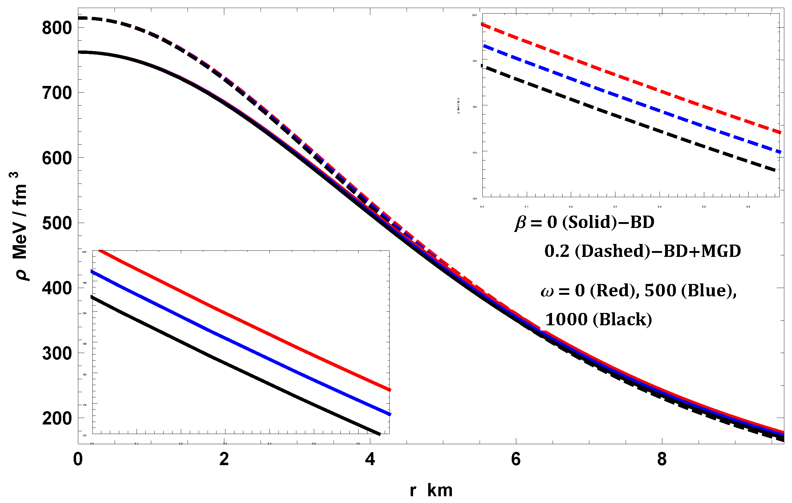
  • Figure 1, Figure 2 and Figure 3 show the variation of the matter density with respect to the radial coordinate for all chosen values of the parameters α , β and ω B D , respectively, by setting M = 1.97 M , R = 9.69 km, m ϕ = 0.001 , n = 0.01 , B = ( 0.0416 , 0.0415 ) / km, A = ( 0.38284 , 0.3857 ) and a = ( 0.0163 , 0.016 ) / km 2 . We can see from these plots that the matter density has its most extreme values at the center of the stellar structure and decreases monotonically towards the surface with an increasing radius, r. Additionally, it is positive everywhere inside the stellar configuration. Interestingly, the effect of the three parameters, α , β and ω B D , on the density energy, ρ , has been further demonstrated for both BD and BD+MGD scenarios, where any increase in α and β shifts the energy density, ρ , to higher equilibrium values throughout the stellar interior for all α [ 0.3 , 0.9 ] and β [ 0.0 , 1.0 ] , while any increase in ω B D shifts the energy density to lower equilibrium values throughout the stellar interior for all ω B D [ 0.0 , 1000 ] .
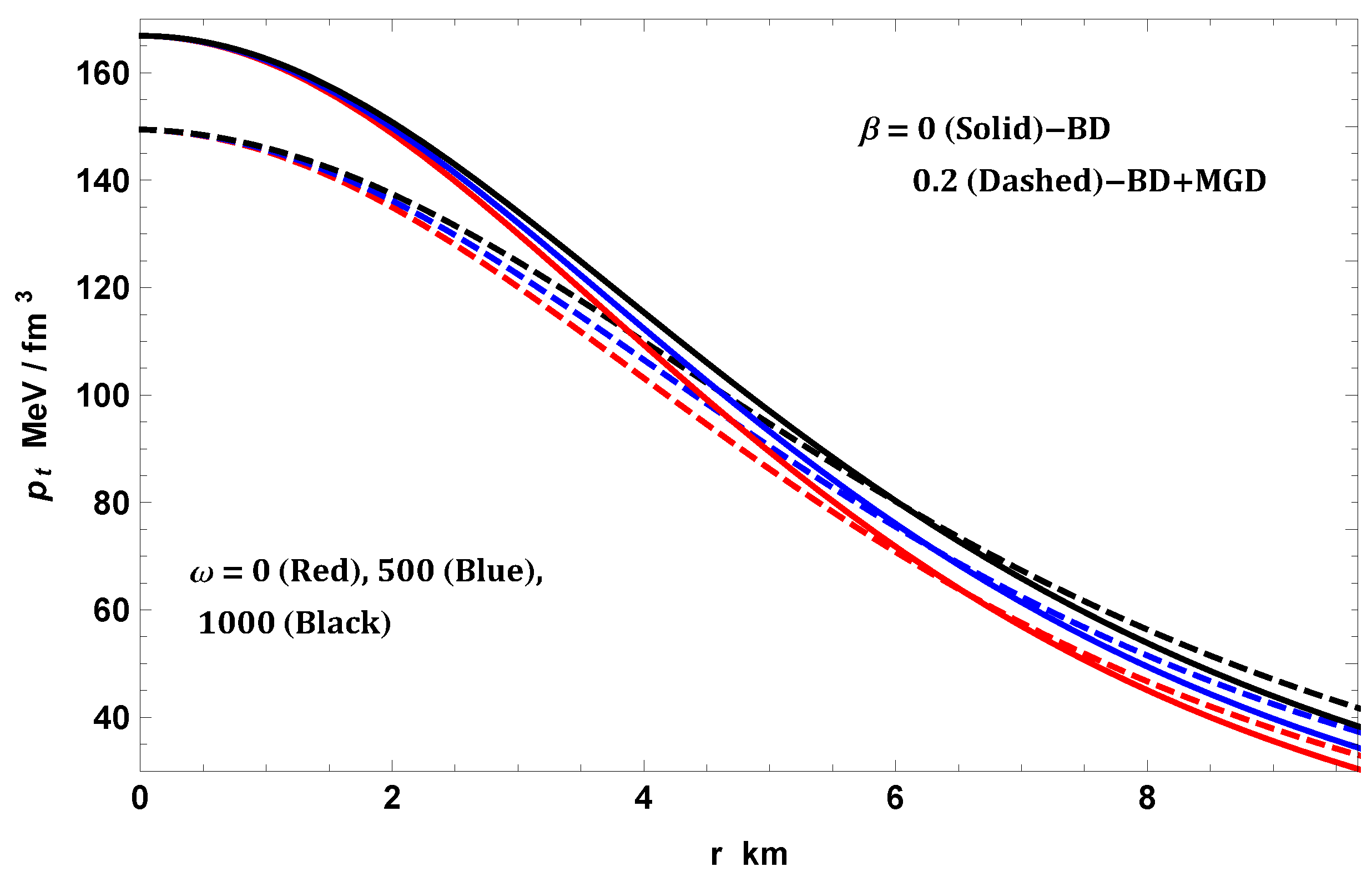
  • Figure 4, Figure 5, Figure 6, Figure 7 and Figure 8 display the variation of the radial and transverse pressures for the same parameters used in Figure 1, Figure 2 and Figure 3. From the five graphs, we can see that these physical amounts have their most extreme values at the core of the stellar object and are monotonic decreasing functions with increasing radial coordinates, r. Moreover, the radial pressure p r disappears at the surface of the stellar object, and the transverse p t one dominates at all points. It should be noted that the equilibrium values for p r and p t increase when α [ 0.3 , 0.9 ] increases from 0.3 to 0.9 , as illustrated in Figure 4 and Figure 7. In contrast, when we increase β [ 0.0 , 1.0 ] from 0.0 to 1.0 , the radially and tangentially outward pressures are reduced for both the BD and BD+MGD scenarios (see Figure 5). An emerging characteristic in Figure 6 and Figure 8 is that the parameter ω B D reduces the radially outward pressure and enhances the tangential surface stresses, as the parameter ω B D [ 0.0 , 1000 ] increases.
  • Figure 9, Figure 10 and Figure 11 exhibit the variation of anisotropy parameters for all the parameters taken into account in Figure 1, Figure 2 and Figure 3, whatever the interior of the stellar structure. Its comportment is positive at all points inside the stellar structure, disappearing at the core i.e., Δ = 0 , in impact at the core of the star p r = p t and has a monotonic increasing function with increasing radial coordinate, r. As we clarified above, Δ > 0 , which implies that p t > p r ; this presents that the system encounters a repulsive force (outwards). This last item counteracts the gravitational gradient progressing the stability and equilibrium state as well as one having more compact and massive stellar configurations. It is interesting evidence that the three parameters, α , β and ω B D , for both the BD and BD+MGD scenarios enhance the turbulence throughout the stellar interior, as Δ increases for α [ 0.3 , 0.9 ] , β [ 0.0 , 1.0 ] and ω B D [ 0.0 , 1000 ] , respectively (see Figure 9, Figure 10 and Figure 11 for more details).

7.2. Causality and Stability Condition

All through the adjustments introduced by the anisotropies source θ μ , ν in the stellar interior, we need to examine if the irritation presented by this new source provides to the stellar system a stable equilibrium. To do this, we employ Abreu’s criteria dependent on Herrera’s cracking approach [83]. Fundamentally, this criterion establishes the stability of compact stellar structures via the speeds of propagation related to the pressure waves in the principal directions of the spherical object i.e., in radial and transverse directions. Consequently, according to this criterion, the subliminal velocities corresponding to every direction are characterized by
v r 2 = d p r d ρ and v t 2 = d p t d ρ .
In order to obtain a genuinely allowable stellar system, the two velocities v r and v t should be limited by the velocity of light ( c = 1 in relativistic geometrized units). This reveals to us that the sound waves in the fluid do not spread at arbitrary velocities. This is known as the causality condition, which can be read as follows:
0 v r 1 and 0 v t 1 .
This causality condition is authoritative notwithstanding if the material substance of the stellar structure is isotropic or anisotropic and also has strong ramifications on the comportment of the matter distribution inside the stellar configuration. In this respect, from Figure 12, Figure 13 and Figure 14, we can observe that v r 2 and v r 2 fulfill the causality condition for all chosen values of the parameters α , β and ω B D , leading to a stable and viable stellar configuration under massive BD gravity via the MGD approach. It is intriguing to notice that v t is sensitive to changes in parameter strength, ω B D , in comparison to v r . The radial variation for both remains causal: v r [ 0.0 , 1.0 ] and v t [ 0.0 , 1.0 ] throughout the stellar interior.
Consequently, according to these three graphs, we can clearly see that our stellar system is fully stable under Abreu’s criteria based on Herrera’s cracking approach.

7.3. M R and M I Diagrams with Observational Data

We analyze the M R and M I curves generated from the solution under massive BD gravity and give a pedagogical clarification of the effects presented by gravitational decoupling by means of MGD with the choices made on parameters α and ω B D , in order to provide a more realistic scenario and reliable stellar system. In this connection, we bound the mentioned parameters by employing genuine observational data.
From Figure 15 and Figure 16, we give the total mass in Solar mass, i.e., M in M with the total radius R for the chosen specific values of parameters α and ω B D . In this respect, we have examined two cases. In the first case, we have made α vary according to values 0.3 , 0.5 , 0.7 , 0.9 , by fixing the BD-parameter ω B D to 5 as shown in Figure 15. In the second case, we varied ω B D as 0, 500, 1000, by fixing the parameter α to 0.5 as illustrated in Figure 16. In both cases, we also define the parameters: m ϕ = 0.001 , n = 0.01 , β = 0.2 , B = ( 0.0415 , 0.0416 / km, A = ( 0.3857 , 0.38284 ) and a = ( 0.016 , 0.0163 ) / km 2 . We sum up the new insights as follows:
  • Regarding the first case, Figure 15 highlights that, as the values of α increase, the maximal mass M and the corresponding radial coordinate R increase accordingly. Hence, this increase in the maximum mass on M R curves confirms the existence of gravitational decoupling (i.e., non-disappearing anisotropic term), which is expected. The most extreme mass in the M R curves is about 2.75 M , and in this manner, more massive compact stellar structures can be fitted. It also provides a direct correlation between the parameter, α , and the maximum mass, M, and its radius, R, where any increase in α shifts the stable compact stellar structure to a lower M at a lower confining radius for each α [ 0.3 , 0.9 ] . For instance, the highest maximum mass, M, is around 2.75 M , and its radius, R, is 9.35 km with α = 0.9 , while the lowest maximum mass, M, is 1.56 M , and its radius, R, is 5.40 km with α = 0.3 .
  • Regarding the second case, Figure 16 shows that the most extreme value of mass progressively decrements for the incrementing values of BD-parameter ω B D . In this regard, our anisotropic astrophysical stellar system becomes more massive and transforms into more compact stellar structures. We also demonstrate the impact of the parameter ω B D on the mass and its radius by considering values of ω B D , such that ω B D [ 0.0 , 1000 ] . We find that the maximum mass and its radius decrease as ω B D increases, for example, where the highest maximum mass, M, is 2.5512 M and its radius, R, is 8.76 km for ω B D = 0 ; the lowest maximum mass, M, is 2.484 M and its radius, R, is greater than 8.62 km for ω B D = 1000 .
Finally, for both cases, we have discovered a good adjustment for six compact stellar structures, viz., LMC X-4 (red), LMC X-4 (black), Her X-1 (blue), 4U 1820-30 (Orange), 4U 1608-52 (Cyan), SAX J1808.4-3658 (Purple) and many other compact stars that can be adjusted. On the other hand, it is clear how the two parameters α and ω B D presented by massive BD gravity incorporating the anisotropic comportment of the matter distribution has a great influence on many physical parameters of the stellar structure.
On the other hand, adopting the Bejger and Haensel concept [84], one can examine the moment of inertia I connecting to a static stellar solution, which could provide a precise tool for determining the stiffness of an equation of state (EoS). This concept is given by
I = 2 5 1 + ( M / R ) · k m M M R 2 .
In Figure 17 and Figure 18, we feature the variation of the maximum moment of inertia I with respect to the total mass M for the same values of parameters taken into consideration in M R curves, respectively. It is facile to see the effect of α and ω B D on I M curves from both figures for all the increasing value choices of the parameters α and ω B D . In this regard, we observe that the maximum moment of inertia I is always increasing from the null central value up to a specific mass value, and afterward decreases quickly. Therefore, we can conclude that the stiffness of the EoS is better through increasing the sensitivity of I M curves in both cases corresponding to the increase of the parameters α and ω B D . Moreover, our resulting I M curves are also equipped with observational data for the same well-known compact stellar structures fixed in M R curves, which are well fitted.

7.4. Mass–Central Density Relationship

To provide more investigations of the stability of the compact stellar system, we focus on the mass–density relation known as the static stability criterion, which is a significant thermodynamic amount. This static stability criterion was pointed out initially by Chandrashekhar [85] to describe the stability of a gaseous stellar structure according to radial perturbations. On the other hand, the development and simplification of this static stability criterion was envisaged by Harrison et al. [86] and Zeldovich and Novikov [87]. This Harrison–Zeldovich–Novikov static stability criterion infers that any solution describes static and stable stellar structure if the gravitational mass M is an increasing function of its central density ρ c i.e.,
M ( ρ c ) ρ c > 0 ,
or otherwise unstable if
M ( ρ c ) ρ c < 0 ,
under radial pulsation. From Figure 19 and Figure 20, it is easy to see that the gravitational mass is an increasing function with regard to central density, which fulfills the Harrison–Zeldovich–Novikov static stability criterion under radial pulsation. We can also observe that the stellar structures become more massive as ρ c is increased, and we found that the solution picks up its stability with an increase in all chosen values of different parameters, viz., α , β and ω B D in both scenarios BD in solid and BD+MGD in dashed as shown in Figure 19 and Figure 20.

8. Conclusions

The considered massive BD theory is one of the most extraordinary currently attainable alternative gravity theories that have huge deviations from the GRT on the one hand and are in concurrence with all the current observations on the other. Moreover, the massive BD theory is a well-posed theory which does not suffer from intrinsic problems and it is one of the best correct generalizations of GRT. This makes the solutions provided in this article and their stellar astrophysical implications very important.
In the present paper, we study the possibility of providing a new class of exact solutions for viable anisotropic stellar systems by means of massive BD gravity. In this regard, gravitational decoupling through the MGD approach in the arena of the embedding class-one space-time has effectively been employed to explore anisotropic solutions for matter sources. Our preliminary studies confirm that the decoupling of gravitational sources by MGD for compact stellar objects in massive BD gravity admitting the Karmarkar condition is a powerful mechanism to establish a more overall stellar solution of the modified Einstein field equations. For this purpose, we have constructed modified Einstein field equations given in (11)–(13), which disintegrate into two subsystems according to the MGD approach:
  • The first subsystem (standard Einstein’s system) corresponds to the field equations given in (24)–(26) with five unknown parameters, { Ψ , ξ , ρ , p r , p t } , and portrays the seed solution in BD gravity with respect to the stress-energy tensor T μ ν m .
  • The second subsystem (quasi-Einstein system) corresponds to the field equations expressed in (32)–(34) and examines the solution of a new θ -sector, which comprises mostly four unknown parameters, { h ( r ) , θ 0 0 , θ 1 1 , θ 2 2 } .
Hence, in order to solve the complete stellar system identified by these two subsystems, we have proposed two approaches, namely, the mimic requirement on density and pressure component for θ -sector, { θ 0 0 ( r ) = ρ ( r ) and θ 1 1 ( r ) = p r ( r ) } , respectively. For a detailed analysis for the massive stellar structure, we used the ansatz for Ψ relating to the notable, well-recognized and well-comported Finch–Skea model via the embedding class-one condition, as well as the deformation function indicated by h ( r ) via mimic requirement on the radial pressure component for anisotropic sector, viz., θ 1 1 ( r ) = p r ( r ) . It is worth mentioning that we have analyzed the stellar structures supported by an anisotropic matter distribution in the background of massive BD gravity via the MGD approach for several values of constant parameters depending on α , β and ω B D . The unknown parameters appearing in the anisotropic stellar system have been determined via matching the interior astrophysical stellar geometry for the system to the Schwarzschild line element that describes the vacuum in the exterior of the stellar structure. Moreover, for studying the physical validity of the accomplished solutions under massive BD gravity, we have analyzed various physical properties of the anisotropic astrophysical structure via the MGD approach, which can be summarized as follows:
  • We have observed in Figure 1, Figure 2, Figure 3, Figure 4, Figure 5, Figure 6, Figure 7 and Figure 8 that all the thermodynamic observables, in particular, matter density, radial and transverse pressures with respect to the radial coordinate r have maximum values at the center and show limited, positive and monotonic decreasing comportment gradually toward the minimum values at the boundary of the celestial bodies, while the radial pressure becomes zero at the surface, which affirms the physical suitability and agreeability of the envisaged solutions. From these plots, we affirm additionally that our celestial bodies are completely free from any physical or mathematical singularities for all various parametric values of α , β and ω B D .
  • The graphs corresponding to the comportment of anisotropy parameter Δ versus radial coordinate r are illustrated in Figure 9, Figure 10 and Figure 11. We see that the vanished anisotropy parameter Δ at the origin obtains positively defined increases to reach its maximum value at the surface of the stellar structure. Moreover, the fact that Δ > 0 i.e., p t > p r implies that the stellar system encounters a repulsive force that counteracts the gravitational gradient, progressing the stability and equilibrium state, as well as one that has more compact and massive celestial bodies.
  • The anisotropic stellar model is also consistent with the causality condition which is affirmed as the components of sound velocity lie within their prescribed bounds for all chosen values of the parameters α , β and ω B D , leading to a stable and viable compact stellar object under massive BD gravity via the MGD approach, as shown in Figure 12, Figure 13 and Figure 14.
  • Our investigation of the M R curves is very important for compact stellar objects and shows the maximal bound for the celestial bodies. In Figure 15 and Figure 16, we present the behavior of the total mass M (in Solar mass M ) with respect to the total radius R for the chosen specific values of parameters α and ω B D , by fixing β to 0.2 . In the current massive BD gravity model via the MGD approach, we find from Figure 15 that, due to α , as α increased, the maximum mass M increased with increasing radius R, which provides us with more massive compact stellar structures. On the other hand, as observed from Figure 16, due to ω B D , as ω B D increased, the maximum mass M decreased with increasing radius R, which provides us also a stellar system that is more compact and massive. On the other hand, we highlight the effect of α and ω B D , by fixing β to 0.2 , on the behavior of the maximum moment of inertia I against the total mass M, as illustrated in Figure 17 and Figure 18. From these graphs, we can conclude that the stiffness of the EoS is better through increasing the sensitivity of I M curves in both cases corresponding to the increase of the parameters, α and ω B D , which implies that the I m a x is always increasing from the zero up to a M m a x value, and thereafter decreases quickly. Finally, our generating M R and I M diagrams are well fitted with observational data, viz., LMC X-4, LMC X-4, Her X-1, 4U 1820-30, 4U 1608-52, SAX J1808.4-3658 and many other compact stellar structures that can be fitted. It is clear how both parameters α and ω B D presented by massive BD gravity via the MGD approach incorporating the anisotropic profile of the matter distribution has a great influence on many physical parameters of the compact stellar structures. Furthermore, the predicted radii for different compact objects are mentioned in Table 1 for different α and ω B D . It is observed that, for lower values of α , higher mass objects are ruled out. On the other hand, when α increases, compactness decreases, whereas compactness increases as ω B D increases.
  • It is well recognized that, for spherically symmetric static astrophysical systems, the Harrison–Zeldovich–Novikov static stability criterion plays a crucial role under radial pulsation, which must be satisfied to ensure stability. From Figure 19 and Figure 20, we observe that this static stability criterion is well satisfied under a radial perturbation, and we can also notice that the stellar structures become more massive as ρ c increases. Moreover, the stellar solution regains its stability with an increase in all chosen values of different parameters, viz., α , β and ω B D in both scenarios BD and BD+MGD.
Furthermore, it is mentioned that all the obtained results in this manuscript reduce to Einstein’s GR when φ = c o n s t a n t and ω B D .
Finally, we would like to mention here that all these new exact solutions for viable anisotropic stellar systems by means of massive BD gravity under gravitational decoupling through the MGD approach in the realm of the embedding class-one space-time are very much able to represent and describe the anisotropic compact celestial bodies.

Author Contributions

Conceptualization, S.K.M.; methodology, K.N.S.; software, K.N.S.; validation, M.K.J., K.N.S., S.K.M. and M.V.M.; formal analysis, K.N.S. and S.K.M.; investigation, M.K.J., A.E., S.K.M. and M.V.M.; data curation, K.N.S.; writing—original draft preparation, M.K.J., K.N.S., A.E. and S.K.M.; writing—review and editing, M.K.J., K.N.S., S.K.M. and M.V.M.; project administration, A.E. All authors have read and agreed to the published version of the manuscript.

Funding

E.A. thanks the National Research Foundation (NRF) of South Africa for the award of a postdoctoral fellowship.

Data Availability Statement

No data available or used.

Conflicts of Interest

The authors declare no conflict of interest.

Note

1
We denote m ( R ) = M = M ^ α R 2 h ( R ) , where M ^ is the total mass for the seed system.

References

  1. Schwarz, K. Static Solutions of Einstein’s Field Equations for Spheres of Fluid. Kl. Math. Phys. 1916, 24, 424. [Google Scholar]
  2. Tolman, R.C. Static Solutions of Einstein’s Field Equations for Spheres of Fluid. Phys. Rev. 1939, 55, 364. [Google Scholar] [CrossRef]
  3. Lemaitre, G. Annales de la Société scientifique de Bruxelles. Ann. Soc. Sci. Brux. 1933, A53, 51. [Google Scholar]
  4. Ruderman, R. Pulsars: Structure and Dynamics. Ann. Rev. Astron. Astrophys. 1972, 10, 427. [Google Scholar] [CrossRef]
  5. Bowers, R.L.; Liang, E.P.T. Anisotropic spheres in general relativity. Astrophys. J. 1974, 188, 657. [Google Scholar] [CrossRef]
  6. Herrera, L.; Santos, N.O. Local anisotropy in self-gravitating systems. Phys. Rep. 1997, 286, 53. [Google Scholar] [CrossRef]
  7. Harko, T.; Mak, M.K. Anisotropic relativistic stellar models. Ann. Phys. 2002, 11, 3. [Google Scholar] [CrossRef]
  8. Mak, M.K.; Harko, T. Anisotropic stars in general relativity. Proc. R Soc. Lond. Ser. A 2003, 459, 393. [Google Scholar] [CrossRef]
  9. Ivanov, B.V. Maximum bounds on the surface redshift of anisotropic stars. Phys. Rev. D 2002, 65, 104011. [Google Scholar] [CrossRef]
  10. Rahaman, F.; Ray, S.; Jafry, A.K.; Chakraborty, K. Singularity-free solutions for anisotropic charged fluids with Chaplygin equation of state. Phys. Rev. D 2010, 82, 104055. [Google Scholar] [CrossRef]
  11. Maurya, S.K.; Banerjee, A.; Hansraj, S. Role of pressure anisotropy on relativistic compact stars. Phys. Rev. D 2018, 97, 44022. [Google Scholar] [CrossRef]
  12. Maurya, S.K.; Banerjee, A.; Channuie, P. Relativistic compact stars with charged anisotropic matter. Chinese Phys. C 2018, 42, 55101. [Google Scholar] [CrossRef]
  13. Maurya, S.K.; Errehymy, A.; Deb, D.; Tello-Ortiz, F.; Daoud, M. Study of anisotropic strange stars in f(R,T) gravity: An embedding approach under the simplest linear functional of the matter-geometry coupling. Phys. Rev. D 2019, 100, 44014. [Google Scholar] [CrossRef]
  14. Maurya, S.K.; Banerjee, A.; Jasim, M.K.; Kumar, J.; Prasad, A.K.; Pradhan, A. Anisotropic compact stars in the Buchdahl model: A comprehensive study. Phys. Rev. D 2019, 99, 44029. [Google Scholar] [CrossRef]
  15. Tello-Ortiz, F.; Maurya, S.K.; Errehymy, A.; Singh, K.N.; Daoud, M. Anisotropic relativistic fluid spheres: An embedding class I approach. Eur. Phys. J. C 2019, 79, 885. [Google Scholar] [CrossRef]
  16. Deb, D.; Ketov, S.V.; Maurya, S.K.; Khlopov, M.; Moraes, P.H.R.S.; Ray, S. Exploring physical features of anisotropic strange stars beyond standard maximum mass limit in f(R, T) gravity. Mon. Not. R. Astron. Soc. 2019, 485, 5652. [Google Scholar] [CrossRef]
  17. Singh, K.N.; Maurya, S.K.; Errehymy, A.; Rahaman, F.; Daoud, M. Physical properties of class I compact star model for linear and Starobinsky-f(R,T) functions. Phys. Dark Univ. 2020, 30, 100620. [Google Scholar] [CrossRef]
  18. Rahaman, M.; Singh, K.N.; Errehymy, A.; Rahaman, F.; Daoud, M. Anisotropic Karmarkar stars in f(R, T)-gravity. Eur. Phys. J. C 2020, 80, 272. [Google Scholar] [CrossRef]
  19. Singh, K.N.; Errehymy, A.; Rahaman, F.; Daoud, M. Exploring physical properties of compact stars in f(R,T)-gravity: An embedding approach. Chinese Phys. C 2020, 44, 105106. [Google Scholar] [CrossRef]
  20. Ovalle, J. Searching exact solutions for compact stars in braneworld: A conjecture. Modern Phys. Lett. A 2008, 23, 3247. [Google Scholar] [CrossRef]
  21. Ovalle, J.; Linares, F. Nonminimal derivative coupling of a scalar field to gravity: Cosmological and black hole solutions. Phys. Rev. D 2013, 88, 104026. [Google Scholar] [CrossRef]
  22. Ovalle, J.; Casadio, R.; da Rocha, R.; Sotomayor, A. Anisotropic solutions by gravitational decoupling. Eur. Phys. J. C 2018, 78, 122. [Google Scholar] [CrossRef]
  23. Torres, V.; Contreras, E. Anisotropic neutron stars by gravitational decoupling. Eur. Phys. J. C 2019, 70, 829. [Google Scholar] [CrossRef]
  24. Ovalle, J. Decoupling gravitational sources in general relativity: From perfect to anisotropic fluids. Phys. Rev. D 2017, 95, 104019. [Google Scholar] [CrossRef]
  25. Casadio, R.; Nicolini, P.; da Rocha, R. Generalised uncertainty principle Hawking fermions from minimally geometric deformed black holes. Class. Quantum Grav. 2018, 35, 185001. [Google Scholar] [CrossRef]
  26. Hensh, R.; Stuchl’ik, Z. Anisotropic Tolman VII solution by gravitational decoupling. Eur. Phys. J. C 2019, 79, 834. [Google Scholar] [CrossRef]
  27. Sharif, M.; Saba, S. Gravitational decoupled anisotropic solutions in gravity. Eur. Phys. J. C 2018, 78, 921. [Google Scholar] [CrossRef]
  28. Estrada, M. A way of decoupling gravitational sources in pure Lovelock gravity. Eur. Phys. J. C 2019, 79, 918. [Google Scholar] [CrossRef]
  29. Maurya, S.K.; Tello-Ortiz, F. Charged anisotropic compact star in f (R, T) gravity: A minimal geometric deformation gravitational decoupling approach. Phys. Dark Univ. 2020, 27, 100442. [Google Scholar] [CrossRef]
  30. Maurya, S.K.; Errehymy, A.; Singh, K.N.; Tello-Ortiz, F.; Daoud, M. Gravitational decoupling minimal geometric deformation model in modified f (R, T) gravity theory. Phys. Dark Univ. 2020, 30, 100640. [Google Scholar] [CrossRef]
  31. Maurya, S.; Tello-Ortiz, F. Decoupling gravitational sources by MGD approach in Rastall gravity. Phys. Dark Univ. 2020, 29, 100577. [Google Scholar] [CrossRef]
  32. Cavalcanti, R.T.; Goncalves da Silva, A.; da Rocha, R. Strong deflection limit lensing effects in the minimal geometric deformation and Casadio–Fabbri–Mazzacurati solutions. Class. Quant. Gravit. 2016, 33, 215007. [Google Scholar] [CrossRef]
  33. Casadio, R.; da Rocha, R. Stability of the graviton Bose–Einstein condensate in the brane- world. Phys. Lett. B 2016, 763, 434. [Google Scholar] [CrossRef]
  34. da Rocha, R. Dark SU(N) glueball stars on fluid branes. Phys. Fire Up. D 2017, 95, 124017. [Google Scholar] [CrossRef]
  35. Casadio, R.; Ovalle, J.; da Rocha, R. The minimal geometric deformation approach extended. Class. Quant. Gravit. 2015, 32, 215020. [Google Scholar] [CrossRef]
  36. Ovalle, J. Decoupling gravitational sources in general relativity: The extended case. Phys. Lett. B 2019, 788, 213. [Google Scholar] [CrossRef]
  37. Sharif, M.; Ama-Tul-Mughani, Q. Anisotropic spherical solutions through extended gravitational decoupling approach. Ann. Phys. 2020, 415, 168122. [Google Scholar] [CrossRef]
  38. Sharif, M. Ama-Tul-Mughani, Q. Extended gravitational decoupled charged anisotropic solutions. Chin. J. Phys. 2020, 65, 207. [Google Scholar] [CrossRef]
  39. Ovalle, J.; Casadio, R.; da Rocha, R.; Sotomayor, A.; Stuchlik, Z. Black holes by gravitational decoupling. Eur. Phys. J. C 2018, 78, 960. [Google Scholar] [CrossRef]
  40. Contreras, E. Minimal Geometric Deformation: The inverse problem. Eur. Phys. J. C 2018, 78, 678. [Google Scholar] [CrossRef]
  41. Contreras, E.; Bargueno, P. Minimal geometric deformation in asymptotically (A-) dS space- times and the isotropic sector for a polytropic black hole. Eur. Phys. J. C 2018, 78, 985. [Google Scholar] [CrossRef]
  42. Rincon, A.; Gabbanelli, L.; Contreras, E.; Tello-Ortiz, F. Minimal geometric deformation in a Reissner–Nordström background. Eur. Phys. J. C 2019, 79, 873. [Google Scholar] [CrossRef]
  43. Zubair, M.; Azmat, H.; Amin, M. Charged anisotropic fluid sphere in comparison with its uncharged analogue through extended geometric deformation. Chin. J. Phys. 2022, 77, 898–914. [Google Scholar] [CrossRef]
  44. Maurya, S.K.; Singh, K.N.; Govender, M.; Hansraj, S. Gravitationally decoupled strange star model beyond the standard maximum mass limit in Einstein–Gauss–Bonnet gravity. Astrophys. J. 2022, 925, 208. [Google Scholar] [CrossRef]
  45. Briscese, F.; Elizalde, E.; Nojiri, S.; Odintsov, S.D. Phantom scalar dark energy as modified gravity: Understanding the origin of the Big Rip singularity. Phys. Lett. B 2007, 646, 105. [Google Scholar] [CrossRef]
  46. Nutku, Y. The post-Newtonian equations of hydrodynamics in the Brans–Dicke theory. Astrophys. J. 1969, 155, 999. [Google Scholar] [CrossRef]
  47. Kwon, O.J.; Kim Y., D.; Myung Y., S.; Cho B., H.; Park Y., J. Stability of the Schwarzschild black hole in Brans–Dicke theory. Phys. Rev. D 1986, 34, 333. [Google Scholar] [CrossRef]
  48. Shibata, M.; Nakao, K.; Nakamura, T. Scalar-type gravitational wave emission from gravitational collapse in Brans–Dicke theory: Detectability by a laser interferometer. Phys. Rev. D 1994, 50, 7304. [Google Scholar] [CrossRef]
  49. Harada, T.; Chiba, T.; Nakao, K.; Nakamura, T. Scalar gravitational wave from Oppenheimer- Snyder collapse in scalar-tensor theories of gravity. Phys. Rev. D 1997, 55, 2024. [Google Scholar] [CrossRef]
  50. Sharif, M.; Yousaf, Z. Stability of the charged spherical dissipative collapse in f(R) gravity. Mon. Not. R. Astron. Soc. 2013, 432, 264. [Google Scholar] [CrossRef]
  51. Dirac, P.A.M. A new basis for cosmology. Proc. R. Soc. A 1938, 165, 199. [Google Scholar] [CrossRef]
  52. Brans, C.H.; Dicke, R.H. principle and a relativistic theory of gravitation. Phys. Rev. 1961, 124, 925. [Google Scholar] [CrossRef]
  53. Faraoni, V. Cosmology in Scalar-Tensor Gravity; Springer: Berlin/Heidelberg, Germany, 2004. [Google Scholar]
  54. Bertotti, B.I.L.; Tortora, P. A test of general relativity using radio links with the Cassini spacecraft. Nature 2003, 425, 374. [Google Scholar] [CrossRef] [PubMed]
  55. Felice, A.D.; Mangano, G.; Serpico, P.; Trodden, M. Gauge-invariant formulation of second- order cosmological perturbations. Phys. Rev. D 2006, 74, 103005. [Google Scholar]
  56. Acquaviva, V.; Baccigalupi, C.; Leach, S.M.; Liddle, A.R.; Perrotta, F. Structure formation constraints on the Jordan-Brans–Dicke theory. Phys. Rev. D 2005, 71, 104025. [Google Scholar] [CrossRef]
  57. Liddle, A.R.; Mazumdar, A.; Barrow, J.D. Assisted inflation. Phys. Rev. D 1998, 58, 27302. [Google Scholar] [CrossRef]
  58. Chen, X.; Kamionkowski, M. Cosmic microwave background temperature and polarization anisotropy in Brans–Dicke cosmology. Phys. Rev. D 1999, 60, 104036. [Google Scholar] [CrossRef]
  59. Nagata, R.; Chiba, T.; Sugiyama, N. Chameleon cosmology. Phys. Rev. D 2004, 69, 83512. [Google Scholar] [CrossRef]
  60. Umiltà, C.; Ballardini, M.; Finelli, F.; Paoletti, D. CMB and BAO constraints for an induced gravity dark energy model with a quartic potential. J. Cosmol. Astropart. Phys. 2015, 17, 17. [Google Scholar] [CrossRef]
  61. Ballardini, M.; Finelli, F.; Umiltà, C.; Paoletti, D. Cosmological constraints on induced gravity dark energy models. J. Cosmol. Astropart. Phys. 2016, 1605, 67. [Google Scholar] [CrossRef]
  62. Rossi, M.; Ballardini, M.; Braglia, M.; Finelli, F.; Paoletti, D.; Starobinsky, A.A.; Umiltà, C. Cosmological constraints on post-Newtonian parameters in effectively massless scalar-tensor theories of gravity. Phys. Rev. D 2019, 100, 103524. [Google Scholar] [CrossRef]
  63. Koyama, K. Testing Brans–Dicke gravity with screening by scalar gravitational wave memory. Phys. Rev. D 2020, 102, 21502. [Google Scholar] [CrossRef]
  64. Sharif, M.; Majid, A. Anisotropic compact stars in self-interacting Brans–Dicke gravity. Astrophys. Space Sci. 2020, 365, 42. [Google Scholar] [CrossRef]
  65. Sharif, M.; Majid, A. Anisotropic strange stars through embedding technique in massive Brans–Dicke gravity. Eur. Phys. J. Plus 2020, 135, 558. [Google Scholar] [CrossRef]
  66. Sharif, M.; Majid, A. Extended gravitational decoupled solutions in self-interacting Brans–Dicke theory. Phys. Dark Univ. 2020, 30, 100610. [Google Scholar] [CrossRef]
  67. Sharif, M.; Majid, A. Isotropization and complexity of decoupled solutions in self- interacting Brans–Dicke gravity. Eur. Phys. J. Plus 2022, 137, 114. [Google Scholar] [CrossRef]
  68. Ramazanoglu, F.M.; Pretorius, F. Spontaneous scalarization with massive fields. Phys. Rev. D 2016, 93, 64005. [Google Scholar] [CrossRef]
  69. Yazadjiev, S.S.; Doneva, D.D.; Popchev, D. Slowly rotating neutron stars in scalar-tensor theories with a massive scalar field. Phys. Rev. D 2016, 93, 84038. [Google Scholar] [CrossRef]
  70. Doneva, D.D.; Yazadjiev, S.S. Rapidly rotating neutron stars with a massive scalar field—structure and universal relations. J. Cosmol. Astropart. Phys. 2016, 11, 19. [Google Scholar] [CrossRef]
  71. Staykov, K.V.; Popchev, D.; Doneva, D.D.; Yazadjiev, S.S. Static and slowly rotating neutron stars in scalar–tensor theory with self-interacting massive scalar field. Eur. Phys. J. C 2018, 78, 586. [Google Scholar] [CrossRef]
  72. Popchev, D.; Staykov, K.V.; Doneva, D.D.; Yazadjiev, S.S. Moment of inertia–mass universal relations for neutron stars in scalar- tensor theory with self-interacting massive scalar field. Eur. Phys. J. C 2019, 79, 178. [Google Scholar] [CrossRef]
  73. Bruckman, W.F.; Kazes, E. Properties of the solutions of cold ultradense configurations in the Brans–Dicke theory. Phys. Rev. D 1977, 16, 261. [Google Scholar] [CrossRef]
  74. Eisenhart, L.P. Riemannian Geometry; Princeton University Press: Princeton, NJ, USA, 1925; p. 97. [Google Scholar]
  75. Kasner, E. Finite Representation of the Solar Gravitational Field in Flat Space of Six Dimensions. Am. J. Math. 1921, 43, 130. [Google Scholar] [CrossRef]
  76. Gupta, Y.K.; Goel, M.P. Class two analogue of TY Thomas theorem and different types of embeddings of static spherically symmetric space-times. Gen. Rel. Grav. 1975, 6, 499. [Google Scholar] [CrossRef]
  77. Karmarkar, K.R. Gravitational metrics of spherical symmetry and class one. Proc. Indian Acad. Sci. 1948, 27, 56. [Google Scholar] [CrossRef]
  78. Pandey, S.N.; Sharma, S.P. Insufficiency of Karmarkar. condition. Gen. Relativ. Gravit. 1981, 14, 113. [Google Scholar] [CrossRef]
  79. O′Brien, S.; Synge, J.L. Jump Conditions at Discontinuities in General Relativity. Commun. Dublin Inst. Adv. Stud. A 1952, 9, 1–20. [Google Scholar]
  80. de Felice, F.; Yu, Y.; Fang, Z. Relativistic charged spheres. Mon. Not. R. Astron. Soc. 1995, 277, L17. [Google Scholar]
  81. Morales, E.; Tello-Ortiz, F. Compact anisotropic models in general relativity by gravitational decoupling. Eur. Phys. J. C 2018, 78, 841. [Google Scholar] [CrossRef]
  82. Morales, E.; Tello-Ortiz, F. Charged anisotropic compact objects by gravitational decoupling. Eur. Phys. J. C 2018, 78, 618. [Google Scholar] [CrossRef]
  83. Abreu, H.; Hernandez, H.; Nunez, L.A. Sound speeds, cracking and the stability of self- gravitating anisotropic compact objects. Class. Quant. Grav. 2007, 24, 4631. [Google Scholar] [CrossRef]
  84. Bejger, M.; Haensel, P. Moments of inertia for neutron and strange stars: Limits derived for the Crab pulsar. A. & A. 2002, 396, 917. [Google Scholar]
  85. Chandrasekhar, S. Dynamical instability of gaseous masses approaching the Schwarzschild limit in general relativity. Phys. Rev. Lett. 1964, 12, 114. [Google Scholar] [CrossRef]
  86. Harrison, B.K.; Thorne, K.S.; Wakano, M.; Wheeler, J.A. Gravitational Theory and Gravitational Collapse; University of Chicago Press: Chicago, IL, USA, 1966. [Google Scholar]
  87. Zeldovich, Y.B.; Novikov, I.D. Relativistic Astrophysics: Stars and Relativity; University of Chicago Press: Chicago, IL, USA, 1971. [Google Scholar]
  88. Abubekerov, M.K.; Antokhina, E.A.; Cherepashchuk, A.M.; Shimanskii, V.V. The mass of the compact object in the X-ray binary her X-1/HZ her. Astron. Rep. 2008, 52, 379. [Google Scholar] [CrossRef]
  89. Elebert, P.; Reynolds, M.T.; Callanan, P.J.; Hurley, D.J.; Ramsay, G.; Lewis, F.; Russell, D.M.; Nord, B.; Kane, S.R.; DePoy, D.L.; et al. Optical spectroscopy and photometry of SAX J1808.4-3658 in outburst. Mon. Not. R. Astron. Soc. 2009, 395, 884. [Google Scholar] [CrossRef]
  90. Rawls, M.L.; Orosz, J.A.; McClintock, J.E.; Torres, M.A.P.; Bailyn, C.D.; Buxton, M.M. Refined Neutron Star Mass Determinations for Six Eclipsing X-Ray Pulsar Binaries. ApJ 2011, 730, 25. [Google Scholar] [CrossRef]
  91. Güver, T.; Wroblewski, P.; Camarota, L.; Ózel, F. The Distance, Mass, and Radius of the Neutron Star in 4U 1608-52. Astrophys. J. 2010, 712, 964. [Google Scholar] [CrossRef]
  92. Güver, T.; Wroblewski, P.; Camarota, L.; Ózel, F. The Mass and Radius of the Neutron Star in 4U 1820-30. Astrophys. J. 2010, 719, 1807. [Google Scholar] [CrossRef]
Figure 1. Variation of matter density against r for M = 1.97 M , R = 9.69 km , ω B D = 5 , m ϕ = 0.001 , n = 0.01 , β = ( 0 , 0.2 ) , B = ( 0.0416 , 0.0415 ) / km , A = ( 0.38284 , 0.3857 ) and a = ( 0.0163 , 0.016 ) / km 2 .
Universe 09 00208 g001
Figure 2. Variation of matter density against r for M = 1.97 M , R = 9.69 km , ω B D = 5 , m ϕ = 0.001 , B = 0.0415 / km , n = 0.01 , α = 0.15 , A = 0.3857 and a = 0.016 / km 2 .
Universe 09 00208 g002
Figure 3. Variation of matter density against r for M = 1.97 M , R = 9.69 km , α = 0.5 , m ϕ = 0.001 , n = 0.01 , β = ( 0 , 0.2 ) , B = 0.0416 / km , A = 0.38284 and a = 0.0163 / km 2 .
Universe 09 00208 g003
Figure 4. Variation of radial pressure against r for M = 1.97 M , R = 9.69 km , ω B D = 5 , m ϕ = 0.001 , n = 0.01 , β = ( 0 , 0.2 ) , B = ( 0.0416 , 0.0415 ) / km , A = ( 0.38284 , 0.3857 ) and a = ( 0.0163 , 0.016 ) / km 2 .
Universe 09 00208 g004
Figure 5. Variation of pressures against r for M = 1.97 M , R = 9.69 km , ω B D = 5 , m ϕ = 0.001 , B = 0.0415 / km, n = 0.01 , α = 0.15 , A = 0.3857 and a = 0.016 / km 2 .
Universe 09 00208 g005
Figure 6. Variation of radial pressure against r for M = 1.97 M , R = 9.69 km , α = 0.5 , m ϕ = 0.001 , n = 0.01 , β = ( 0 , 0.2 ) , B = 0.0416 / km , A = 0.38284 and a = 0.0163 / km 2 .
Universe 09 00208 g006
Figure 7. Variation of transverse pressure against r for M = 1.97 M , R = 9.69 km , ω B D = 5 , m ϕ = 0.001 , n = 0.01 , β = ( 0 , 0.2 ) , B = ( 0.0416 , 0.0415 ) / km , A = ( 0.38284 , 0.3857 ) and a = ( 0.0163 , 0.016 ) / km 2 .
Universe 09 00208 g007
Figure 8. Variation of transverse pressure against r for M = 1.97 M , R = 9.69 km , α = 0.5 , m ϕ = 0.001 , n = 0.01 , β = ( 0 , 0.2 ) , B = 0.0416 / km , A = 0.38284 and a = 0.0163 / km 2 .
Universe 09 00208 g008
Figure 9. Variation of anisotropy against r for M = 1.97 M , R = 9.69 km , ω B D = 5 , m ϕ = 0.001 , n = 0.01 , β = ( 0 , 0.2 ) , B = ( 0.0416 , 0.0415 ) / km , A = ( 0.38284 , 0.3857 ) and a = ( 0.0163 , 0.016 ) / km 2 .
Universe 09 00208 g009
Figure 10. Variation of anisotropy against r for M = 1.97 M , R = 9.69 km , ω B D = 5 , m ϕ = 0.001 , B = 0.0415 / km , n = 0.01 , α = 0.15 , A = 0.3857 and a = 0.016 / km 2 .
Universe 09 00208 g010
Figure 11. Variation of anisotropy against r for M = 1.97 M , R = 9.69 km , α = 0.5 , m ϕ = 0.001 , n = 0.01 , β = ( 0 , 0.2 ) , B = 0.0416 / km , A = 0.38284 and a = 0.0163 / km 2 .
Universe 09 00208 g011
Figure 12. Variation of sound velocity against r for M = 1.97 M , R = 9.69 km , ω B D = 5 , m ϕ = 0.001 , n = 0.01 , β = ( 0 , 0.2 ) , B = ( 0.0416 , 0.0415 ) / km , A = ( 0.38284 , 0.3857 ) and a = ( 0.0163 , 0.016 ) / km 2 .
Universe 09 00208 g012
Figure 13. Variation of sound velocity against r for M = 1.97 M , R = 9.69 km , ω B D = 5 , m ϕ = 0.001 , B = 0.0415 / km , n = 0.01 , α = 0.15 , A = 0.3857 and a = 0.016 / km 2 .
Universe 09 00208 g013
Figure 14. Variation of sound velocity against r for M = 1.97 M , R = 9.69 km , α = 0.5 , m ϕ = 0.001 , n = 0.01 , β = ( 0 , 0.2 ) , B = 0.0416 / km , A = 0.38284 and a = 0.0163 / km 2 .
Universe 09 00208 g014
Figure 15. M R curve for ω B D = 5 , m ϕ = 0.001 , n = 0.01 , β = 0.2 , B = ( 0.0415 ) / km , A = 0.3857 and a = 0.016 / km 2 .
Universe 09 00208 g015
Figure 16. M R curve for α = 0.5 , m ϕ = 0.001 , n = 0.01 , β = 0.2 , B = 0.0416 / km , A = 0.38284 and a = 0.0163 / km 2 .
Universe 09 00208 g016
Figure 17. M I curve for ω B D = 5 , m ϕ = 0.001 , n = 0.01 , β = 0.2 , B = ( 0.0415 ) / km , A = 0.3857 and a = 0.016 / km 2 .
Universe 09 00208 g017
Figure 18. M I curve for k m , α = 0.5 , m ϕ = 0.001 , n = 0.01 , β = 0.2 , B = 0.0416 / km , A = 0.38284 and a = 0.0163 / km 2 .
Universe 09 00208 g018
Figure 19. m ( ρ c ) ρ c curves for α = 0.5 , m ϕ = 0.001 , n = 0.01 , β = ( 0 , 0.2 ) , B = 0.0416 / km and A = 0.38284 .
Universe 09 00208 g019
Figure 20. m ( ρ c ) ρ c curves for ω B D = 5 , m ϕ = 0.001 , B = 0.0415 / km , n = 0.01 , α = 0.7 and A = 0.3857 .
Universe 09 00208 g020
Table 1. Physical parameters of the observed compact stars for constants used in Figure 15 and Figure 16.
Predicted Radii (km)
Strange StarsObserved Mass α ω BD
( M ) 0.30.50.70.905001000
Her X-10.85 ± 0.15 [88]5.586.837.768.528.118.0968.066
SAX J1808.4-36580.9 ± 0.3 [89]5.636.917.868.648.248.218.18
SMC X-11.04 ± 0.09 [90]5.827.398.509.418.958.898.83
LMC X-41.29 ± 0.05 [90]5.757.128.108.968.548.488.45
4U 1820-301.58 ± 0.06 [91]-7.518.779.779.279.199.11
4U 1608-521.74 ± 0.14 [92]-7.498.569.928.278.218.175
Disclaimer/Publisher’s Note: The statements, opinions and data contained in all publications are solely those of the individual author(s) and contributor(s) and not of MDPI and/or the editor(s). MDPI and/or the editor(s) disclaim responsibility for any injury to people or property resulting from any ideas, methods, instructions or products referred to in the content.

