
sunRunner1D: A Tool for Exploring ICME Evolution through the Inner Heliosphere

Abstract
:1. Introduction
2. Materials and Methods
2.1. Events
2.2. Model
2.3. Data
3. Results
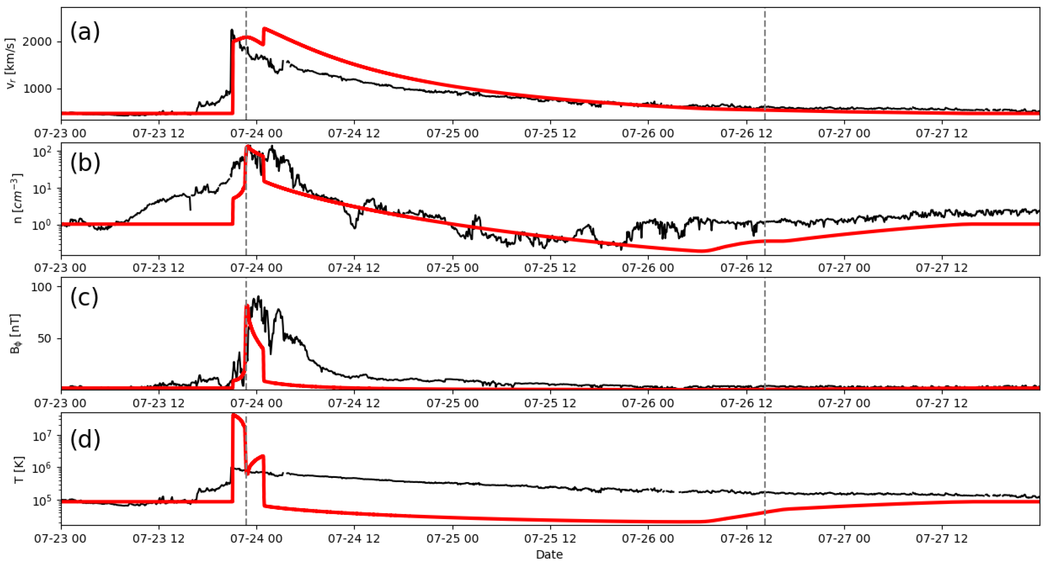
3.1. Event 1
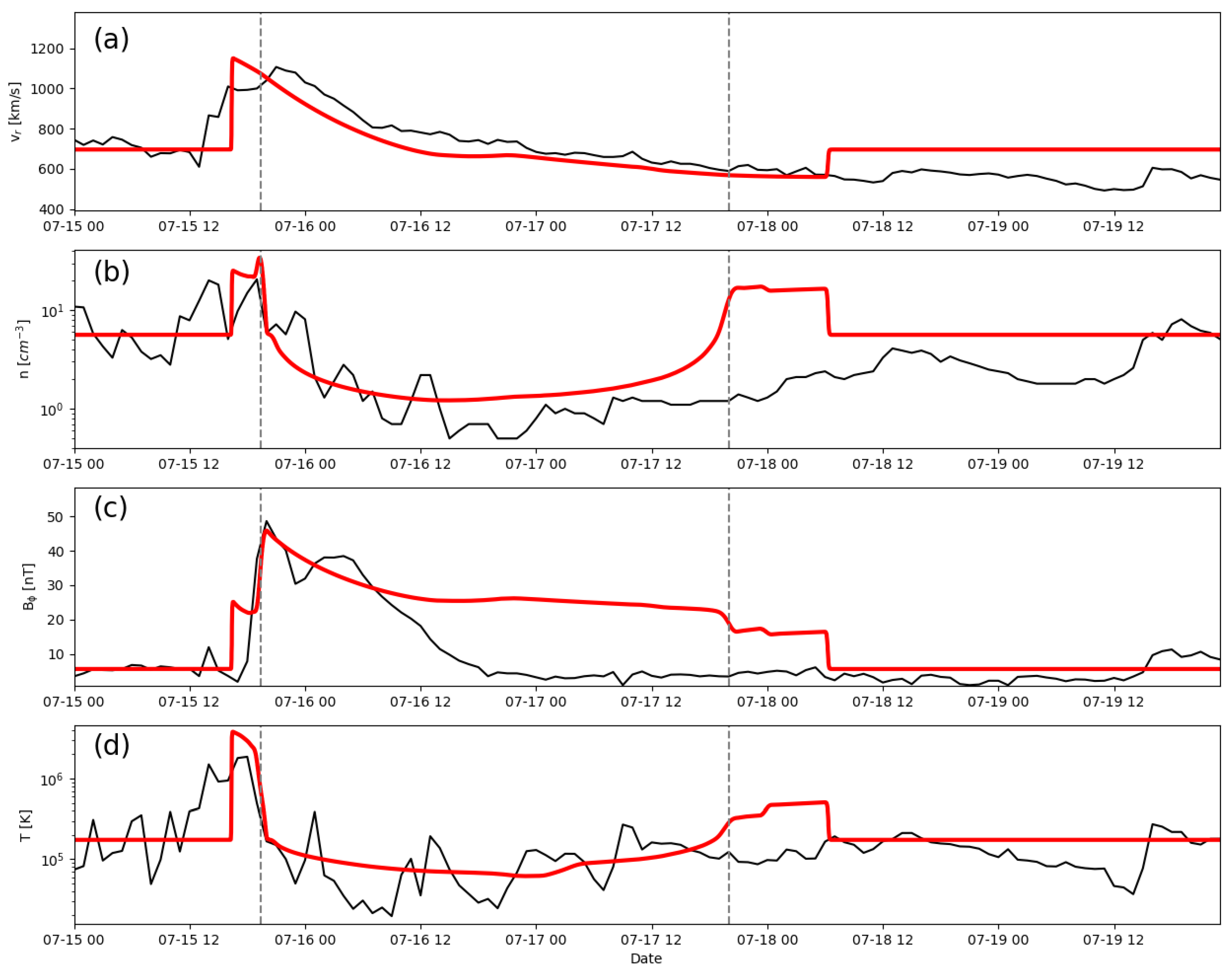
3.2. Event 2
3.3. Event 3
3.4. Event 4
4. Discussion
Author Contributions
Funding
Data Availability Statement
Acknowledgments
Conflicts of Interest
References
- Gosling, J.T. Coronal mass ejections and magnetic flux ropes in interplanetary space. IN Phys. Magn. Flux Ropes 1990, 58, 343. [Google Scholar]
- Hundhausen, A.J. Some macroscopic properties of shock waves in the heliosphere. IN Collisionless Shock. Heliosphere A Tutor. Rev. 1985, 34, 37. [Google Scholar]
- Dryer, M.; Smith, Z.; Fry, C.; Sun, W.; Deehr, C.; Akasofu, S.I. Real-time shock arrival predictions during the “Halloween 2003 epoch”. Space Weather 2004, 2, S09001. [Google Scholar] [CrossRef]
- Manchester, W.B.; Gombosi, T.I.; Roussev, I.; De Zeeuw, D.L.; Sokolov, I.V.; Powell, K.G.; Tóth, G.; Opher, M. Three-dimensional MHD simulation of a flux rope driven CME. J. Geophys. Res. 2004, 109, 1102. [Google Scholar] [CrossRef]
- Riley, P.; Lionello, R.; Mikić, Z.; Linker, J. Using Global Simulations to Relate the Three-Part Structure of Coronal Mass Ejections to In Situ Signatures. Astrophys. J. 2008, 672, 1221–1227. [Google Scholar] [CrossRef]
- Odstrcil, D. Numerical Simulation of Interplanetary Disturbances. In Astronomical Society of the Pacific Conference Series; Pogorelov, N.V., Audit, E., Colella, P., Zank, G.P., Eds.; Astronomical Society of the Pacific: San Francisco, CA, USA, 2009; Volume 406, p. 141. [Google Scholar]
- Török, T.; Downs, C.; Linker, J.A.; Lionello, R.; Titov, V.S.; Mikić, Z.; Riley, P.; Caplan, R.M.; Wijaya, J. Sun-to-Earth MHD Simulation of the 2000 July 14 “Bastille Day” Eruption. Astrophys. J. 2018, 856, 75. [Google Scholar] [CrossRef]
- Owens, M.; Lang, M.; Barnard, L.; Riley, P.; Ben-Nun, M.; Scott, C.J.; Lockwood, M.; Reiss, M.A.; Arge, C.N.; Gonzi, S. A computationally efficient, time-dependent model of the solar wind for use as a surrogate to three-dimensional numerical magnetohydrodynamic simulations. Sol. Phys. 2020, 295, 1–17. [Google Scholar] [CrossRef]
- Riley, P.; Linker, J.A.; Lionello, R.; Mikić, Z.; Odstrcil, D.; Hidalgo, M.A.; Cid, C.; Hu, Q.; Lepping, R.P.; Lynch, B.J.; et al. Fitting flux ropes to a global MHD solution: A comparison of techniques. J. Atmos.-Sol.-Terr. Phys. 2004, 66, 1321–1331. [Google Scholar] [CrossRef]
- Pizzo, V.; Koning, C.; Cash, M.; Millward, G.; Biesecker, D.; Puga, L.; Codrescu, M.; Odstrcil, D. Theoretical basis for operational ensemble forecasting of coronal mass ejections. Space Weather 2015, 13, 676–697. [Google Scholar] [CrossRef]
- Mignone, A.; Bodo, G.; Massaglia, S.; Matsakos, T.; Tesileanu, O.; Zanni, C.; Ferrari, A. PLUTO: A numerical code for computational astrophysics. Astrophys. J. Suppl. Ser. 2007, 170, 228. [Google Scholar] [CrossRef]
- Baker, D.; Li, X.; Pulkkinen, A.; Ngwira, C.; Mays, M.; Galvin, A.; Simunac, K. A major solar eruptive event in July 2012: Defining extreme space weather scenarios. Space Weather 2013, 11, 585–591. [Google Scholar] [CrossRef]
- Riley, P.; Caplan, R.M.; Giacalone, J.; Lario, D.; Liu, Y. Properties of the Fast Forward Shock Driven by the July 23 2012 Extreme Coronal Mass Ejection. Astrophys. J. 2016, 819, 57. [Google Scholar] [CrossRef] [Green Version]
- Gosling, J.T.; Riley, P.; McComas, D.J.; Pizzo, V.J. Overexpanding coronal mass ejections at high heliographic latitudes—Observations and simulations. J. Geophys. Res. 1998, 103, 1941. [Google Scholar] [CrossRef]
- Gosling, J.T.; Bame, S.J.; McComas, D.J.; Phillips, J.L.; Scime, E.E.; Pizzo, V.J.; Goldstein, B.E.; Balogh, A. A forward-reverse shock pair in the solar wind driven by over-expanison of a coronal mass ejection: Ulysses observations. Geophys. Res. Lett. 1994, 21, 237–240. [Google Scholar] [CrossRef]
- Tokumaru, M.; Kojima, M.; Fujiki, K.; Yamashita, M.; Yokobe, A. Toroidal-shaped interplanetary disturbance associated with the halo coronal mass ejection event on 14 July 2000. J. Geophys. Res. Space Phys. 2003, 108, 1220. [Google Scholar] [CrossRef]
- Nieves-Chinchilla, T.; Szabo, A.; Korreck, K.E.; Alzate, N.; Balmaceda, L.A.; Lavraud, B.; Paulson, K.; Narock, A.A.; Wallace, S.; Jian, L.K.; et al. Analysis of the internal structure of the streamer blowout observed by the parker solar probe during the first solar encounter. Astrophys. J. Suppl. Ser. 2020, 246, 63. [Google Scholar] [CrossRef]
- Korreck, K.E.; Szabo, A.; Chinchilla, T.N.; Lavraud, B.; Luhmann, J.; Niembro, T.; Higginson, A.; Alzate, N.; Wallace, S.; Paulson, K.; et al. Source and propagation of a streamer blowout coronal mass ejection observed by the Parker Solar Probe. Astrophys. J. Suppl. Ser. 2020, 246, 69. [Google Scholar] [CrossRef]
- Wold, A.M.; Mays, M.L.; Taktakishvili, A.; Jian, L.K.; Odstrcil, D.; MacNeice, P. Verification of real-time WSA− ENLIL+ Cone simulations of CME arrival-time at the CCMC from 2010 to 2016. J. Space Weather Space Clim. 2018, 8, A17. [Google Scholar] [CrossRef]
- Pomoell, J.; Poedts, S. EUHFORIA: European heliospheric forecasting information asset. J. Space Weather Space Clim. 2018, 8, A35. [Google Scholar] [CrossRef]
- Riley, P.; Lionello, R.; Caplan, R.M.; Downs, C.; Linker, J.A.; Badman, S.T.; Stevens, M.L. Using Parker Solar Probe observations during the first four perihelia to constrain global magnetohydrodynamic models. Astron. Astrophys. 2021, 650, A19. [Google Scholar] [CrossRef]
- King, J.H.; Papitashvili, N.E. Solar wind spatial scales in and comparisons of hourly Wind and ACE plasma and magnetic field data. J. Geophys. Res. 2005, 110, 2104. [Google Scholar] [CrossRef]
- Liu, Y.D.; Luhmann, J.G.; Kajdič, P.; Kilpua, E.K.; Lugaz, N.; Nitta, N.V.; Möstl, C.; Lavraud, B.; Bale, S.D.; Farrugia, C.J.; et al. Observations of an extreme storm in interplanetary space caused by successive coronal mass ejections. Nat. Commun. 2014, 5, 3481. [Google Scholar] [CrossRef] [PubMed] [Green Version]
- Temmer, M.; Nitta, N. Interplanetary Propagation Behavior of the Fast Coronal Mass Ejection on 23 July 2012. Sol. Phys. 2015, 290, 919–932. [Google Scholar] [CrossRef]
- Russell, C.T.; Mewaldt, R.A.; Luhmann, J.G.; Mason, G.M.; von Rosenvinge, T.T.; Cohen, C.M.S.; Leske, R.A.; Gomez-Herrero, R.; Klassen, A.; Galvin, A.B.; et al. The Very Unusual Interplanetary Coronal Mass Ejection of 2012 July 23: A Blast Wave Mediated by Solar Energetic Particles. Astrophys. J. 2013, 770, 38. [Google Scholar] [CrossRef]
- Ngwira, C.M.; Pulkkinen, A.; Leila Mays, M.; Kuznetsova, M.M.; Galvin, A.; Simunac, K.; Baker, D.N.; Li, X.; Zheng, Y.; Glocer, A. Simulation of the 23 July 2012 extreme space weather event: What if this extremely rare CME was Earth directed? Space Weather 2013, 11, 671–679. [Google Scholar] [CrossRef]
- Liu, Y.C.M.; Galvin, A.B.; Popecki, M.A.; Simunac, K.D.C.; Kistler, L.; Farrugia, C.; Lee, M.A.; Klecker, B.; Bochsler, P.; Luhmann, J.L.; et al. Proton enhancement and decreased O6+/H at the heliospheric current sheet: Implications for the origin of slow solar wind. Twelfth Int. Sol. Wind Conf. AIP Conf. Proc. 2010, 1216, 363. [Google Scholar] [CrossRef]
- Desai, R.T.; Zhang, H.; Davies, E.E.; Stawarz, J.E.; Mico-Gomez, J.; Iváñez-Ballesteros, P. Three-dimensional simulations of solar wind preconditioning and the 23 July 2012 interplanetary coronal mass ejection. Sol. Phys. 2020, 295, 1–14. [Google Scholar] [CrossRef]
- Gosling, J.T.; McComas, D.J.; Phillips, J.L.; Weiss, L.A.; Pizzo, V.J.; Goldstein, B.E.; Forsyth, R.J. A new class of forward-reverse shock pairs In the solar wind. Geophys. Res. Lett. 1994, 21, 2271. [Google Scholar] [CrossRef]
- Bothmer, V.; Desai, M.I.; Marsden, R.G.; Sanderson, T.R.; Trattner, K.J.; Wenzel, K.P.; Gosling, J.T.; Balogh, A.; Forsyth, R.J.; Goldstein, B.E. Ulysses observations of open and closed magnetic field lines within a coronal mass ejection. Astron. Astrophys. 1996, 316, 493–498. [Google Scholar]
- Smith, E.J.; Jokipii, J.R.; Kóta, J.; Lepping, R.P.; Szabo, A. Evidence of a North–South Asymmetry in the Heliosphere Associated with a Southward Displacement of the Heliospheric Current Sheet. Astrophys. J. 2000, 533, 1084–1089. [Google Scholar] [CrossRef]
- Pizzo, V.J. A three-dimensional model of corotating streams in the solar wind. III—Magnetohydrodynamic streams. J. Geophys. Res. 1982, 87, 4374. [Google Scholar] [CrossRef]
- Gosling, J.; Pizzo, V. Formation and evolution of corotating interaction regions and their three dimensional structure. Corotating Interact. Reg. 1999, 89, 21–52. [Google Scholar]
- Falconer, D.A.; Moore, R.L.; Gary, G.A. Correlation of the Coronal Mass Ejection Productivity of Solar Active Regions with Measures of Their Global Nonpotentiality from Vector Magnetograms: Baseline Results. Astrophys. J. 2002, 569, 1016–1025. [Google Scholar] [CrossRef]
- Linker, J.; Downs, C.; Caplan, R.M.; Riley, P.; Titov, V.S.; Lionello, R.; Torok, T.; Reyes, A. Prediction of Coronal Structure for the July 2, 2019 Total Solar Eclipse: Comparison with Observations. Am. Geophys. Union Fall Meet. 2019, 2019, SH13A-04. [Google Scholar]
- Riley, P.; Mays, M.L.; Andries, J.; Amerstorfer, T.; Biesecker, D.; Delouille, V.; Dumbović, M.; Feng, X.; Henley, E.; Linker, J.A.; et al. Forecasting the Arrival Time of Coronal Mass Ejections: Analysis of the CCMC CME Scoreboard. Space Weather 2018, 16, 1245–1260. [Google Scholar] [CrossRef] [Green Version]


| ICME No. | Date | Spacecraft | Type of CME | References |
|---|---|---|---|---|
| 1 | 23 July 2012 | STEREO-A | Extreme (fast) | Baker et al. [12], Riley et al. [13] |
| 2 | 21 April 1994 | Ulysses | Overexpanding | Gosling et al. [14], Gosling et al. [15] |
| 3 | 14 July 2000 | ACE/WIND | Multiple (3) interacting | Török et al. [7], Tokumaru et al. [16] |
| 4 | 12 November 2018 | PSP | Streamer-blowout (slow) | Nieves-Chinchilla et al. [17], Korreck et al. [18] |
| Event | (km s−1) | (km s−1) | (nT) | (nT) | (cm−3) | (cm−3) | (K) | (h) |
|---|---|---|---|---|---|---|---|---|
| 1 | 410 | 1977 | 15.6 | 126.6 | 69 | 1870 | 7.15 × 10⁵ | 19.6 |
| 2 | 462 | 0.0 | 10.4 | 55.4 | 226 | 1208 | 5.0 × 10⁶ | 7.0 |
| 3 | 616 | 238 | 48.7 | 976 | 377 | 0.0 | 1.43 × 10⁶ | 17.7 |
| 4 | 250 | 0.0 | 59.8 | 1195 | 1276 | 1914 | 9.2 × 10⁵ | 3.0 |
Publisher’s Note: MDPI stays neutral with regard to jurisdictional claims in published maps and institutional affiliations. |
© 2022 by the authors. Licensee MDPI, Basel, Switzerland. This article is an open access article distributed under the terms and conditions of the Creative Commons Attribution (CC BY) license (https://creativecommons.org/licenses/by/4.0/).
Share and Cite
Riley, P.; Ben-Nun, M. sunRunner1D: A Tool for Exploring ICME Evolution through the Inner Heliosphere. Universe 2022, 8, 447. https://doi.org/10.3390/universe8090447
Riley P, Ben-Nun M. sunRunner1D: A Tool for Exploring ICME Evolution through the Inner Heliosphere. Universe. 2022; 8(9):447. https://doi.org/10.3390/universe8090447
Chicago/Turabian StyleRiley, Pete, and Michal Ben-Nun. 2022. "sunRunner1D: A Tool for Exploring ICME Evolution through the Inner Heliosphere" Universe 8, no. 9: 447. https://doi.org/10.3390/universe8090447