


Multiple SSO Space Debris Flyby Trajectory Design Based on Cislunar Orbit

Abstract
:1. Introduction
2. Problem Statement and Equations of Motion
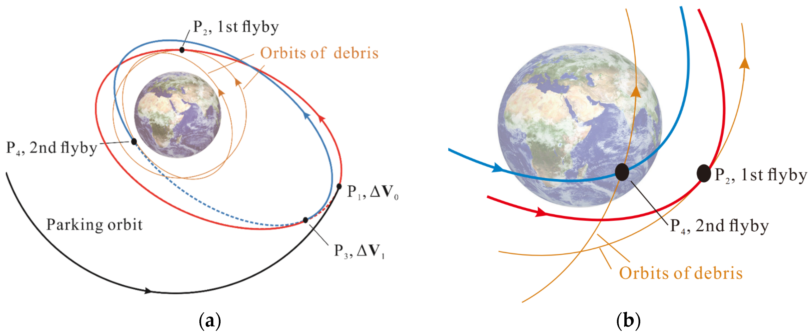
2.1. General Scenario
2.2. Parking Orbit
- (1)
- The parking orbit should be long-term stable.
- (2)
- A small velocity increment is demanded for the spacecraft to transfer from the parking orbit to flyby multiple SSO targets.
- (3)
- The apogee of the parking orbit should be large so that it would be easier for the spacecraft to adjust the orbital inclination, which is more favorable for multiple-object near-coplanar flyby missions.
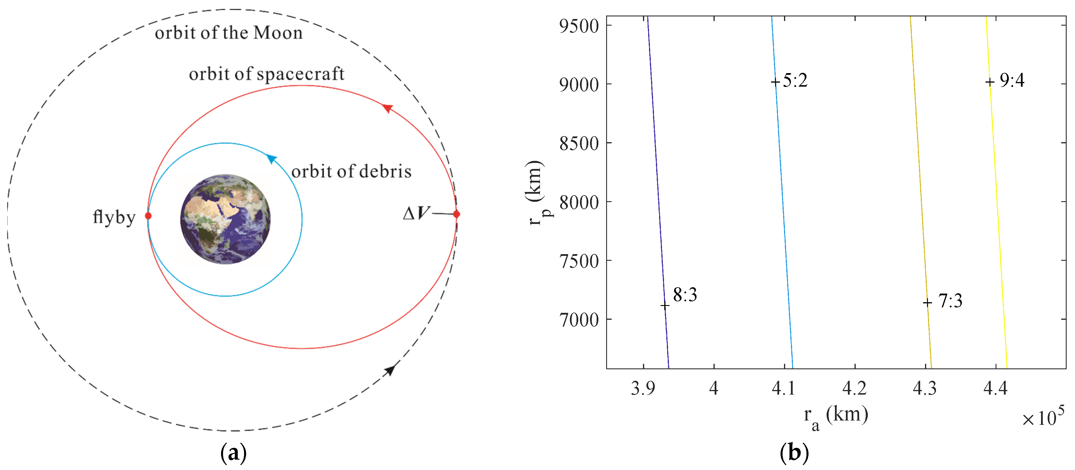
2.3. Flyby Mission Description
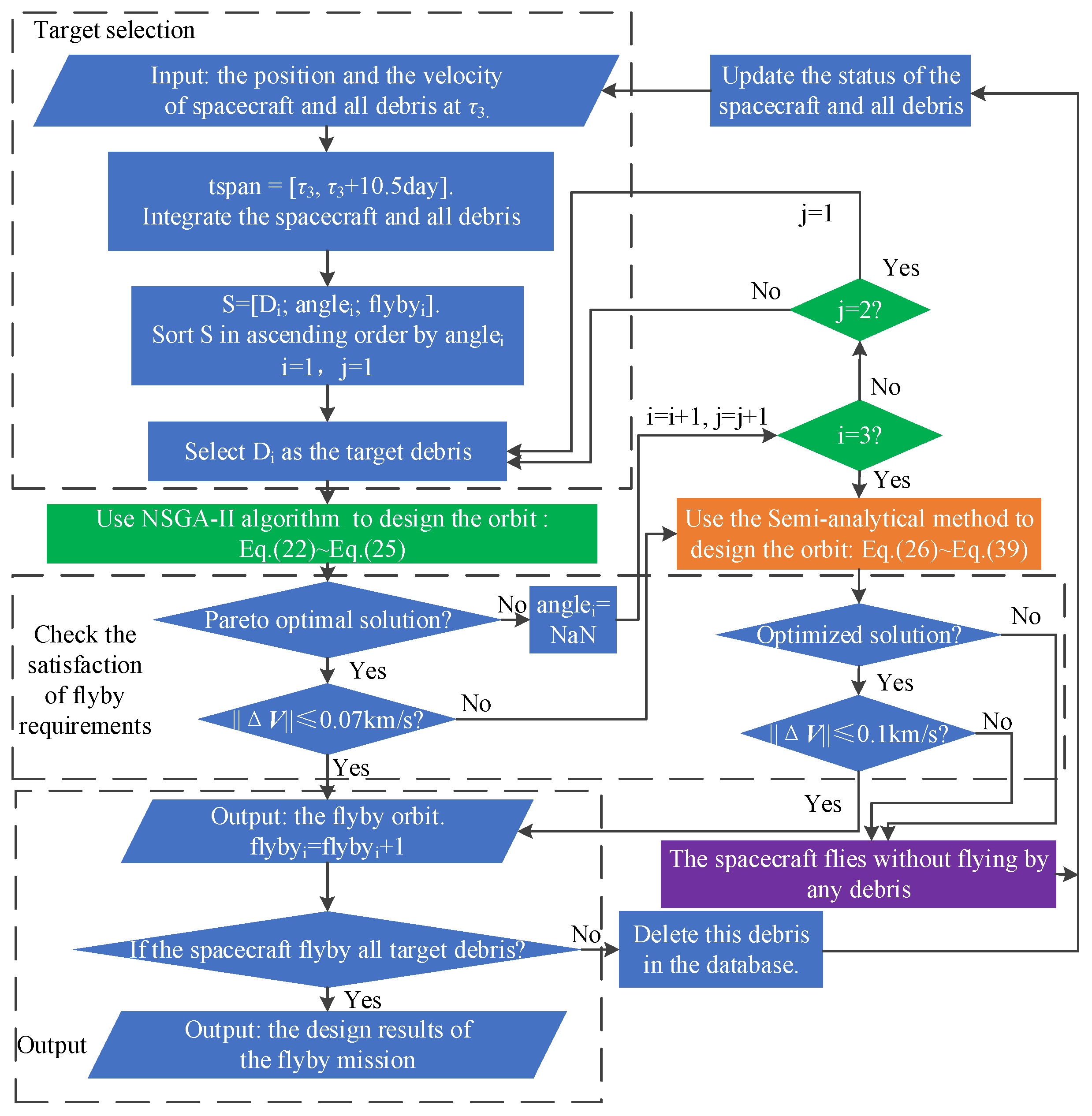
3. Target Selection of SSO Space Debris
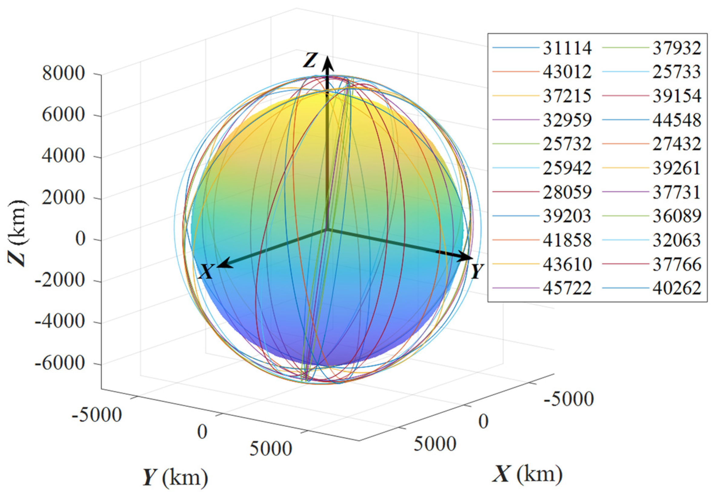
3.1. Analysis of SSO Space Debris
3.2. Selection of SSO Target Debris
- (1)
- The types of target debris are debris or rocket body.
- (2)
- The perigee altitude has not yet begun to decrease.
- (3)
- The target debris is generated by Changzheng rockets.
- (4)
- The radar cross-section area of the target is as follows: .
- (5)
- The mass of the target is as follows: .
- (6)
- , , and .
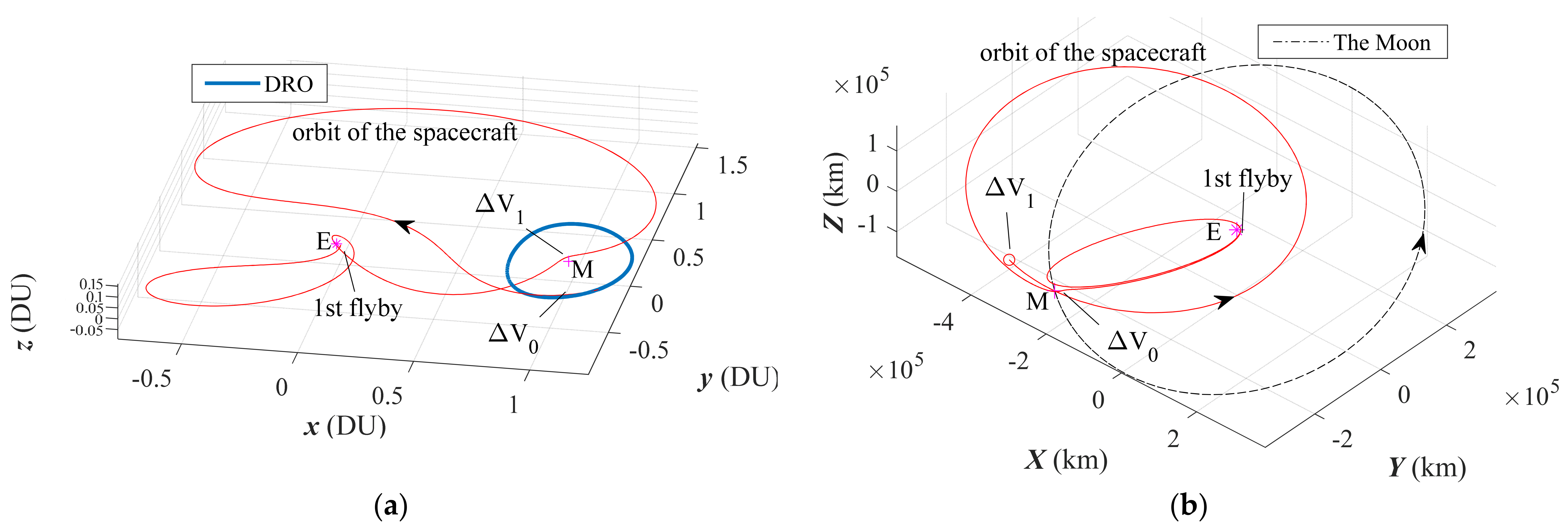
4. Phase 1: Two Impulses DRO–Earth Transfer Orbit Design
4.1. Single-Impulse DRO–Earth Transfer
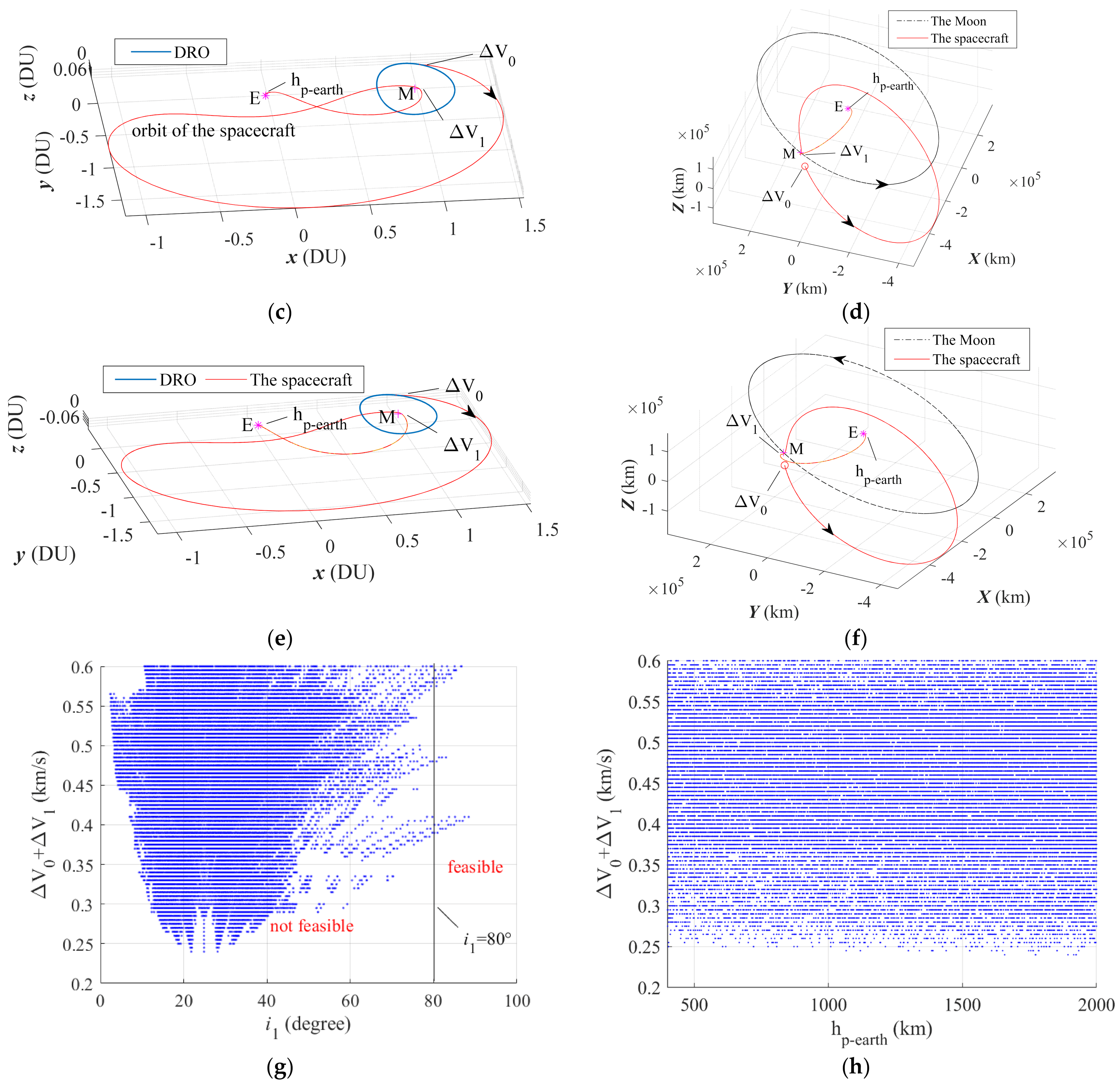
4.2. Two-Impulse DRO–Earth Transfer
4.3. Local Optimization
4.4. Optimal Result of Two-Impulse DRO–Earth Transfer
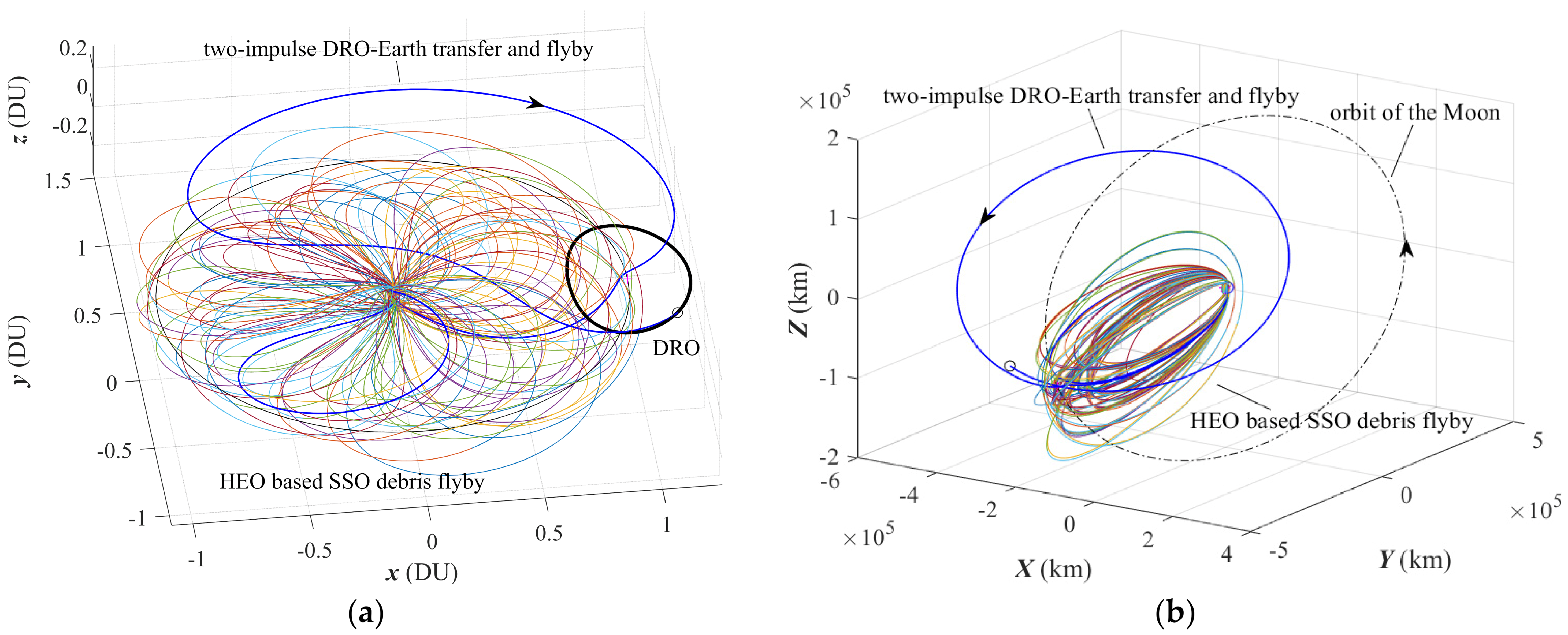
5. Phase 2: HEO Based SSO Objects Flyby
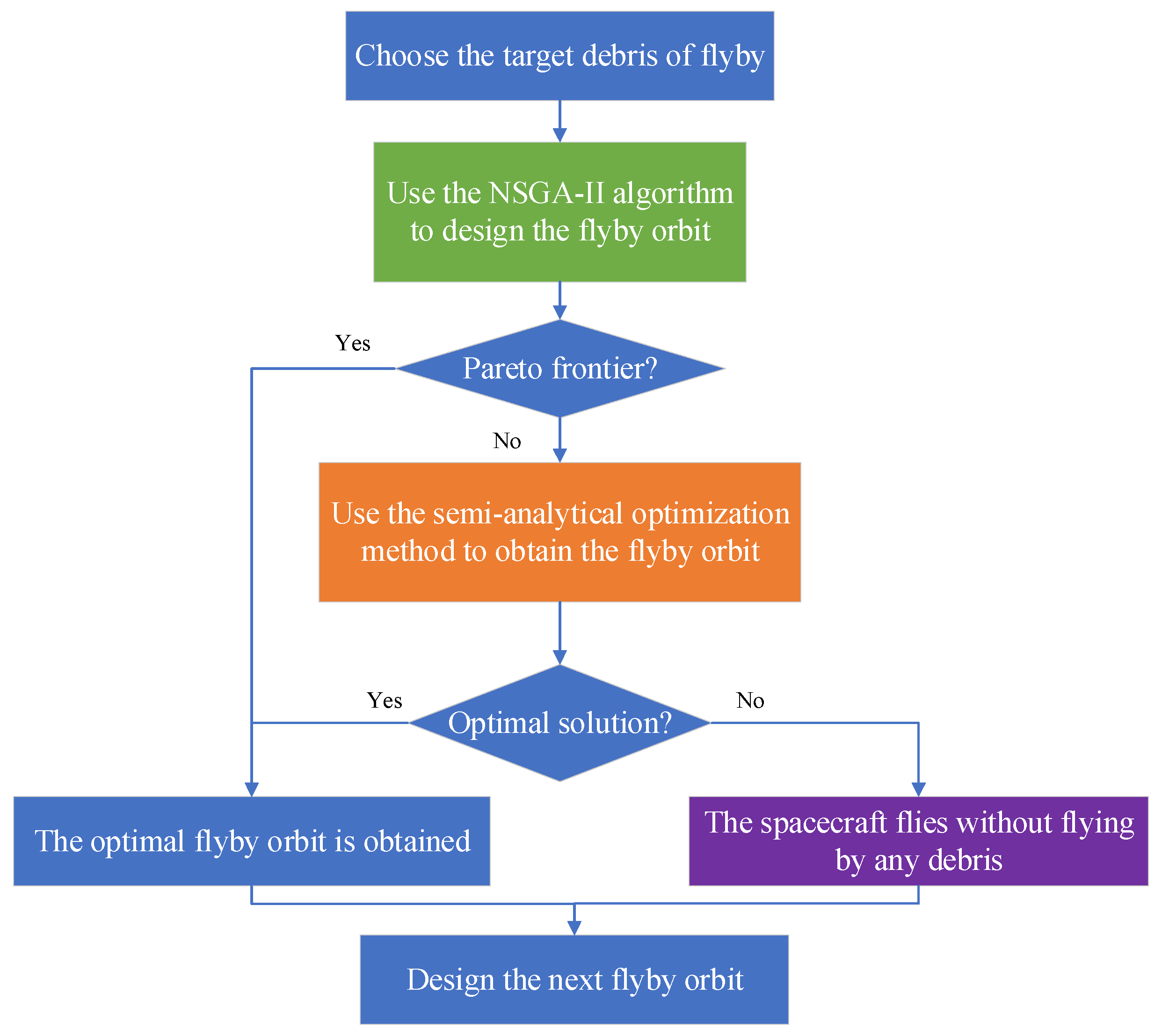
5.1. Multi-Objective Evolutionary Optimization Algorithm
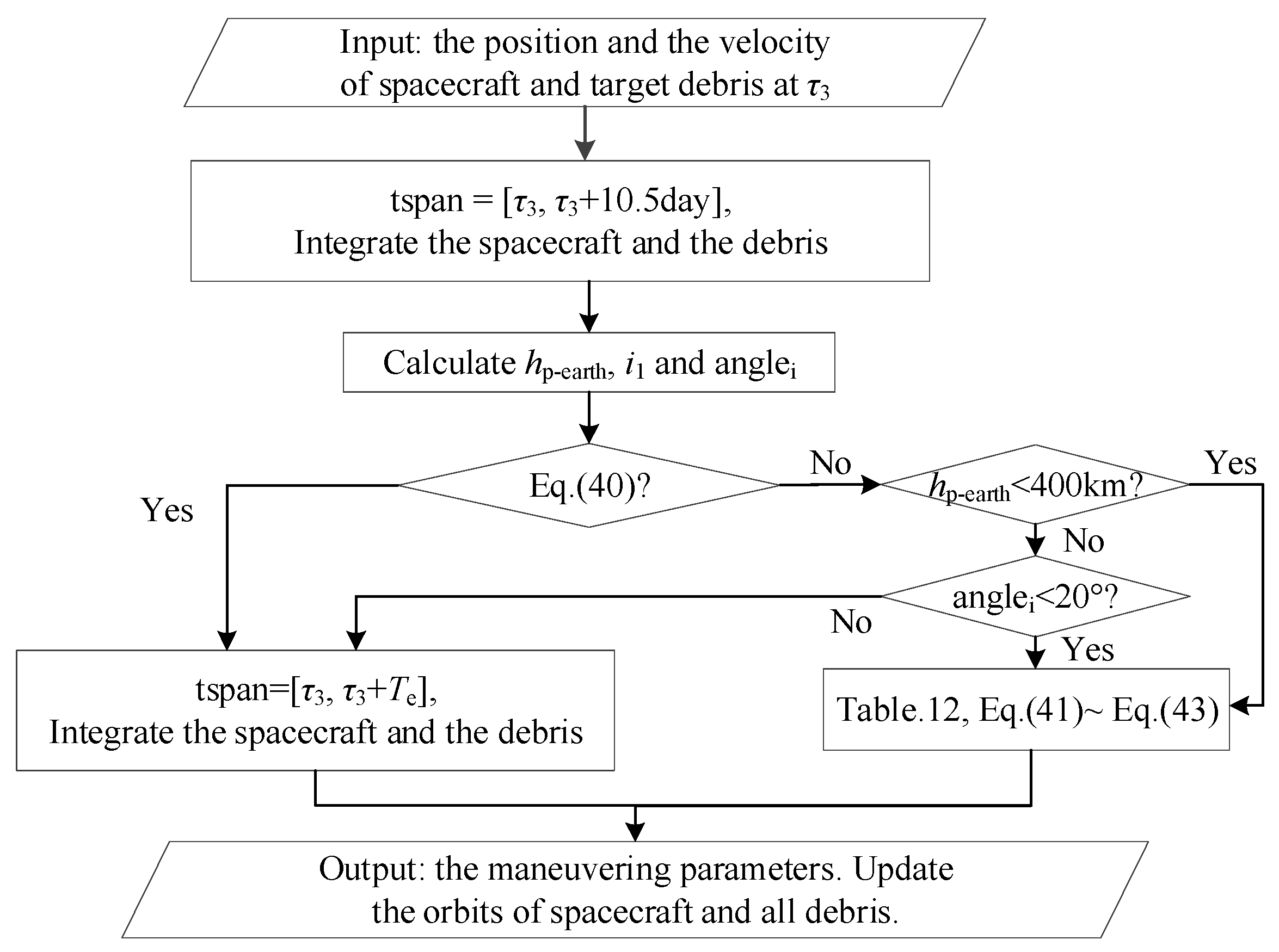
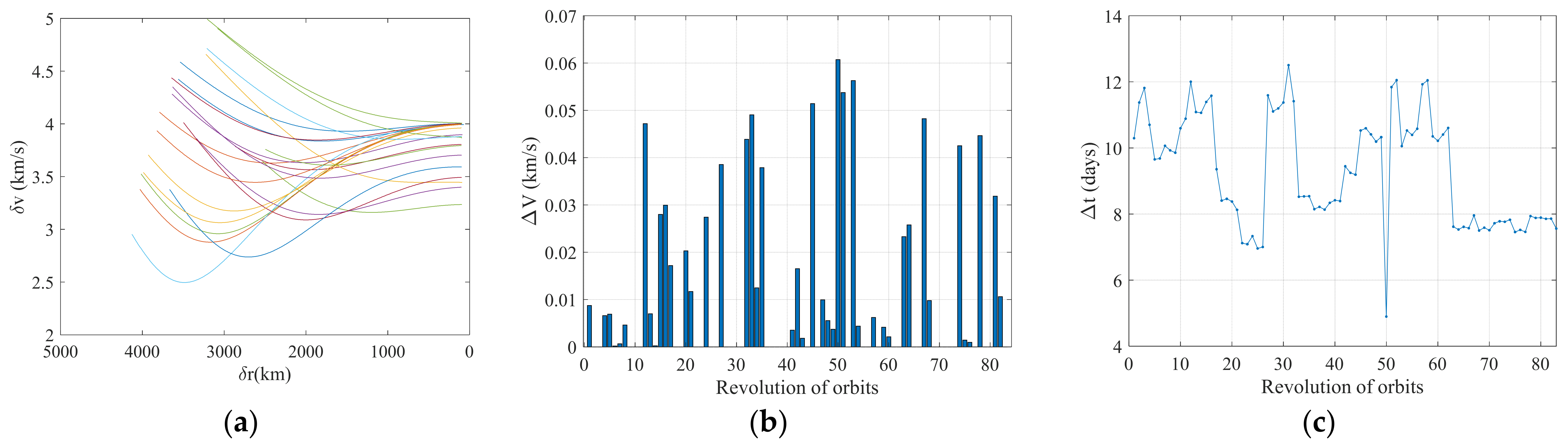
5.2. Semi-Analytical Optimization Method
6. Numerical Simulations and Analysis
7. Conclusions
Author Contributions
Funding
Data Availability Statement
Conflicts of Interest
Appendix A

| No. | NORAD Catalog Number | Type | Mass (kg) | Shape | Width (m) | Height (m) | Depth (m) | Diameter (m) | Span (m) | Max. Cross Section (m2) | Min. Cross Section (m2) |
|---|---|---|---|---|---|---|---|---|---|---|---|
| 1 | 25733 | Debris | 50 | cone | 2.9 | 1.0 | 2.90 | N/A | 2.90 | 6.61 | 1.45 |
| 2 | 43012 | Rocket Body | 1000 | cylinder | N/A | 1.92 | N/A | 2.90 | 2.90 | 8.63 | 5.56 |
| 3 | 37215 | Rocket Body | 1000 | cylinder | N/A | 7.50 | N/A | 2.90 | 2.90 | 22.73 | 6.60 |
| 4 | 32959 | Rocket Body | 1000 | cylinder | N/A | 7.50 | N/A | 2.90 | 2.90 | 22.73 | 6.60 |
| 5 | 25732 | Rocket Body | 1000 | cylinder | N/A | 6.20 | N/A | 2.90 | 6.20 | 19.15 | 6.60 |
| 6 | 25942 | Rocket Body | 1000 | cylinder | N/A | 7.50 | N/A | 2.90 | 7.50 | 22.73 | 6.60 |
| 7 | 28059 | Rocket Body | 1000 | cylinder | N/A | 7.50 | N/A | 2.90 | 7.50 | 22.73 | 6.60 |
| 8 | 27432 | Rocket Body | 1000 | cylinder | N/A | 6.20 | N/A | 2.90 | 6.20 | 19.15 | 6.60 |
| 9 | 39261 | Rocket Body | 1000 | cylinder | N/A | 7.50 | N/A | 2.90 | 2.90 | 22.73 | 6.60 |
| 10 | 32063 | Rocket Body | 1000 | cylinder | N/A | 7.50 | N/A | 2.90 | 7.50 | 22.73 | 6.60 |
| 11 | 31114 | Rocket Body | 3800 | cylinder | N/A | 8.40 | N/A | N/A | 8.40 | 29.48 | 8.81 |
| 12 | 39203 | Rocket Body | 3800 | cylinder | N/A | 8.40 | N/A | N/A | 8.4 | 29.48 | 8.81 |
| 13 | 43610 | Rocket Body | 3800 | cylinder | N/A | 9.94 | N/A | N/A | 9.94 | 34.44 | 8.81 |
| 14 | 45722 | Rocket Body | 3800 | cylinder | N/A | N/A | N/A | N/A | 7.49 | 26.59 | 8.81 |
| 15 | 37731 | Rocket Body | 3800 | cylinder | N/A | 8.40 | N/A | N/A | 8.40 | 29.48 | 8.81 |
| 16 | 36089 | Rocket Body | 3800 | cylinder | N/A | 8.40 | N/A | N/A | 8.40 | 29.48 | 8.80 |
| 17 | 37766 | Rocket Body | 3800 | cylinder | N/A | 8.40 | N/A | N/A | 8.40 | 29.48 | 8.81 |
| 18 | 40262 | Rocket Body | 3800 | cylinder | N/A | 8.40 | N/A | N/A | 8.40 | 29.48 | 8.81 |
| 19 | 44548 | Rocket Body | 4000 | cylinder | N/A | 8.90 | N/A | 3.35 | 8.90 | 31.09 | 8.81 |
| 20 | 41858 | Rocket Body | 4006 | cylinder | N/A | 8.00 | N/A | 3.35 | 8.00 | 28.21 | 8.81 |
| 21 | 37932 | Rocket Body | 4006 | cylinder | N/A | 8.00 | N/A | 3.35 | 8.00 | 28.21 | 8.81 |
| 22 | 39154 | Rocket Body | 4006 | cylinder | N/A | 8.00 | N/A | 3.35 | 8.00 | 28.21 | 8.81 |
| No. | NORAD Catalog Number | a (km) | e | i (°) | (°) | (°) | (°) |
|---|---|---|---|---|---|---|---|
| 1 | 25733 | 7215.45 | 0.001437 | 98.91 | 210.47 | 350.69 | 9.40 |
| 2 | 43012 | 7083.69 | 0.012716 | 98.73 | 186.11 | 344.70 | 15.04 |
| 3 | 37215 | 7115.79 | 0.008747 | 98.82 | 315.56 | 295.20 | 64.01 |
| 4 | 32959 | 7130.70 | 0.006916 | 98.90 | 131.89 | 282.58 | 87.49 |
| 5 | 25732 | 7211.30 | 0.003646 | 98.90 | 210.33 | 233.36 | 178.63 |
| 6 | 25942 | 7149.59 | 0.009876 | 98.80 | 157.51 | 194.49 | 224.30 |
| 7 | 28059 | 7095.13 | 0.005130 | 98.50 | 100.61 | 86.59 | 274.12 |
| 8 | 27432 | 7223.48 | 0.005012 | 99.08 | 193.56 | 195.95 | 221.49 |
| 9 | 39261 | 7159.09 | 0.003200 | 98.96 | 341.92 | 8.18 | 351.99 |
| 10 | 32063 | 7103.01 | 0.005454 | 97.97 | 177.71 | 279.44 | 140.95 |
| 11 | 31114 | 7205.63 | 0.005846 | 98.23 | 4.81 | 274.66 | 84.79 |
| 12 | 39203 | 7087.82 | 0.005101 | 98.47 | 359.04 | 345.25 | 14.73 |
| 13 | 43610 | 7090.60 | 0.009093 | 98.57 | 285.13 | 148.48 | 212.19 |
| 14 | 45722 | 7116.03 | 0.005192 | 98.59 | 125.23 | 20.02 | 340.30 |
| 15 | 37731 | 7024.18 | 0.006011 | 97.65 | 180.41 | 152.27 | 20.73 |
| 16 | 36089 | 7104.23 | 0.008140 | 98.20 | 148.55 | 196.06 | 222.06 |
| 17 | 37766 | 7050.14 | 0.00444 | 98.33 | 58.18 | 242.68 | 116.99 |
| 18 | 40262 | 7035.01 | 0.004633 | 98.30 | 330.04 | 137.72 | 222.76 |
| 19 | 44548 | 7139.02 | 0.000605 | 98.13 | 170.97 | 262.86 | 97.19 |
| 20 | 41858 | 7150.19 | 0.003359 | 98.50 | 159.81 | 184.49 | 175.60 |
| 21 | 37932 | 7196.48 | 0.003811 | 98.69 | 111.14 | 108.96 | 262.11 |
| 22 | 39154 | 7020.85 | 0.002062 | 98.41 | 55.43 | 88.48 | 271.88 |
References
- NASA Webpage. Orion Will Go the Distance in Retrograde Orbit During Artemis I. Available online: https://www.nasa.gov/missions/orion-will-go-the-distance-in-retrograde-orbit-during-artemis-i/ (accessed on 2 February 2023).
- NASA Webpage. Meet NASA’s Orion Spacecraft. Available online: https://www.nasa.gov/missions/meet-nasas-orion-spacecraft/ (accessed on 2 February 2023).
- Broucke, R. NASA Technical Report 32-1168: Periodic Orbits in the Restricted Three-Body Problem with Earth-Moon Masses; Jet Propulsion Laboratory, California Institute of Technology: Pasadena, CA, USA, 1968.
- Bezrouk, C.J.; Parker, J. Long duration stability of distant retrograde orbits. In Proceedings of the AIAA/AAS Astrodynamics Specialist Conference, San Deiego, CA, USA, 4–7 August 2014. [Google Scholar] [CrossRef]
- Strange, N.; Landau, D.; McElrath, T.; Lantoine, G.; Lam, T.; McGuire, M.; Burke, L.; Martini, M.; Dankanich, J. Overview of mission design for NASA asteroid redirect robotic mission concept. In Proceedings of the 33rd International Electric Propulsion Conference, Washington, DC, USA, 6–10 October 2013. [Google Scholar]
- Bezrouk, C.J.; Parker, J. Long term evolution of distant retrograde orbits in the Earth-Moon system. Astrophys. Space Sci. 2017, 326, 176. [Google Scholar] [CrossRef]
- Welch, C.M.; Parker, J.S.; Buxton, C. Mission Considerations for Transfers to a Distant Retrograde Orbit. J. Astronaut. Sci. 2015, 62, 101–124. [Google Scholar] [CrossRef]
- Murakami, N.; Yamanaka, K. Trajectory design for rendezvous in lunar distant retrograde orbit. In Proceedings of the 2015 IEEE Aerospace Conference, Big Sky, MT, USA, 7–14 March 2015; pp. 1–13. [Google Scholar] [CrossRef]
- Demeyer, J.; Gurfil, P. Transfer to small distant retrograde orbits. In Proceedings of the American Institute of Physics Conference, Greensboro, NC, USA, 1–2 August 2007; pp. 20–31. [Google Scholar] [CrossRef]
- Capdevila, L.; Guzzetti, D.; Howell, K. Various transfer options from Earth into distant retrograde orbits in the vicinity of the Moon. Adv. Astronaut. Sci. 2014, 118, 3659–3678. [Google Scholar]
- Ren, J.; Li, M.; Zheng, J. Families of transfers from the Moon to distant retrograde orbits in cislunar space. Astrophys. Space Sci. 2020, 365, 192. [Google Scholar] [CrossRef]
- Xu, M.; Xu, S. Exploration of distant retrograde orbits around Moon. Acta Astronaut. 2009, 65, 853–860. [Google Scholar] [CrossRef]
- Zhang, R.; Wang, Y.; Zhang, C.; Zhang, H. The transfers from lunar DROs to Earth orbits via optimization in the four body problem. Astrophys. Space Sci. 2021, 366, 49. [Google Scholar] [CrossRef]
- Wen, C.; Gao, Y. Reachability study for spacecraft maneuvering from a distant retrograde orbit in the Earth-Moon system. In Proceedings of the 18th Australian International Aerospace Congress, Melbourne, Australia, 24–28 February 2019. [Google Scholar]
- Aixue, W.; Chen, Z.; Wang, S.; Zhang, H. Design considerations for access in to Earth-Moon DROs with lunar free-return trajectory. Manned Spacefl. 2022, 28, 81–89. (In Chinese) [Google Scholar] [CrossRef]
- Zeng, H.; Li, Z.; Peng, K.; Wang, P.; Huang, Z. Research on application of Earth-Moon NRHO and DRO for Lunar exploration. J. Astronaut. 2020, 41, 910–919. [Google Scholar] [CrossRef]
- Capdevila, L.R.; Howell, K.C. A transfer network linking Earth, Moon and the triangular libration point regions in the Earth-Moon system. Adv. Space Res. 2018, 62, 1826–1852. [Google Scholar] [CrossRef]
- Morand, V.; Dolado-Perez, J.-C.; Philippe, T.; Handschuh, D.-A. Mitigation rules compliance in low Earth orbit. J. Space Saf. Eng. 2014, 1, 84–92. [Google Scholar] [CrossRef]
- PARABOLIC ARC Webpage. NASA ODPO’s Large Constellation Study. Available online: http://34.196.180.244/2018/09/25/nasa-odpos-large-constellation-study/ (accessed on 29 December 2023).
- Liou, J.; Johnsonb, N. Instability of the present LEO satellite populations. Adv. Space Res. 2008, 41, 1046–1053. [Google Scholar] [CrossRef]
- Wormnes, K.; Le Letty, R.; Summerer, L.; Schonenborg, R.; Dubois-Matra, O.; Luraschi, E.; Cropp, A.; Krag, H.; Delaval, J. ESA technologies for space debris remediation. In Proceedings of the 6th European Conference on Space Debris, ESA Communications ESTEC Noordwijk, Daemstadt, Germany, 22–25 April 2013; pp. 85–92. [Google Scholar]
- Botta, E.; Sharf, I.; Misra, A.K. Evaluation of net capture of space debris in multiple mission scenarios. In Proceedings of the 26th AAS/AIAA Space Flight Mechanics Meeting, Napa, CA, USA, 14–18 February 2016. [Google Scholar]
- Nikolajsen, J.A.; Kristense, A.S. Self-deployable drag sail folded nine times. Adv. Space Res. 2021, 68, 4242–4251. [Google Scholar] [CrossRef]
- Underwood, C.; Viquerat, A.; Schenk, M.; Taylor, B.; Massimiani, C.; Duke, R.; Stewart, B.; Fellowes, S.; Bridges, C.; Aglietti, G.; et al. Inflatesail deorbit flight demonstration results and follow-on dragsail applications. Acta Astronaut. 2019, 162, 344–358. [Google Scholar] [CrossRef]
- Bekey, I. Tethers open new space options. Astronaut. Aeronaut. 1983, 21, 32–40. [Google Scholar]
- King, L.B.; Parker, G.G.; Deshmukh, S.; Chong, J.-H. Spacecraft Formation-Flying Using Inter-Vehicle Coulomb Forces; Technique Report; NASA Institute for Advanced Concepts: Atlanta, GA, USA, 2002.
- Monroe, D.K. Space debris removal using a high-power ground-based laser. In Proceedings of the Space Programs and Technologies Conference and Exhibit, Huntsville, AL, USA, 21–23 September 1993; pp. 276–283. [Google Scholar] [CrossRef]
- Kofford, S. System and Method for Creating an Artificial Atmosphere for the Removal of Space Debris. U.S. Patent US2013/0082146A1, 4 April 2013. [Google Scholar]
- Andrenucci, M.; Pergola, P.; Ruggiero, A. Active Removal of Space Debris Expanding Foam Application for Active Debris Removal; Technical Report; ESA Advanced Concepts Team: Noordwijk, The Netherlands, 2011. [Google Scholar]
- Hughes, J.; Schaub, H. Prospects of using a pulsed electrostatic tractor with nominal geosynchronous conditions. IEEE Trans. Plasma Sci. 2017, 45, 1887–1897. [Google Scholar] [CrossRef]
- Hammert, J.; Schaub, H. Debris attitude effects on electrostatic tractor relative motion control performance. In Proceedings of the 2021 AAS/AIAA Astrodynamics Specialist Conference, Big Sky, MT, USA, 8 August 2021. [Google Scholar]
- Rubenchik, A.M.; Barty, C.P.J.; Beach, R.J.; Erlandson, A.C.; Caird, J.A. Laser systems for orbital debris removal. In Proceedings of the AIP Conference, Santa Fe, NM, USA, 18–22 April 2010; pp. 347–353. [Google Scholar] [CrossRef]
- Phipps, C.R. A laser-optical system to re-enter or lower low Earth orbit space debris. Acta Astronaut. 2014, 93, 418–429. [Google Scholar] [CrossRef]
- Gregory, D.A.; Mergen, J.-F. Space Debris Removal Using Upper Atmosphere and Vortex Generator. U.S. Patent US8657235B2, 25 February 2014. [Google Scholar]
- Dunn, M.J. Space Debris Removal. U.S. Patent US8800933B2, 12 August 2014. [Google Scholar]
- Pergola, P.; Ruggiero, A.; Andrenucci, M.; Olympio, J.; Summerer, L. Expanding foam application for active space debris removal systems. In Proceedings of the 62nd International Astronautical Congress, Cape Town, SA, USA, 27 September–1 October 2010. [Google Scholar]
- Castronuovo, M.M. Active space debris removal—A preliminary mission analysis and design. Acta Astronaut. 2011, 69, 848–859. [Google Scholar] [CrossRef]
- Tadini, P.; Tancredi, U.; Grassi, M.; Anselmo, L.; Pardini, C.; Francesconi, A.; Branz, F.; Maggi, F.I.; Lavagna, M.I.; DeLuca, L.T.; et al. Active debris multi-removal mission concept based on hybrid propulsion. Acta Astronaut. 2014, 103, 26–35. [Google Scholar] [CrossRef]
- Van der Pas, N.; Lousada, J.; Terhes, C.; Bernabeu, M.; Bauer, W. Target selection and comparison of mission design for space debris removal by DL’s advanced study group. Acta Astronaut. 2014, 102, 241–248. [Google Scholar] [CrossRef]
- Federici, L.; Zavoli, A.; Colasurdo, G. On the use of A* search for active debris removal mission planning. J. Space Saf. Eng. 2021, 8, 245–255. [Google Scholar] [CrossRef]
- De Bonis, A.; Angeletti, F.; Lannelli, P.; Gasbarri, P. Mixed kane-newton multi-body analysis of a dual-arm robotic system for on-orbit servicing missions. Aerotec. Missili Spazio 2021, 100, 375–386. [Google Scholar] [CrossRef]
- Schaub, H.; Junkins, J. Analytical Mechanics of Space Systems, 3rd ed.; American Institute of Aeronautics and Astronautics, Inc.: Reston, VA, USA, 2014; Chapter 10; p. 547. [Google Scholar] [CrossRef]
- Zhang, R.; Wang, Y.; Zhang, H.; Zhang, C. Transfers from distant retrograde orbits to low lunar orbits. Celest. Mech. Dyn. Astron. 2022, 132, 41. [Google Scholar] [CrossRef]
- Zhang, R.; Wang, Y.; Shi, Y.; Zhang, C.; Zhang, H. Performance analysis of impulsive station-keeping strategies for cislunar orbits with the ephemeris model. Acta Astronaut. 2022, 198, 152–160. [Google Scholar] [CrossRef]
- Zhang, C.; Zhang, H. Lunar-gravity-assisted low-energy transfer from Earth into DROs. Acta Aeronaut. Astronaut. Sin. 2022, 44, 326507. (In Chinese) [Google Scholar] [CrossRef]
- Tselousova, A.; Shirobokov, M.; Trofimov, S. Direct two-impulse transfer from a low-Earth orbit to high circular polar orbits around the Moon. AIP Conf. Proc. 2019, 2171, 130022. [Google Scholar] [CrossRef]
- Anthony, W.; Larsen, A.; Butcher, E.A.; Parker, J.S. Impulsive guidance for optimal manifold-based transfers to Earth-Moon L1 halo orbits. In Proceedings of the 23rd AAS/AIAA Spaceflight Mechanics Meeting, Kauai, HI, USA, 10–14 February 2013. [Google Scholar]
- Conte, D.; He, G.-W.; Spencer, B.; Melton, G. Trajectory design for LEO to lunar Halo orbits using manifold theory and fireworks optimization. In Proceedings of the 2018 AAS/AIAA Astrodynamics Specialist Conference, Snowbird, UT, USA, 19–23 August 2018. [Google Scholar]
- United Nations Office for Outer Space Affairs. Guidelines for the Long-Term Sustainability of Outer Space Activities. Available online: https://www.unoosa.org/res/oosadoc/data/documents/2019/aac_105c_1l/aac_105c_1l_366_0_html/V1805022.pdf (accessed on 2 February 2023).
- Shah, V.; Beeson, R.; Coverstone, V. A method for optimizing low-energy transfer in the Earth-Moon system using global transport and genetic algorithms. In Proceedings of the AIAA/AAS Astrodynamics Specialist Conference, Long Beach, CA, USA, 13–16 September 2016. [Google Scholar]
- Battin, R.H. An Introduction to the Mathematics and Methods of Astrodynamics, revised ed.; American Institute of Aeronautics and Astronautics Press: Reston, VA, USA, 2001; Chapter 11; p. 443. ISBN 978-7-5159-1488-6. [Google Scholar]
- Chase, J.P.; Chow, N.; Gralla, E.; Kasdin, N.J. LEO constellation design using the lunar L1 point. In Proceedings of the AAS/AIAA Space Flight Mechanics Meeting, Maui, HI, USA, 8–12 February 2004. [Google Scholar]
- Nadoushan, M.J.; Novinzadeh, A.B. Satellite constellation build-up via three-body dynamics. J. Aerosp. Eng. 2013, 228, 155–160. [Google Scholar] [CrossRef]
- Carletta, S. A single-launch deployment strategy for lunar constellations. Appl. Sci. 2023, 13, 5104. [Google Scholar] [CrossRef]
- CelesTrack Webpage. Satellite Catalog (SATCAT). Available online: https://celestrak.org/satcat/search.php (accessed on 26 February 2024).


| Target Orbits | ||ΔVtotal|| | Types of Transfer |
|---|---|---|
| DRO | 3.1934 km/s [45] | Lunar gravity assist and weak stability boundary |
| GEO | 4.2457 km/s [45] | Direct two impulses |
| PLO | 3.8 km/s [46] | Direct two impulses |
| NRHO | 4 km/s [46] | Direct two impulses |
| L1 halo orbit | 3.61 km/s [47] | Two impulses and stable manifold |
| L2 halo orbit | 3.36 km/s [48] | Two impulses and stable manifold |
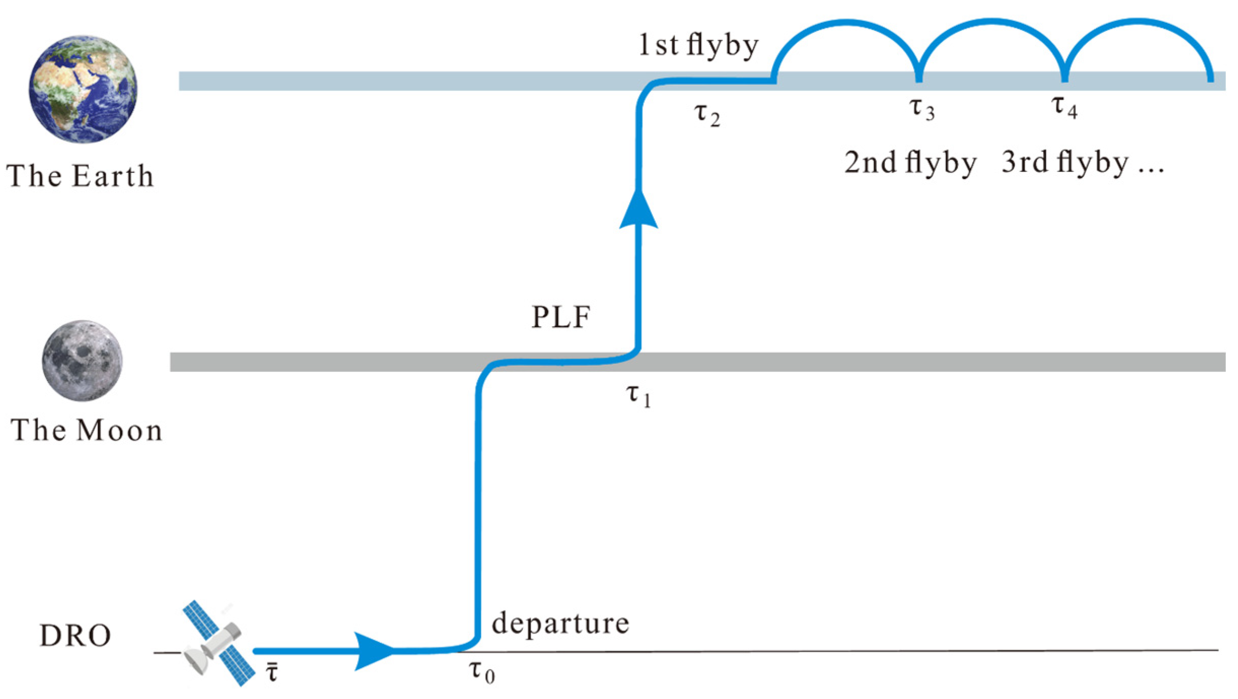
| Steps | Description |
|---|---|
| Step 1 | At (chosen as 2025/10/1/00:00:00), the spacecraft is located in DRO. The initial phase is 0°. = 2025/11/1/00:00:00. |
| Step 2 | At ( < < ), the spacecraft applies an impulse ΔV0 and leaves DRO, flying towards the Moon. |
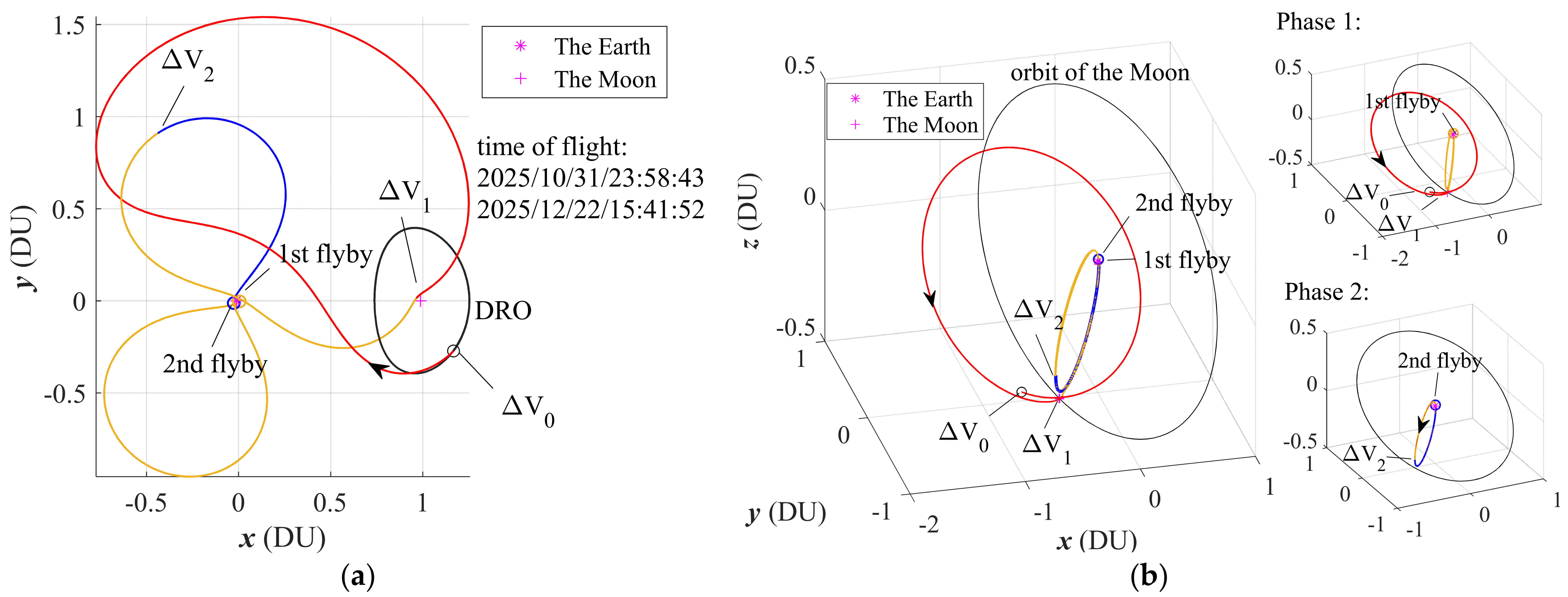
| Step 3 | The spacecraft enters the Moon’s sphere of influence. At , the spacecraft applies an impulse ΔV1 and accomplishes a powered lunar flyby transfer (PLF). The spacecraft enters the Moon–Earth transfer orbit. Then, at , the spacecraft near-coplanar flies by a piece of SSO space debris near the perigee. |
| Step 4 | The spacecraft flies towards to the apogee. To implement orbit phasing and adjust the orbit, the spacecraft applies an impulse ΔV2 near the apogee. As a result, the spacecraft can near-coplanar fly by the next piece of SSO space debris when the spacecraft is close to the perigee. |
| Step 5 | The spacecraft repeats Step 4 until all of the space debris in the database have been flown by at least once. |
| Parameters | Meaning | Requirement |
|---|---|---|
| Days between and | ||
| The transfer time from DRO to the perilune | ||
| The transfer time from the perilune to near the perigee | ||
| The modulus of | ||
| The modulus of | ||
| The modulus of impulse applied in HEO | ||
| The period of HEO | HEO is resonant with the Moon | |
| The height of perilune | ||
| The height of perigee | ||
| The distance of the flyby | ||
| The magnitude of the relative flyby velocity |
| Parameters | Meaning | Range of Ergodicity |
|---|---|---|
| Days between and | The sweep interval is [1, ] days. The sweep stepsize is . | |
| The modulus of | The sweep interval is [0.005, ] km/s. The sweep stepsize is . | |
| Two direction angles of | The sweep interval is [0° 360°]. The sweep stepsize is . |
| Colors of Box | (day) | (km/s) | () (°) | (km) | (°) | (°) | (°) | (°) | |
|---|---|---|---|---|---|---|---|---|---|
| red, Figure 6a | 23 | 0.3650 | (80,0) | 224,818 | 0.78 | 38.97 | 348.60 | 319.72 | 240.08 |
| 23 | 0.3650 | (100,180) | 224,818 | 0.78 | 38.97 | 348.60 | 319.72 | 240.08 | |
| blue, Figure 6a | 24 | 0.3950 | (240,180) | 217,626 | 0.85 | 46.97 | 350.77 | 342.92 | 202.02 |
| 24 | 0.3950 | (300,0) | 217,626 | 0.85 | 46.97 | 350.77 | 342.92 | 202.02 | |
| red, Figure 6b | 11 | 0.1850 | (190,40) | 221,927 | 0.82 | 57.17 | 351.40 | 161.45 | 226.10 |
| 11 | 0.1850 | (350,220) | 221,927 | 0.82 | 57.17 | 351.40 | 161.45 | 226.10 | |
| blue, Figure 6b | 9 | 0.1100 | (190,130) | 197,036 | 0.86 | 52.04 | 356.46 | 162.54 | 218.22 |
| 9 | 0.1100 | (350.310) | 197,036 | 0.86 | 52.04 | 356.46 | 162.54 | 218.22 |
| Epoch | (km) | (°) | (°) | (°) | (°) | |
|---|---|---|---|---|---|---|
| When spacecraft enters the Moon’s SOI | 373,802 | 0.69 | 20.98 | 7.04 | 3.20 | 296.40 |
| When spacecraft exits the Moon’s SOI | 209,944 | 0.82 | 62.71 | 43.32 | 9.93 | 248.97 |
| Parameters | Meaning | Range of Ergodicity |
|---|---|---|
| The first maneuver | of each in set | |
| The modulus of | The sweep interval is [0.005, ] km/s. The sweep stepsize is . | |
| Two direction angles of | The sweep interval is . The sweep stepsize is . |
| Colors of Box | (km/s) | () (°) | (km) | (°) | (°) | (°) | (°) | |
|---|---|---|---|---|---|---|---|---|
| red, Figure 8a | 0.2000 | (120, 90) | 118,588 | 0.94 | 13.69 | 114.27 | 235.944 | 0.00 |
| 0.2000 | (60, 270) | 118,588 | 0.94 | 13.69 | 114.27 | 235.944 | 0.00 | |
| blue, Figure 8a | 0.2000 | (240, 90) | 118,587 | 0.94 | 53.82 | 355.67 | 348.26 | 359.99 |
| 0.2000 | (300, 270) | 118,587 | 0.94 | 53.82 | 355.67 | 348.26 | 359.99 | |
| red, Figure 8b | 0.1550 | (230, 170) | 119,701 | 0.94 | 43.35 | 359.40 | 347.98 | 0.00 |
| 0.1550 | (310, 350) | 119,701 | 0.94 | 43.35 | 359.40 | 347.98 | 0.00 | |
| blue, Figure 8b | 0.2000 | (300, 260) | 125,231 | 0.94 | 51.05 | 356.39 | 347.44 | 359.99 |
| 0.2000 | (240, 80) | 125,231 | 0.94 | 51.05 | 356.39 | 347.44 | 359.99 |
| Parameters | /days | /days | /days | Flyby Debris | ||||
|---|---|---|---|---|---|---|---|---|
| DRO | ||||||||
| 3:2 resonance | 285.0 | 27.46 | 185.0 | 13.89 | 470.0 | 41.35 | 25733 | |
| 2:1 resonance | 371.2 | 28.02 | 185.7 | 3.85 | 556.9 | 31.87 | 37766 | |
| 3:1 resonance | 365.0 | 26.67 | 165.0 | 13.92 | 530.0 | 40.59 | 32959 | |
| Departure Time | /° | /days | /days | Flyby Debris | /km | |||
|---|---|---|---|---|---|---|---|---|
| 2025/10/31/23:58:43 | 236.70 | 285.0 | 27.46 | 185.0 | 13.89 | 25733 | 69.75 | 3.99 |
| Population Size | Maximum Iterations | Simulates Binary Crossover Parameters | Polynomial Mutation Parameter | Probability of Mutation | Probability of Crossover |
|---|---|---|---|---|---|
| 1500 | 150 | 20 | 100 | 0.2 | 1 |
| Parameters | Meaning |
|---|---|
| The modulus of the impulse . | |
| is the angle between and the projection of in the plane, and is the angle between the projection of in the plane and . | |
| Time from the flyby point of the previous revolution to the moment of maneuver in the current revolution. | |
| Time from the moment of maneuver to fly by the target debris. |
| Revolution of Orbits | Target Debris | /rad | /rad | /day | /day | /km | ||
|---|---|---|---|---|---|---|---|---|
| 1 | 25732 | 8.74 | 6.26 | 0.59 | 4.03 | 6.27 | 99.04 | 4.00 |
| 2~3 | / | / | / | / | / | 23.19 | / | / |
| 4 | / | 6.61 | 4.16 | 0.11 | 4.37 | 10.70 | / | / |
| 5 | / | 6.92 | 4.85 | 3.28 | 3.03 | 6.62 | / | / |
| 6 | 45722 | 0.16 | 4.80 | 0.52 | 0.00 | 9.68 | 100.00 | 3.90 |
| 7 | / | 0.65 | 1.07 | 6.27 | 0.00 | 10.06 | / | / |
| 8 | / | 4.60 | 2.08 | 2.23 | 4.99 | 4.93 | / | / |
| 9~11 | / | / | / | / | / | 31.34 | / | / |
| 12 | / | 47.16 | 4.40 | 3.85 | 0.16 | 11.84 | / | / |
| 13 | 37766 | 7.00 | 4.78 | 1.92 | 6.61 | 4.48 | 99.91 | 4.00 |
| 14 | 32063 | 0.22 | 1.82 | 5.90 | 0.00 | 11.06 | 100.00 | 3.80 |
| 15 | 39261 | 28.00 | 0.93 | 3.94 | 5.71 | 5.68 | 100.00 | 4.00 |
| 16 | 39203 | 29.94 | 6.27 | 6.28 | 9.82 | 1.76 | 100.00 | 4.00 |
| 17 | / | 17.16 | 4.23 | 5.14 | 0.00 | 9.36 | / | / |
| 18~19 | / | / | / | / | / | 16.87 | / | / |
| 20 | 40262 | 20.29 | 1.04 | 2.00 | 3.99 | 4.38 | 93.04 | 3.44 |
| 21 | / | 11.69 | 4.45 | 1.70 | 8.13 | 0.00 | / | / |
| 22 | 43610 | / | / | / | / | 7.12 | 100.00 | 3.23 |
| 23 | / | / | / | / | / | 7.09 | / | / |
| 24 | / | 27.42 | 0.07 | 1.58 | 3.92 | 3.41 | / | / |
| 25~26 | / | / | / | / | / | 13.96 | / | / |
| 27 | 43012 | 38.55 | 1.71 | 4.67 | 0.00 | 11.59 | 100.00 | 3.96 |
| 28~31 | / | / | / | / | / | 46.18 | / | / |
| 32 | 27433 | 43.86 | 1.60 | 0.72 | 2.95 | 8.47 | 100.00 | 3.40 |
| 33 | 27432 | 49.03 | 0.12 | 2.11 | 0.10 | 8.42 | 100.00 | 3.86 |
| 34 | 25942 | 12.47 | 2.86 | 1.74 | 4.74 | 3.80 | 99.99 | 4.00 |
| 35 | / | 37.87 | 4.07 | 5.51 | 4.02 | 4.52 | / | / |
| 36~40 | / | / | / | / | / | 41.25 | / | / |
| 41 | 39154 | 3.54 | 5.38 | 2.25 | 1.78 | 6.61 | 100.00 | 3.49 |
| 42 | 28059 | 16.52 | 4.99 | 0.41 | 4.32 | 5.12 | 100.00 | 3.59 |
| 43 | / | 1.80 | 4.38 | 2.50 | 4.65 | 4.60 | / | / |
| 44 | / | / | / | / | / | 9.19 | / | / |
| 45 | / | 51.41 | 5.91 | 4.26 | 4.69 | 5.83 | / | / |
| 46 | / | / | / | / | / | 10.60 | / | / |
| 47 | 37932 | 9.95 | 4.44 | 4.88 | 4.10 | 6.31 | 100.00 | 4.00 |
| 48 | 36089 | 5.55 | 5.67 | 3.25 | 4.77 | 5.42 | 99.88 | 4.00 |
| 49 | 37731 | 3.71 | 2.84 | 5.29 | 4.04 | 6.28 | 100.00 | 3.70 |
| 50 | / | 60.70 | 4.22 | 0.12 | 0.00 | 4.90 | / | / |
| 51 | / | 53.77 | 0.87 | 0.00 | 0.00 | 11.84 | / | / |
| 52 | / | / | / | / | / | 12.05 | / | / |
| 53 | / | 56.27 | 0.81 | 4.09 | 0.40 | 9.65 | / | / |
| 54 | / | 4.39 | 0.99 | 5.22 | 5.29 | 5.23 | / | / |
| 55~56 | / | / | / | / | / | 20.97 | / | / |
| 57 | / | 6.20 | 2.16 | 4.51 | 11.93 | 0.00 | / | / |
| 58 | / | / | / | / | / | 12.04 | / | / |
| 59 | / | 4.16 | 4.22 | 2.13 | 5.21 | 5.14 | / | / |
| 60 | / | 2.14 | 5.23 | 2.97 | 5.10 | 5.11 | / | / |
| 61~62 | / | / | / | / | / | 21.01 | / | / |
| 63 | / | 23.31 | 5.32 | 3.56 | 0.00 | 7.62 | / | / |
| 64 | 32959 | 25.77 | 3.49 | 0.94 | 2.23 | 5.30 | 100.00 | 4.00 |
| 65~66 | / | / | / | / | / | 15.19 | / | / |
| 67 | / | 48.23 | 4.22 | 4.80 | 4.57 | 3.39 | / | / |
| 68 | 31114 | 9.80 | 3.89 | 4.22 | 4.45 | 3.05 | 99.98 | 3.88 |
| 69~73 | / | / | / | / | / | 38.36 | / | / |
| 74 | / | 42.51 | 5.21 | 2.23 | 3.91 | 3.92 | / | / |
| 75 | / | 1.44 | 4.24 | 3.49 | 3.73 | 3.73 | / | / |
| 76 | / | 0.97 | 5.18 | 4.91 | 3.78 | 3.74 | / | / |
| 77 | / | / | / | / | / | 7.46 | / | / |
| 78 | 39203 | 44.64 | 5.83 | 4.31 | 3.19 | 4.76 | 100.00 | 4.00 |
| 79~80 | / | / | / | / | / | 15.77 | / | / |
| 81 | / | 31.86 | 5.19 | 2.49 | 3.86 | 4.00 | / | / |
| 82 | / | 10.62 | 5.98 | 5.97 | 3.61 | 4.25 | / | / |
| 83 | 37215 | / | / | / | / | 7.56 | 99.99 | 3.79 |
Disclaimer/Publisher’s Note: The statements, opinions and data contained in all publications are solely those of the individual author(s) and contributor(s) and not of MDPI and/or the editor(s). MDPI and/or the editor(s) disclaim responsibility for any injury to people or property resulting from any ideas, methods, instructions or products referred to in the content. |
© 2024 by the authors. Licensee MDPI, Basel, Switzerland. This article is an open access article distributed under the terms and conditions of the Creative Commons Attribution (CC BY) license (https://creativecommons.org/licenses/by/4.0/).
Share and Cite
Zhang, S.; Wang, S. Multiple SSO Space Debris Flyby Trajectory Design Based on Cislunar Orbit. Universe 2024, 10, 145. https://doi.org/10.3390/universe10030145
Zhang S, Wang S. Multiple SSO Space Debris Flyby Trajectory Design Based on Cislunar Orbit. Universe. 2024; 10(3):145. https://doi.org/10.3390/universe10030145
Chicago/Turabian StyleZhang, Siyang, and Shuquan Wang. 2024. "Multiple SSO Space Debris Flyby Trajectory Design Based on Cislunar Orbit" Universe 10, no. 3: 145. https://doi.org/10.3390/universe10030145