Article

Mercury’s Bow Shock and Magnetopause Variations According to MESSENGER Data

by
Dmitry Nevsky
1,2,†,
Alexander Lavrukhin
1,*,† and
Igor Alexeev
1,†
1
Federal State Budget Educational Institution of Higher Education, M.V.Lomonosov Moscow State University, Skobeltsyn Institute of Nuclear Physics (SINP MSU), 1(2), Leninskie Gory, GSP-1, Moscow 119991, Russia
2
Faculty of Physics, M.V.Lomonosov Moscow State University, Leninskie Gory, Moscow 119991, Russia
*
Author to whom correspondence should be addressed.
These authors contributed equally to this work.
Universe 2024, 10(1), 40; https://doi.org/10.3390/universe10010040
Submission received: 15 November 2023 / Revised: 30 December 2023 / Accepted: 13 January 2024 / Published: 16 January 2024

Abstract

:
Using data from the MESSENGER spacecraft magnetometer that describes the magnetopause and the bow shock crossing points of the Mercury’s magnetosphere, we have calculated the parameters of the paraboloids of revolution approximating the obtained points. For each spacecraft orbit, the subsolar magnetopause and bow shock standoff distances were obtained, based on the paraboloid parameters for each crossing point. The dependences of the magnetopause and bow shock subsolar standoff distances on the Mercury’s position relative to the Sun have been obtained. These profiles agree with decreases of the solar wind plasma dynamic pressure and the interplanetary magnetic field strength with heliocentric distance. The variations of the interplanetary and magnetosheath magnetic field were investigated. The average subsolar magnetosheath thickness and the value of the magnetic field jump at the bow shock during the transition from the upstream interplanetary magnetic field region to the magnetosheath were obtained.

1. Introduction

The MESSENGER spacecraft orbited Mercury for four years (2011–2015). During this time, Mercury made 16 and a half orbits around the Sun, and the spacecraft’s onboard magnetometer continuously recorded the magnitude and magnetic field vector direction. These continuous series of data transmitted to Earth contain unique information about the structure of Mercury’s magnetosphere and its internal planetary magnetic field. Analysis of this information made it possible not only to determine the planetary dipole magnetic moment and the dipole displacement relative to the center of Mercury, but also to find the main parameters of magnetospheric current systems [1,2,3]. According to this data, the average distance from the dipole to the subsolar point at Mercury’s magnetopause is ∼ 1.45 R M [4], where R M = 2440 km is the radius of the planet. Short-term variations of the solar wind pressure and the interplanetary magnetic field (IMF), and the small size of Mercury’s magnetosphere, make its magnetosphere highly dynamic. During extreme events, when the solar wind pressure is especially high, the global compression of the magnetosphere leads to the fact that the solar wind can directly affect Mercury’s surface [5,6]. It is worth noting that no significant variations in Mercury’s dipole tilt, shift, or magnetic moment have been found [7].
The size of the magnetosphere is mostly controlled by the solar wind dynamic pressure P s w , which is inversely proportional to the square of the distance to the Sun, r h . For Mercury’s orbit, which has a large eccentricity ( r h = 0.307 AU at perihelion and r h = 0.467 AU at aphelion), this dependence is significant. In one Hermean year (88 days), P s w changes 2.31 times when comparing at perihelion and aphelion. In the first approximation, due to the balance of the solar wind dynamic pressure and the magnetospheric magnetic field pressure, the distance to the subsolar point of the magnetopause R s s is proportional to P s w 1 / 6 , if we assume that the magnetospheric field at the subsolar point is proportional to the dipole field [2]. As a result, R s s r h 1 / 3 , and should change by a factor of 1.15 in one Mercury year.
The change in the magnetopause subsolar distance at the perihelion and aphelion of Mercury’s orbit was first considered by the pressure balance equation of solar wind dynamic pressure from Explorers 33 and 35 with the dipolar field obtained from the Mariner-10 [8]. An average magnetopause subsolar distance has been estimated using Mariner-10 magnetopause crossings and conic section fitting [9]. The next estimations of subsolar distance variations were obtained with MESSENGER observations, using the Shue magnetopause shape [10] and the paraboloid of revolution and magnetopause crossing positions (1) from 23 March 2011 to 19 December 2011 [4], (2) from 24 March 2011 to 31 October 2014 [11], and (3) for the whole MESSENGER mission [12] using the same method for magnetopause crossings determination [4]. The next advancement was the usage of the non-symmetrical three-dimensional model of the magnetosphere’s surface [13] for consideration of the perpendicular shift of the observed coordinates of the magnetopause crossing points from the magnetosphere’s surface [14,15]. According to their results, a change in the IMF direction leads to the Mercury magnetosphere deformations of the same order of magnitude as changes in dynamic pressure. Mercury’s bow shock subsolar distance has been estimated using Mariner-10 data and conic section [9]; MESSENGER bow shock crossing positions from 23 March 2011 to 19 December 2011 and conic section [4], and for the whole MESSENGER mission with the same conic section [16].
In our work, we analyze the data obtained over the entire MESSENGER lifetime using the coordinates of the magnetopause and bow shock crossing points, determined in [12], and use our own method to calculate the magnetopause and the bow shock subsolar distances. Having these values, it is possible to estimate the magnetopause and bow shock subsolar distances variations, average Mercury subsolar magnetosheath thickness, and the average ratio of the dayside magnetosheath magnetic field to the interplanetary magnetic field. This can be important for future modeling of the magnetosheath magnetic field as well as for modeling the magnetopause flaring and for the calculation of planetary magnetospheric parameter variations, such as magnetotail flux.

2. Methodology for Variations Determination

To study the possible effects of magnetospheric variations, the most productive way is to consider the global magnetospheric spatial parameters—magnetopause standoff distance R s s and the bow shock R b s . Having crossing points of these surfaces for each spacecraft orbit, we can reconstruct the geometric shape of the considered surfaces and determine the values of the required parameters, R s s and R b s . Thus, using the average surface shape and the surface crossing point, we determine the “instantaneous” surface and its subsolar distance and study the variation of this global parameter of the magnetosphere, in contrast to the studies of crossing point deviation from the average surface shape [14,15], or fitting the crossing points close to perihelion and aphelion with the chosen surface shape [16]. This method of “instantaneous” surface has already been used for the determination of Mariner-10 magnetopause crossings, where the magnetopause surface was approximated by an ellipsoid of revolution [17], as well as in papers [11,12], where for each magnetopause position they computed R s s with the Shue magnetopause shape [10] under rotational symmetry and with an average flaring parameter α = 0.5 .
Note that neither the bow shock nor the magnetopause are stationary structures. Due to the change in the solar wind pressure, they will constantly change their position and shape. The magnetopause may exhibit Kelvin–Helmholtz instability [18]; a variety of different boundary layer effects will lead to the fact that its model shape will differ from the observed one due to the appearance of “waves” on the surface of the current sheet, which the spacecraft can cross several times. Also, the “double” magnetopause effect is known for Mercury [19,20], which occurs due to a significant fraction of exospheric ions, in particular N a + ions, the most common in the Hermean magnetosphere. Their Larmor radius is much larger than that of protons, and the surface of the magnetopause acquires a complex structure. Thus, spacecraft can cross each surface several times (at several close points), compared to one crossing of the model surface. These effects will contribute to the error in the determination of the crossing point coordinates and, thus, the surface parameters.
In this paper, we use the dataset of the bow shock and magnetopause crossings positions for all MESSENGER orbits [12], determined by the visual inspection of the magnetic field measurements [4,12]. On the magnetometer data, the boundary crossing looks like multiple crossings due to the processes described above; that is why the dataset contains two points—the first and last boundary crossings for each surface in the Mercury Solar Orbital ( M S O ) system, where the X axis is positive sunward, the Z axis is positive northward and coincides with the axis rotation of Mercury, and the Y axis is positive duskward, forming the right-handed coordinate system. Due to the significant eccentricity of the orbit, planetary orbital speed significantly varies during one orbit. Thus, the X M S O direction does not coincide with solar wind incident direction and one has to rotate the X and Y axes by the aberration angle. Orbital speed values have been obtained from the NASA Horizons website (https://ssd.jpl.nasa.gov/horizons/, access granted on 1 September 2023). The solar wind speed has been taken as equal to an average value of 400 km/s following the previous papers [11,21,22]. The main reason for it is that MESSENGER’s construction strongly limited the possibility of direct solar wind parameters measurements onboard the spacecraft. That is why we could use either solar wind parameters modeling,—which will strongly complicate the task by not giving the large increase in accuracy because of the small angle variations—or looking for the regular changes on large scales, which are relatively small and sometimes obscured by large fluctuations [23].
Also, for our analysis, it is necessary to select one crossing point of each boundary, so we chose the average between the first and the last crossings from the dataset [12] for each boundary crossing.
For comparison, we first consider different models of bow shock and magnetopause surfaces and fit them to all crossings in the Mercury solar-magnetospheric coordinate system M S M . In this system, the X axis is directed from the Mercury dipole center toward the Sun along the solar wind velocity, the Y axis is directed along the Mercury’s orbital velocity, and the X Z plane contains the dipole moment vector and is perpendicular to the Y axis forming the right-handed coordinate system. We take into account the dipole offset when converting the aberrated M S O coordinates into the M S M system.

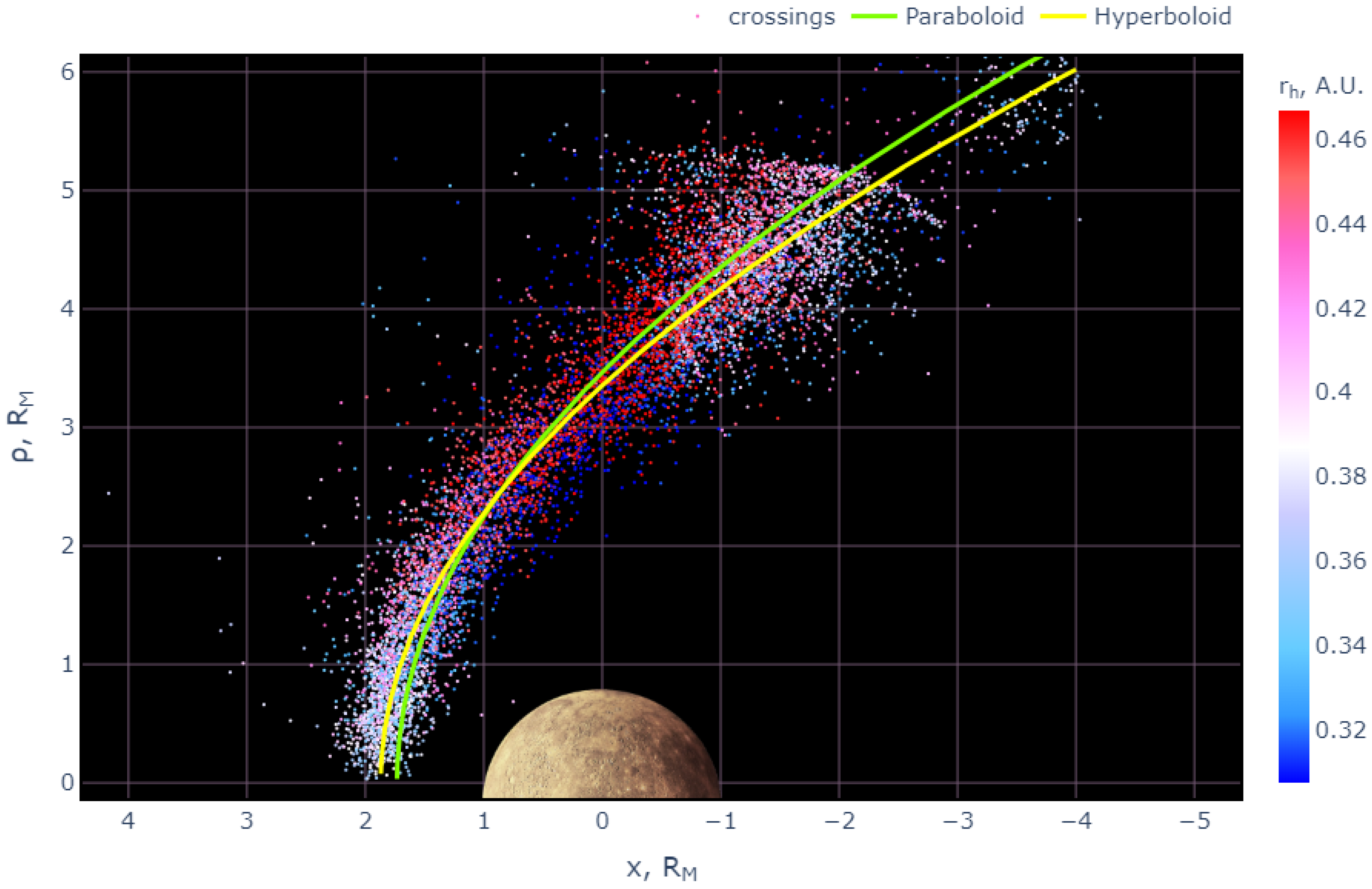
2.1. Bow Shock Surface Shape

The average shape of the bow shock can be described either by a paraboloid of revolution [24], or by a hyperboloid of a revolution [25], which transforms into a Mach cone at large distances. We compare both of these shapes in fitting the surface of the bow shock. The hyperboloid, as a conic section whose focus is free to lie along the X axis at X = X 0 , can be described by the following equation [25]:
( X X 0 ) 2 + Y 2 + Z 2 = L 1 + ε · cos θ ,
where the ε is the eccentricity and L is the semi-latus rectum, which determines the bow shock size in the terminator plane. The polar angle θ is measured from the + X axis about focus point X 0 to the radial vector, which is directed from the focus point to the crossing point. X , Y and Z are the crossing point coordinates. Optimal hyperboloid parameters have been taken from [12], where the best bow shock shape fit with varying L and ε parameters in the M S M coordinate system have been obtained. The best fit values for the parameters are: focal point X 0 = 0.4 R M , eccentricity ε = 1.02 , and focal parameter L = 3.03 R M . Also, these parameters have been obtained in [16], where authors, using the different bow shock crossings dataset and hyperboloid shape [25], obtained X 0 = 0.5067 R M , ε = 1.036 , L = 2.992 R M .
For the paraboloid fit of the bow shock, we use an equation with varying parabolic coordinate β b s and flaring parameter γ [26]:
Z R 1 β b s 2 + Y R 1 β b s 2 + 2 X R 1 = γ 2 + β b s 2 ,
where the bow shock subsolar point distance R b s = R 1 ( γ 2 + β b s 2 ) / 2 . From these equations, one can obtain R b s for each crossing point using the following equation:
R b s = ( Y 2 + Z 2 ) · ( 1 + γ 2 / β b s 2 ) 2 · X + X 2 + ( Y 2 + Z 2 ) · ( 1 + γ 2 / β b s 2 ) .
Figure 1 shows the results of the bow shock crossings fitting for all MESSENGER orbits with the mentioned surface shapes using the c u r v e _ f i t function from the s c i p y Python library (https://scipy.org/, access granted on 1 September 2023). A cloud of crossings points from [12] is shown. A point’s color depends on a heliocentric distance at the moment of crossing with red for points closer to aphelion to blue closer to perihelion with white at the middle. Parameter values for the best fit are R b s = 1.73 , β b s = 3.19 and γ = 1.1 × 10 5 . We will use these parameters for the determination of the instantaneous R b s for each crossing point.
If all points are normalized by the solar wind dynamic pressure, then the scatter of points will decrease. The cloud of points will become more compact, and fitting with different shapes will give a smaller standard deviation. Both hyperboloid and paraboloid shape fits describe the whole crossing points dataset well, especially in the nightside, but the obtained R b s = 1.73 R M value is lower than for the hyperboloid ( 1.89 R M ) and the average in the cloud of points.

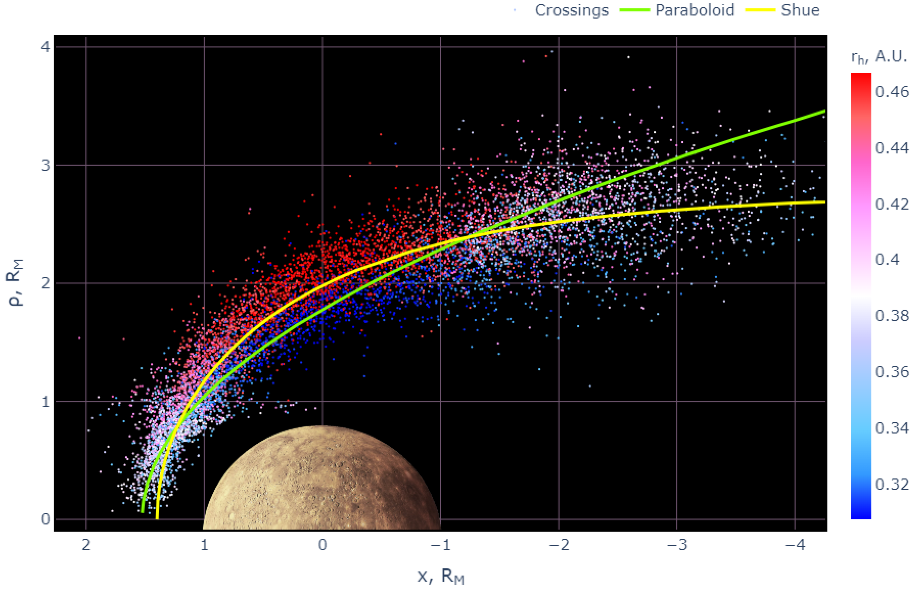
2.2. Magnetopause Surface Shape

The smoothed shape of Mercury’s magnetopause can be described both by axially symmetric shapes [10] and conic sections; in particular, a paraboloid of revolution, and a three-dimensional asymmetric surface containing depressions in the region of the cusp and magnetotail with different widths in the north–south and west–east directions [13]. From the whole variety of possible model surfaces, we chose the Shue shape [10], which has proven itself well at describing the Earth’s magnetosphere, and the shape of the paraboloid of revolution, used earlier for the determination of the magnetospheric parameters [1,2,27,28]. The three-dimensional asymmetric surface model [13] is closer to reality than the axially symmetric models, but it is quite difficult to distinguish the cusp region crossing from the dayside magnetopause crossing of a highly compressed magnetosphere that has one spacecraft in orbit. Thus, we chose the simpler axially symmetric models mentioned above. We do not impose restrictions on X M S M , as was the case in [13]; however, the spacecraft apoapsis naturally limits the extent of the used array in the nightside ( X M S M > 4 R M ). Also, we take into account crossings from all orbits, not excluding intervals during which coronal mass ejections were observed in the interplanetary space [29], as was carried out in previous works [15].
The subsolar distance R s s for the Shue model [10] is calculated with the following equation:
R s s = 2 1 + cos θ α X 2 + Y 2 + Z 2 ,
where θ = tan 1 ( Y 2 + Z 2 / X ) and α is the magnetotail flaring parameter with the optimal value to be 0.5 for Mercury’s case [4,12].
The surface of a paraboloid of revolution with a fixed parabolic coordinate β = β m = 1 and varying flaring parameter γ in the case of a magnetopause is defined as follows [26]:
Z R 1 2 + Y R 1 2 + 2 X R 1 = γ 2 + 1 ,
where the magnetopause subsolar point distance R s s = R 1 ( γ 2 + 1 ) / 2 . From these equations, one can obtain R s s for each crossing point using the following equation:
R s s = ( Y 2 + Z 2 ) ( γ 2 + 1 ) 2 · ( X + X 2 + ( Y 2 + Z 2 ) · ( γ 2 + 1 ) ) .
In Equation (5), X , Y and Z are the coordinates of the point of intersection of the magnetopause with the MESSENGER orbit, which, according to our assumption, is located on the paraboloid β m p = 1 with a distance from the dipole to the subsolar point R s s .
Figure 2 shows the results of the magnetopause crossings fitting for all MESSENGER orbits with the mentioned surface shapes. A cloud of magnetopause crossings points [12] is shown. The points’ color depends on a heliocentric distance at the moment of crossing with red for points close to aphelion to blue for those closer to perihelion, with white at the middle. Parameter values for the best fit are R s s = 1.52 , γ = 1.34 .
As can be seen from Figure 2, the paraboloid shape is unsatisfactory for describing the magnetopause’s surface beyond the distances X < 3 R M . Due to the fact that the algorithm also fits distant points, the [10] model better fits the average shape of the magnetopause. Thus, for the determination of the instantaneous R s s for each crossing point instead of the optimal γ = 1.34 obtained from fitting, we will use γ = 1 , which proved itself in describing the dayside magnetosphere, which is more important for determining the R s s [4,26]. It can also be seen that, at perihelion, the crossings points are, on average, slightly closer to the planet than at aphelion, that is, some dependence on the heliocentric distance is already visible here. The average value of R s s determined for the paraboloid of revolution is 1.52 R M , which is in good agreement with the estimate R s s = 1.45 R M [1,2] made by the χ 2 minimization method—the quadratic residual of the MESSENGER data and model formulas for the field along the spacecraft trajectory. This coincidence testifies in favor of both, completely different, methods of determining R s s .
To determine the variations of the magnetopause, we chose the surface of a paraboloid of revolution, despite the fact that the [10] surface better describes the average shape of the magnetopause. This is due to unification (the ability to apply the same type of dependence to describe different boundaries) and the further development of the obtained results—for example, for modeling the magnetosheath magnetic field in parabolic coordinates [30], assuming paraboloids of revolution for the shape of the magnetopause and of the bow shock, as well as in the global paraboloid model of Mercury ([1,2]). Also, variations of magnetopause location have already been calculated using the Shue magnetopause shape [10] and the ’instantaneous’ method in [12]; that is why, by applying the paraboloid magnetopause shape, we can compare the results to the Shue model approximation.

2.3. Magnetopause Flaring

When considering the R s s and R b s for the entire range of X M S M crossing points values, the artificial “observer” effect—associated with the local time of the spacecraft’s orbit plane—will arise. The MESSENGER trajectory is fixed relative to the planet, while the planet itself revolves around the Sun and, accordingly, the magnetosphere rotates around the Mercury body. Therefore, for half of the year, on the descending part of the trajectory, the spacecraft will cross the magnetosphere on the day side, and for half of the year on the night side. As a result, we obtain a bimodal distribution of distances, from dayside and tail crossings (Figure 3).
When constructing the surface of the instantaneous magnetopause containing the crossing point on the dayside, the most significant change is in R s s value, and flaring variations do not play a big role; in the case of approximating the crossing point located on the nightside, both factors are significant. Since the size of the paraboloid on the nightside is usually larger than the real magnetopause, the R s s calculated for the nightside crossing is always less than the R s s for the dayside crossing of the same orbit. Thus, to determine the R s s and also R b s variations, we consider crossing points only in the dayside magnetosphere. For the nightside crossings, the tail flaring contribution will be added to the R s s ( t ) and R b s ( t ) on the nightside, which will lead to an additional change in R s s ( t ) and R b s ( t ) .
If one calculates subsolar distances only for the ascending (or descending) part of the spacecraft’s orbit, much larger variations will be seen (Figure 3). When the spacecraft orbit plane passes through the terminator plane because of Mercury’s rotation around the Sun, the ascending (descending) part of the spacecraft orbit will cross the surface on the other side relative to the terminator plane, thus the flaring contribution will appear (for the nightside) or disappear (for the dayside). These passages of the terminator plane will be seen as jumps in the R s s ( t ) timeseries. This jump is caused, not by the real movement of the magnetopause at this moment, but by the mentioned “observer” effect—a feature of the spacecraft orbit passing through the terminator plane, thus receiving/losing the flaring’s contribution to the calculated distance.

3. Results

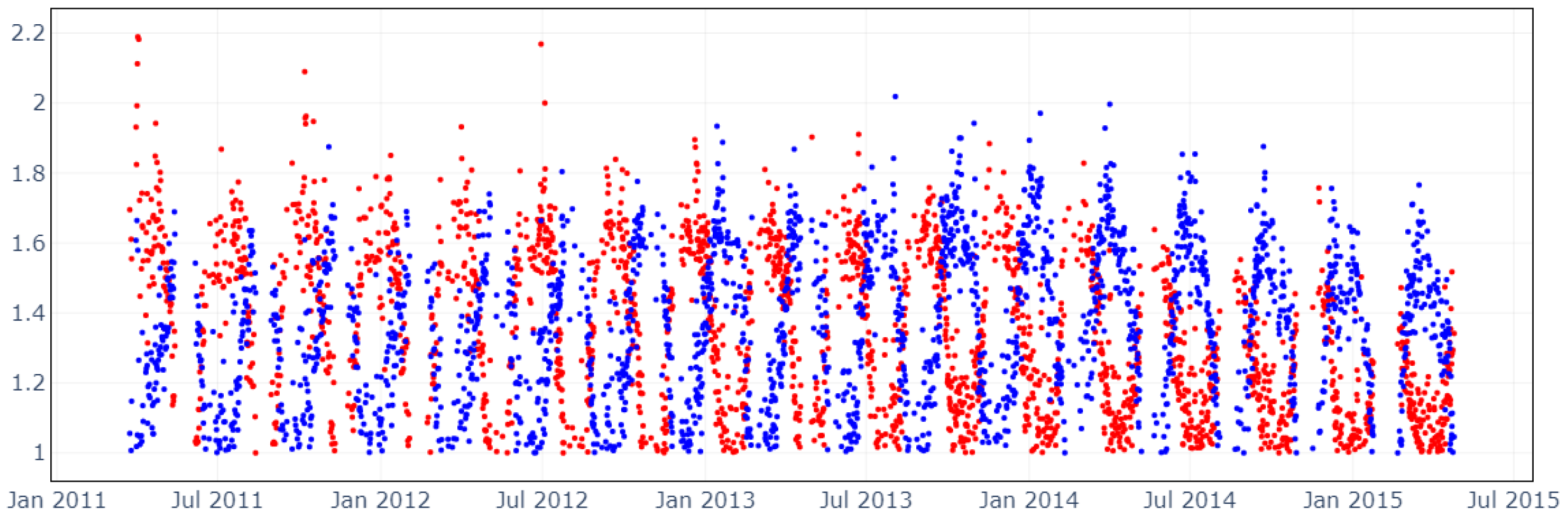
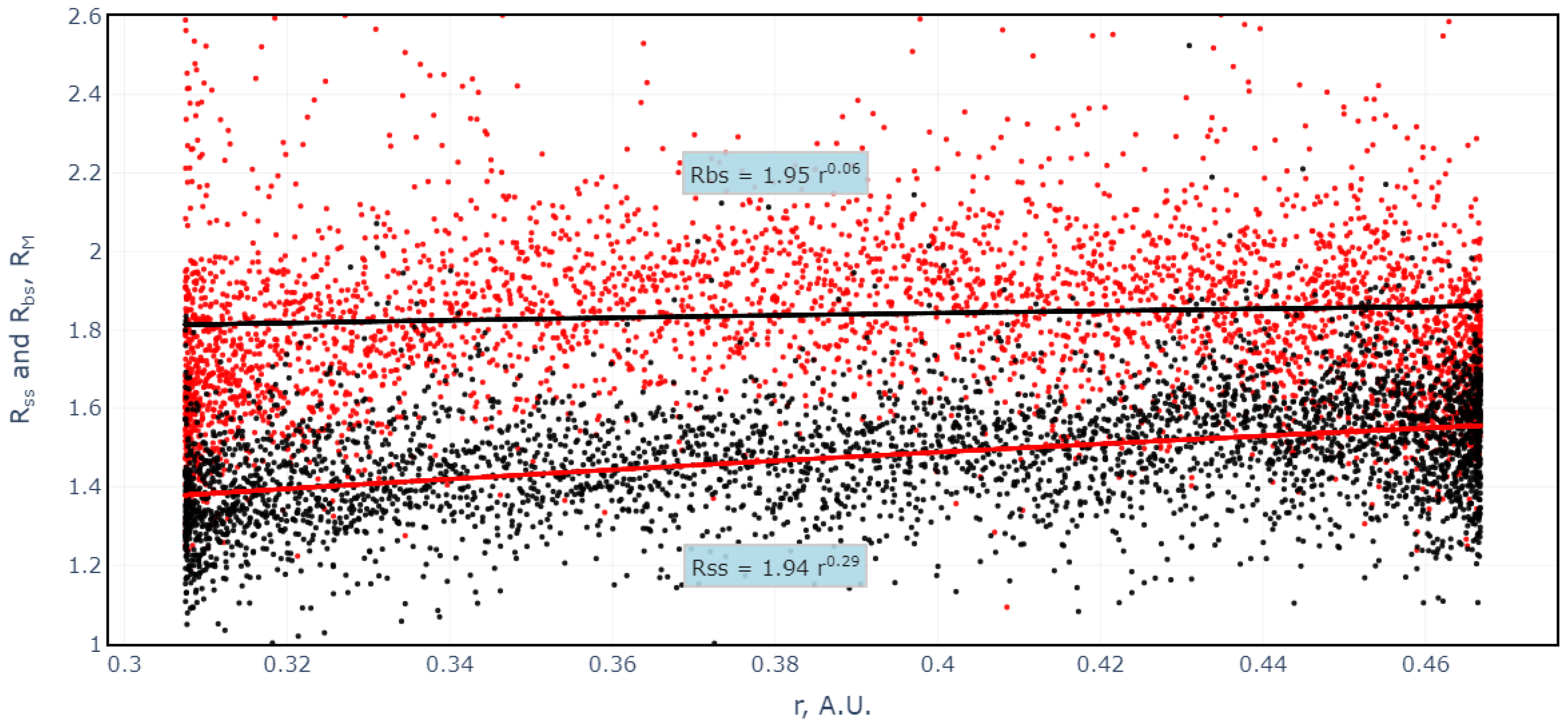
3.1. Magnetopause and Bow Shock Subsolar Distances

Figure 4 shows the bow shock and magnetopause subsolar distances, calculated using the method described above, depending on the heliocentric distance to the planet. As can be seen from the figure, both the distances to the subsolar point of the magnetopause and to the bow shock increase with increasing distance from the Sun. This effect is simply a radial plasma pressure profile which, with a fixed planetary dipole, provides visible power-law profiles.
When fitting with a dependence of the form f ( r ) = F · r b / a b , where a = r h = 0.387 AU is the average distance between Mercury and the Sun, and F = f ( r ) —the average value for one orbit of Mercury around the Sun, we obtained the following results. For the magnetopause, F = R s s = 1.48 R M , and the power coefficient b = 0.29 , which is close to the theoretically predicted value 1 / 3 , but somewhat different from it. This effect is possibly due to induction in the core of Mercury [11]. For the bow shock, F = R b s = 2.07 R M , and the power coefficient b = 0.06 , i.e., R b s decreases with increasing heliocentric distance r h , which is confirmed by other estimates [16,31], but is very slow compared to R s s . Thus, using the instantaneous surface method for all MESSENGER orbits, we obtain that the bow shock subsolar distance R b s is changing from 1.81 R M to 1.86 R M with a mean value of 1.84 R M and the magnetopause subsolar distance R s s is changing from 1.38 R M to 1.55 R M with a mean value of 1.47 R M .
A comparison of the results obtained in different papers is shown in Table 1. The power dependence of R s s on r h obtained in our work is closest to the value obtained in [11]. Ref. [11] limited their calculations to magnetopause crossings up to X > 2 R M , to minimize the effect of flaring variations. In addition, the authors limited themselves to considering orbits with an activity index of less than 33 [32], using only about 1/3 of all data. Also, the Δ R s s obtained using the paraboloid shape in our work is very close to the Δ R s s obtained using the Shue model shape [10] in [12], which suggests that, although the Shue surface better describes the cloud of all magnetopause crossing points, both approaches are valid and can be used to further study the dynamics of both the magnetopause and the magnetosheath. The ratio of aphelion and perihelion magnetopause subsolar distances is 1.12, which is close to the theoretically predicted value of 1.15.
The power dependence of R b s on r h for Mercury is considered for the first time. The obtained average bow shock subsolar distance value of 1.84 R M is smaller than that obtained in other papers, which can happen due to the fact that we considered all MESSENGER orbits and effects of the bow shock flaring on the nightside as well as extreme events were not taken in consideration. We have found that the magnetopause reaches the surface of the planet in less than 1% of cases. This is somewhat less than that obtained by [11], who have found that this case would be realized for 1.5–4% of orbits for the average Shue magnetopause shape. The mean subsolar magnetosheath thickness in this case is 0.37 R M with R b s / R s s = 1.25 , which is somewhat smaller than expected ( 1.45 R M [4,33]) due to the smaller obtained bow shock subsolar distance.

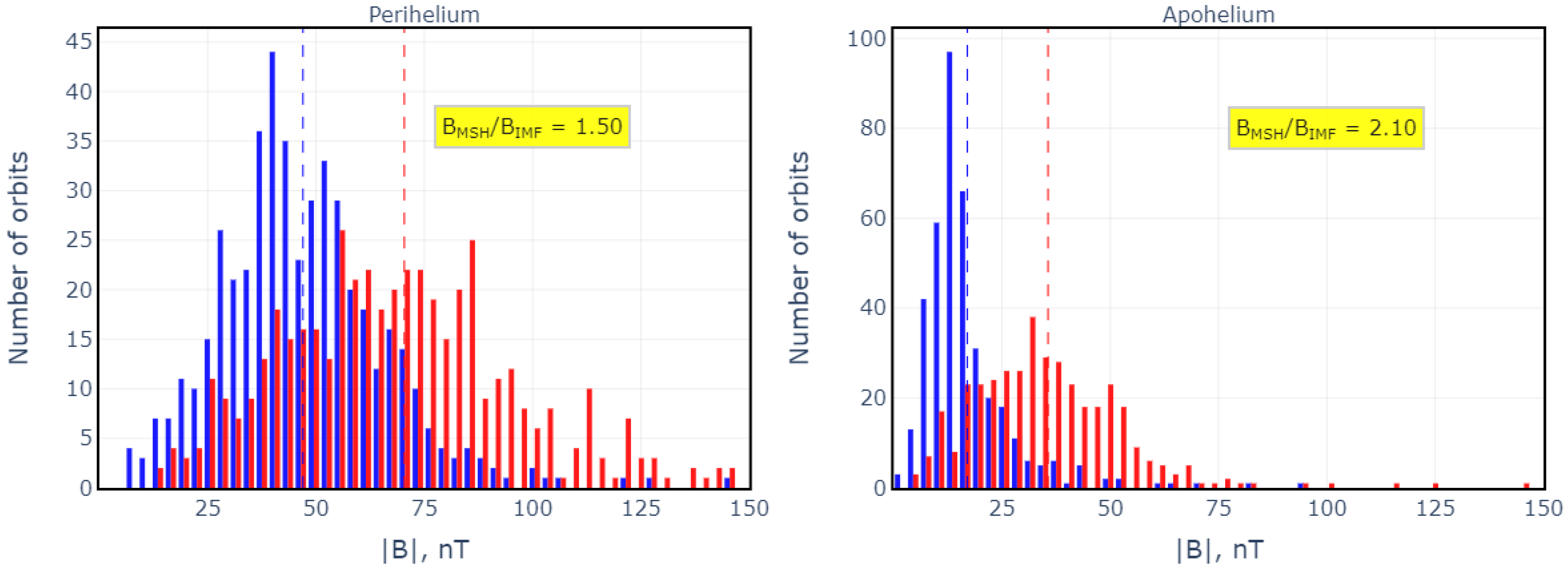
3.2. Variations of the Interplanetary Magnetic Field and the Magnetosheath Magnetic Field

The orientation and magnitude of the interplanetary magnetic field play an important role in the dynamics of planetary magnetospheres. Ref. [34] studied in detail the IMF magnitude and direction variations near Mercury, in particular the IMF clock and cone angles, and the same quantities, but in the magnetosheath region. We calculate the ratio value of the average interplanetary magnetic field magnitude to the average magnetosheath field magnitude on the dayside of the magnetosphere, as well as the average magnetosheath thickness in the subsolar point of the magnetosphere.
To determine the IMF variations, a measurement interval was chosen from the orbit, beginning with the first bow shock crossing on the descending part of the trajectory and after the last intersection of the bow shock to the end of the orbit for the ascending part from the crossings dataset [12]. These two values were then averaged to determine the IMF for a given orbit. For the magnetosheath, we chose the interval from the last bow shock crossing to the first magnetopause crossing for the descending part of the trajectory, and from the last magnetopause crossing to the first bow shock crossing on the ascending part of the trajectory from the crossings dataset [12]. Then, the magnetic field magnitudes in these intervals were averaged. To describe the orbital variations, we chose values 0.307 < r h < 0.315 for perihelion, and 0.459 < r h < 0.467 for aphelion.
The average field strength in the dayside magnetosheath is 70.38 nT and 46.98 nT of the IMF in perihelion, thus giving the ratio B m s h / B I M F = 1.50 —the degree of compression of the solar wind. The same values for aphelion are 35.63 nT and 16.99 nT, thus giving B m s h / B I M F = 2.10 (see Figure 5). One can see that the ratio B m s h / B I M F increases with the heliocentric distance increase to the planet by 1.4. We have also calculated the mean of ratios B m s h / B I M F for each orbit in perihelion and aphelion. This gave us slightly different values compared to ratio of means, 1.75 for perihelion and 2.46 for aphelion. The ratio of these values also equals 1.4. The calculated B I M F is proportional to 1 / r h 2.5 , while B m s h 1 / r h 1.7 .

4. Discussion

In this work, we have projected the MESSENGER’s bow shock and magnetopause crossing points, determined in [12], into subsolar points, and determined the subsolar distances and their variations. Observations show the existence of annual variations in the magnetopause and bow shock positions. The positions of these current systems strongly influence the magnetospheric magnetic field. The magnetopause subsolar distance R s s values vary from 1.38 R M at perihelion to 1.55 R M at aphelion. The dependence of R s s on the heliocentric distance is distinguishable and close to the predicted values. The bow shock subsolar distance R b s values vary from 1.81 R M at perihelion to 1.86 R M at aphelion. The dependence of R b s on the heliocentric distance is difficult to distinguish. The moving average of R b s in Figure 4 is almost parallel to the horizontal axis.
We considered the magnetic field variations in the interplanetary space and in the magnetosheath of the Mercury magnetosphere for each MESSENGER orbit. These quantities also vary with the heliocentric distance from the planet. On average, the magnetic field during the transition from interplanetary space to the dayside magnetosheath region increases by a factor of 1.50 in Mercury’s orbit perihelion to 2.10 in aphelion.
It should be noted that, in addition to the main factor, which leads to variations in solar wind pressure depending on the heliocentric distance, there are also other effects that are not considered in this paper, but which can play a certain role: the effect of erosion of the daytime magnetopause, which leads to a subsolar distance decrease under southward IMF [17]; the radial IMF direction influence [15,35]; and the induced field from the conductive core influence [11,36].

5. Conclusions

To determine the distance to the subsolar point of the magnetopause and the bow shock, we recalculated the coordinates of the point where MESSENGER crossed the magnetopause and the bow shock using the average shapes of these surfaces. We approximated both surfaces as a paraboloid of revolution. Since the solar wind pressure at the dayside magnetopause varied due to the strong eccentricity of Mercury’s orbit around the Sun, we confirmed a dependence of the magnetosphere on dynamic solar wind pressure. The power index for that dependence, which was found to be 0.29, is in agreement with the results previously obtained with different methods [4,11]. Comparing to [12], we also calculated the distance to the subsolar point of the bow shock as a function of the dynamic pressure of the solar wind, and found that this distance is almost independent of pressure. Additionally, we calculated the degree of “compression” of the magnetic field at the front of the bow shock. Downstream from the front, the magnetic field was found to be, on average, twice as strong as the undisturbed field upstream of the bow shock.

Author Contributions

Conceptualization, D.N. and I.A.; methodology, D.N. and A.L.; software, D.N.; validation, A.L. and I.A.; formal analysis, D.N. and A.L.; investigation, D.N. and A.L.; resources, D.N. and A.L.; data curation, D.N. and A.L.; writing—original draft preparation, A.L.; writing—review and editing, A.L. and I.A.; visualization, A.L. and D.N.; supervision, I.A.; project administration, A.L.; funding acquisition, I.A. All authors have read and agreed to the published version of the manuscript.

Funding

This research was funded by RFBR grant number 21-52-12025.

Data Availability Statement

Publicly available datasets were analyzed in this study. These data can be found here: https://doi.org/10.5683/SP2/1U6FEO, access granted on 1 September 2023.

Conflicts of Interest

The authors declare no conflicts of interest. The funders had no role in the design of the study; in the collection, analyses, or interpretation of data; in the writing of the manuscript; or in the decision to publish the results.

Abbreviation

The following abbreviation is used in this manuscript:
IMFInterplanetary Magnetic Field

References

  1. Alexeev, I.I.; Belenkaya, E.S.; Bobrovnikov, S.Y.; Slavin, J.A.; Sarantos, M. Paraboloid model of Mercury’s magnetosphere. J. Geophys. Res. Space Phys. 2008, 113, A12210. [Google Scholar] [CrossRef]
  2. Alexeev, I.I.; Belenkaya, E.S.; Slavin, J.A.; Korth, H.; Anderson, B.J.; Baker, D.N.; Boardsen, S.A.; Johnson, C.L.; Purucker, M.E.; Sarantos, M.; et al. Mercury’s magnetospheric magnetic field after the first two MESSENGER flybys. Icarus 2010, 209, 23–39. [Google Scholar] [CrossRef]
  3. Anderson, B.J.; Johnson, C.L.; Korth, H.; Winslow, R.M.; Borovsky, J.E.; Purucker, M.E.; Slavin, J.A.; Solomon, S.C.; Zuber, M.T.; McNutt, R.L., Jr. Low-degree structure in Mercury’s planetary magnetic field. J. Geophys. Res. Planets 2012, 117. [Google Scholar] [CrossRef]
  4. Winslow, R.M.; Anderson, B.J.; Johnson, C.L.; Slavin, J.A.; Korth, H.; Purucker, M.E.; Baker, D.N.; Solomon, S.C. Mercury’s magnetopause and bow shock from MESSENGER Magnetometer observations. J. Geophys. Res. Space Phys. 2013, 118, 2213–2227. [Google Scholar] [CrossRef]
  5. Slavin, J.A.; DiBraccio, G.A.; Gershman, D.J.; Imber, S.M.; Poh, G.K.; Raines, J.M.; Zurbuchen, T.H.; Jia, X.; Baker, D.N.; Glassmeier, K.H.; et al. MESSENGER observations of Mercury’s dayside magnetosphere under extreme solar wind conditions. J. Geophys. Res. Space Phys. 2014, 119, 8087–8116. [Google Scholar] [CrossRef]
  6. Slavin, J.A.; Middleton, H.R.; Raines, J.M.; Jia, X.; Zhong, J.; Sun, W.J.; Livi, S.; Imber, S.M.; Poh, G.K.; Akhavan-Tafti, M.; et al. MESSENGER Observations of Disappearing Dayside Magnetosphere Events at Mercury. J. Geophys. Res. Space Phys. 2019, 124, 6613–6635. [Google Scholar] [CrossRef]
  7. Philpott, L.C.; Johnson, C.L.; Winslow, R.M.; Anderson, B.J.; Korth, H.; Purucker, M.E.; Solomon, S.C. Constraints on the secular variation of Mercury’s magnetic field from the combined analysis of MESSENGER and Mariner 10 data. Geophys. Res. Lett. 2014, 41, 6627–6634. [Google Scholar] [CrossRef]
  8. Siscoe, G.; Christopher, L. Variations in the solar wind stand-off distance at Mercury. Geophys. Res. Lett. 1975, 2, 158–160. [Google Scholar] [CrossRef]
  9. Russell, C.T. On the relative locations of the bow shocks of the terrestrial planets. Geophys. Res. Lett. 1977, 4, 387–390. [Google Scholar] [CrossRef]
  10. Shue, J.H.; Chao, J.K.; Fu, H.C.; Russell, C.T.; Song, P.; Khurana, K.K.; Singer, H.J. A new functional form to study the solar wind control of the magnetopause size and shape. J. Geophys. Res. Space Phys. 1997, 102, 9497–9511. [Google Scholar] [CrossRef]
  11. Johnson, C.L.; Philpott, L.C.; Anderson, B.J.; Korth, H.; Hauck II, S.A.; Heyner, D.; Phillips, R.J.; Winslow, R.M.; Solomon, S.C. MESSENGER observations of induced magnetic fields in Mercury’s core. Geophys. Res. Lett. 2016, 43, 2436–2444. [Google Scholar] [CrossRef]
  12. Philpott, L.C.; Johnson, C.L.; Anderson, B.J.; Winslow, R.M. The Shape of Mercury’s Magnetopause: The Picture From MESSENGER Magnetometer Observations and Future Prospects for BepiColombo. J. Geophys. Res. Space Phys. 2020, 125, e2019JA027544. [Google Scholar] [CrossRef]
  13. Zhong, J.; Wan, W.X.; Slavin, J.A.; Wei, Y.; Lin, R.L.; Chai, L.H.; Raines, J.M.; Rong, Z.J.; Han, X.H. Mercury’s three-dimensional asymmetric magnetopause. J. Geophys. Res. Space Phys. 2015, 120, 7658–7671. [Google Scholar] [CrossRef]
  14. Zhong, J.; Wan, W.X.; Wei, Y.; Slavin, J.A.; Raines, J.M.; Rong, Z.J.; Chai, L.H.; Han, X.H. Compressibility of Mercury’s dayside magnetosphere. Geophys. Res. Lett. 2015, 42, 10135–10139. [Google Scholar] [CrossRef]
  15. Zhong, J.H.; Shue, J.H.; Wei, Y.; Slavin, J.A.; Zhang, H.; Rong, Z.J.; Chai, L.H.; Wan, W.X. Effects of Orbital Eccentricity and IMF Cone Angle on the Dimensions of Mercury’s Magnetosphere. Astrophys. J. 2020, 892, 2. [Google Scholar] [CrossRef]
  16. He, P.; Xu, X.; Yu, H.; Wang, X.; Wang, M.; Chang, Q.; Zhou, Z.; Luo, L.; Li, H. The Mercury’s Bow-shock Models Near Perihelion and Aphelion. Astron. J. 2022, 164, 260. [Google Scholar] [CrossRef]
  17. Slavin, J.A.; Holzer, R.E. The effect of erosion on the solar wind stand-off distance at Mercury. J. Geophys. Res. Space Phys. 1979, 84, 2076–2082. [Google Scholar] [CrossRef]
  18. Boardsen, S.A.; Sundberg, T.; Slavin, J.A.; Anderson, B.J.; Korth, H.; Solomon, S.C.; Blomberg, L.G. Observations of Kelvin-Helmholtz waves along the dusk-side boundary of Mercury’s magnetosphere during MESSENGER’s third flyby. Geophys. Res. Lett. 2010, 37, L12101. [Google Scholar] [CrossRef]
  19. Slavin, J.A.; Acuña, M.H.; Anderson, B.J.; Baker, D.N.; Benna, M.; Gloeckler, G.; Gold, R.E.; Ho, G.C.; Killen, R.M.; Korth, H.; et al. Mercury’s Magnetosphere After MESSENGER’s First Flyby. Science 2008, 321, 85–89. [Google Scholar] [CrossRef]
  20. Belenkaya, E.; Pensionerov, I. What Density of Magnetosheath Sodium Ions Can Provide the Observed Decrease in the Magnetic Field of the “Double Magnetopause” during the First MESSENGER Flyby? Symmetry 2021, 13, 1168. [Google Scholar] [CrossRef]
  21. DiBraccio, G.A.; Slavin, J.A.; Boardsen, S.A.; Anderson, B.J.; Korth, H.; Zurbuchen, T.H.; Raines, J.M.; Baker, D.N.; McNutt, R.L., Jr.; Solomon, S.C. MESSENGER observations of magnetopause structure and dynamics at Mercury. J. Geophys. Res. Space Phys. 2013, 118, 997–1008. [Google Scholar] [CrossRef]
  22. Zhong, J.; Lee, L.C.; Slavin, J.A.; Zhang, H.; Wei, Y. MESSENGER Observations of Reconnection in Mercury’s Magnetotail Under Strong IMF Forcing. J. Geophys. Res. Space Phys. 2023, 128, e2022JA031134. [Google Scholar] [CrossRef]
  23. Veselovsky, I.S.; Dmitriev, A.V.; Suvorova, A.V.; Tarsina, M.V. Solar wind variation with the cycle. J. Astrophys. Astron. 2000, 21, 423–429. [Google Scholar] [CrossRef]
  24. Chapman, J.F.; Cairns, I.H. Three-dimensional modeling of Earth’s bow shock: Shock shape as a function of Alfvén Mach number. J. Geophys. Res. Space Phys. 2003, 108, 1174. [Google Scholar] [CrossRef]
  25. Slavin, J.A.; Anderson, B.J.; Zurbuchen, T.H.; Baker, D.N.; Krimigis, S.M.; Acuña, M.H.; Benna, M.; Boardsen, S.A.; Gloeckler, G.; Gold, R.E.; et al. MESSENGER observations of Mercury’s magnetosphere during northward IMF. Geophys. Res. Lett. 2009, 36, L02101. [Google Scholar] [CrossRef]
  26. Belenkaya, E.; Bobrovnikov, S.; Alexeev, I.; Kalegaev, V.; Cowley, S. A model of Jupiter’s magnetospheric magnetic field with variable magnetopause flaring. Planet. Space Sci. 2005, 53, 863–872. [Google Scholar] [CrossRef]
  27. Johnson, C.L.; Purucker, M.E.; Korth, H.; Anderson, B.J.; Winslow, R.M.; Al Asad, M.M.H.; Slavin, J.A.; Alexeev, I.I.; Phillips, R.J.; Zuber, M.T.; et al. MESSENGER observations of Mercury’s magnetic field structure. J. Geophys. Res. Planets 2012, 117, E00L14. [Google Scholar] [CrossRef]
  28. Heyner, D.; Nabert, C.; Liebert, E.; Glassmeier, K.H. Concerning reconnection-induction balance at the magnetopause of Mercury. J. Geophys. Res. Space Phys. 2016, 121, 2935–2961. [Google Scholar] [CrossRef]
  29. Winslow, R.M.; Philpott, L.; Paty, C.S.; Lugaz, N.; Schwadron, N.A.; Johnson, C.L.; Korth, H. Statistical study of ICME effects on Mercury’s magnetospheric boundaries and northern cusp region from MESSENGER. J. Geophys. Res. Space Phys. 2017, 122, 4960–4975. [Google Scholar] [CrossRef]
  30. Kobel, E.; Flückiger, E.O. A model of the steady state magnetic field in the magnetosheath. J. Geophys. Res. Space Phys. 1994, 99, 23617–23622. [Google Scholar] [CrossRef]
  31. Heyner, D.; Auster, H.U.; Fornaçon, K.H.; Carr, C.; Richter, I.; Mieth, J.Z.D.; Kolhey, P.; Exner, W.; Motschmann, U.; Baumjohann, W.; et al. The BepiColombo Planetary Magnetometer MPO-MAG: What Can We Learn from the Hermean Magnetic Field? Space Sci. Rev. 2021, 217, 52. [Google Scholar] [CrossRef]
  32. Anderson, B.J.; Johnson, C.L.; Korth, H. A magnetic disturbance index for Mercury’s magnetic field derived from MESSENGER Magnetometer data. Geochem. Geophys. Geosystems 2013, 14, 3875–3886. [Google Scholar] [CrossRef]
  33. Alexeev, I.; Parunakian, D.; Dyadechkin, S.; Belenkaya, E.; Khodachenko, M.; Kallio, E.; Alho, M. Calculation of the Initial Magnetic Field for Mercury’s Magnetosphere Hybrid Model. Cosm. Res. 2018, 56, 108–114. [Google Scholar] [CrossRef]
  34. James, M.K.; Imber, S.M.; Bunce, E.J.; Yeoman, T.K.; Lockwood, M.; Owens, M.J.; Slavin, J.A. Interplanetary magnetic field properties and variability near Mercury’s orbit. J. Geophys. Res. Space Phys. 2017, 122, 7907–7924. [Google Scholar] [CrossRef]
  35. Belenkaya, E.S. Reconnection modes for near-radial interplanetary magnetic field. J. Geophys. Res. Space Phys. 1998, 103, 26487–26494. [Google Scholar] [CrossRef]
  36. Wardinski, I.; Langlais, B.; Thébault, E. Correlated Time-Varying Magnetic Fields and the Core Size of Mercury. J. Geophys. Res. Planets 2019, 124, 2178–2197. [Google Scholar] [CrossRef]
Figure 1. The average position of the bow shock crossings by MESSENGER for all orbits. The color of crossings depends on the distance to the Sun (red—for orbits at aphelion, blue—for orbits at perihelion with white at the middle). Crossing points are fitted by paraboloid (light green curve) and hyperboloid [25] (yellow curve). Mercury is shown shifted southward to account for dipole offset in the northern hemisphere.
Universe 10 00040 g001
Figure 2. The average position of the magnetopause crossings by MESSENGER for all orbits. The color of crossings depends on the distance to the Sun (red—for orbits at aphelion, blue—for orbits at perihelion with white at the middle). Crossing points are fitted by paraboloid (light green curve) and Shue [10] shapes (yellow curve). Mercury is shown to be shifted southward to account for dipole offset in the northern hemisphere.
Universe 10 00040 g002
Figure 3. Magnetopause standoff distance values ( R s s ), obtained for descending (red) and ascending (blue) parts of MESSENGER orbit around Mercury for all MESSENGER orbits. Clear bimodal distribution, related to the “observer” effect (described below in the text), is seen.
Universe 10 00040 g003
Figure 4. Distribution of the magnetopause and the bow shock subsolar distances depending on the heliocentric distance to Mercury, calculated from the coordinates of the crossing points of magnetopause (red dots) and bow shock (black dots). The subsolar distance is given along the vertical axis in the Mercury radii. The straight lines show the fit of the magnetopause (red line) and bow shock (black line) positions over the entire set of points. The horizontal axis indicates the heliocentric distance to Mercury in AU.
Universe 10 00040 g004
Figure 5. Distributions histogram of number of orbits by the IMF strength (blue) and the same distribution for magnetosheath magnetic field strength (red) for orbits in perihelion (left) and aphelion (right).
Universe 10 00040 g005
Table 1. Comparison of R s s (magnetopause) and R b s (bow shock) heliocentric dependencies.
Paper R ss , R M Δ R ss , R M R ss Power Index R bs , R M Δ R bs , R M R bs Power Index
Siscoe 1975 [8]1.91.7–2.0- --
Russell 1977 [9]1.3--1.9--
Winslow 2013 [4]1.451.35–1.550.301.961.89–2.29-
Zhong 2015 [14]1.511.38–1.650.42---
Johnson 2016 [11]--0.29---
Zhong 2020 [15]-1.43–1.600.22---
Philpott 2020 [12]1.461.40–1.54----
He 2022 [16]----1.92–2.10-
Current paper1.481.38–1.550.291.841.81–1.860.06
Disclaimer/Publisher’s Note: The statements, opinions and data contained in all publications are solely those of the individual author(s) and contributor(s) and not of MDPI and/or the editor(s). MDPI and/or the editor(s) disclaim responsibility for any injury to people or property resulting from any ideas, methods, instructions or products referred to in the content.

