
Automated Cancer Diagnostics via Analysis of Optical and Chemical Images by Deep and Shallow Learning

 , , , , and
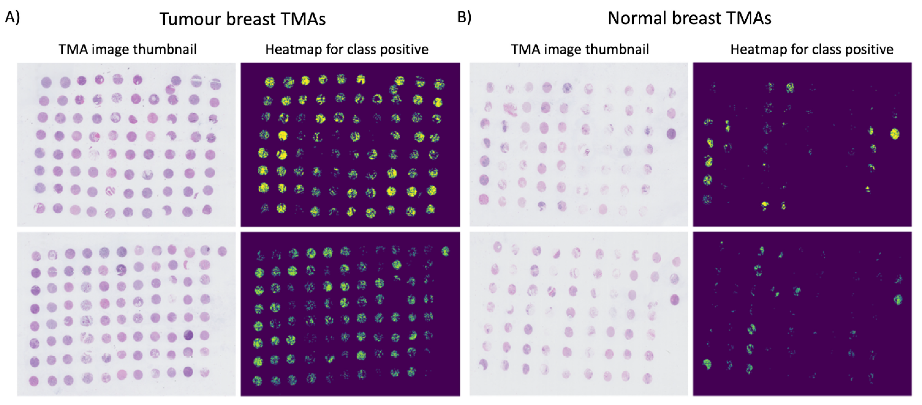
Abstract
:1. Introduction
2. Results & Discussion
2.1. Optical Imaging-Based Deep Learning Approach
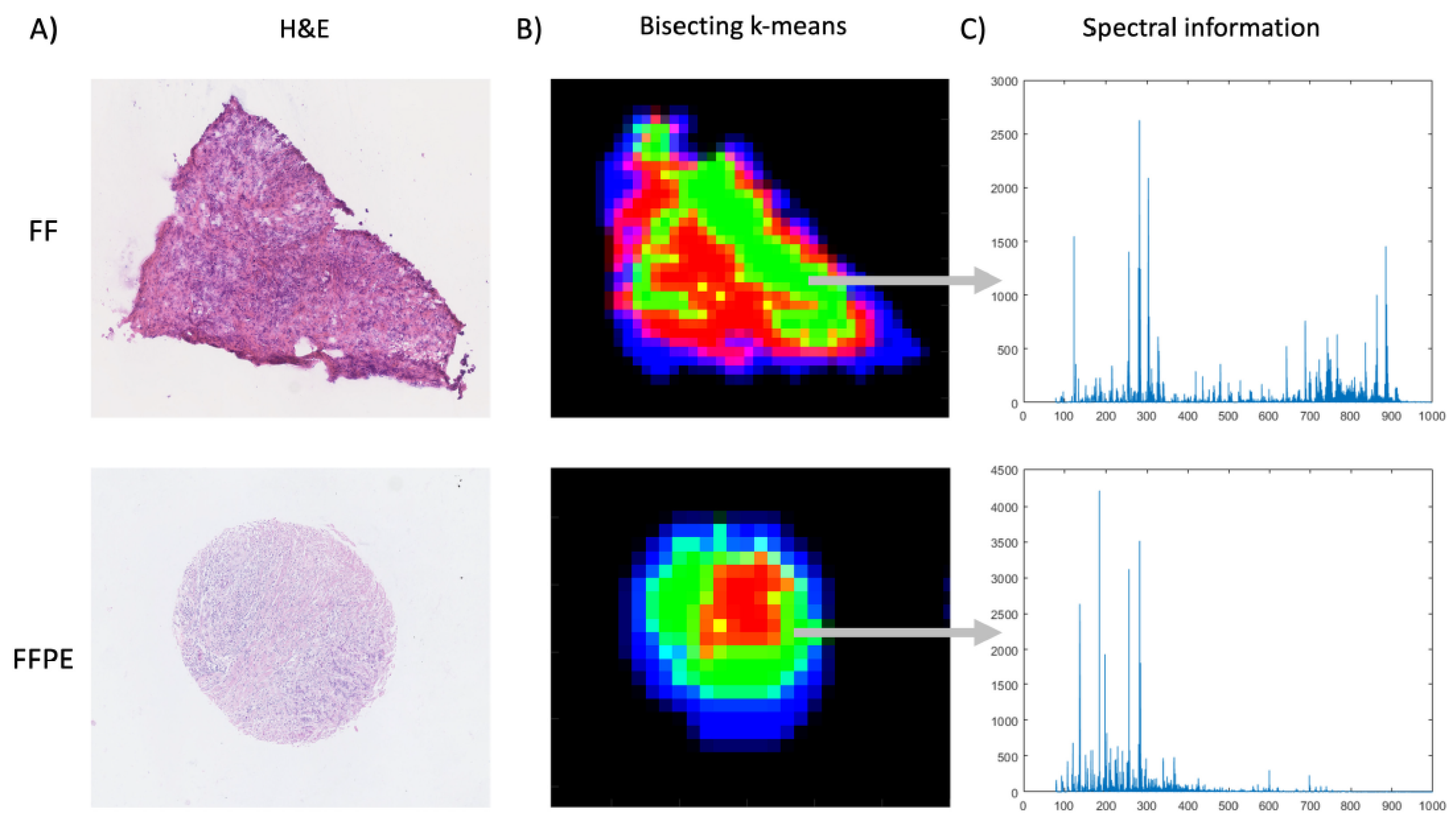
2.2. DESI-MSI-Based Shallow Learning Approach
3. Materials and Methods
3.1. Materials
3.2. Deep Learning
3.2.1. Optical Imaging
3.2.2. Training Data
3.2.3. Algorithm
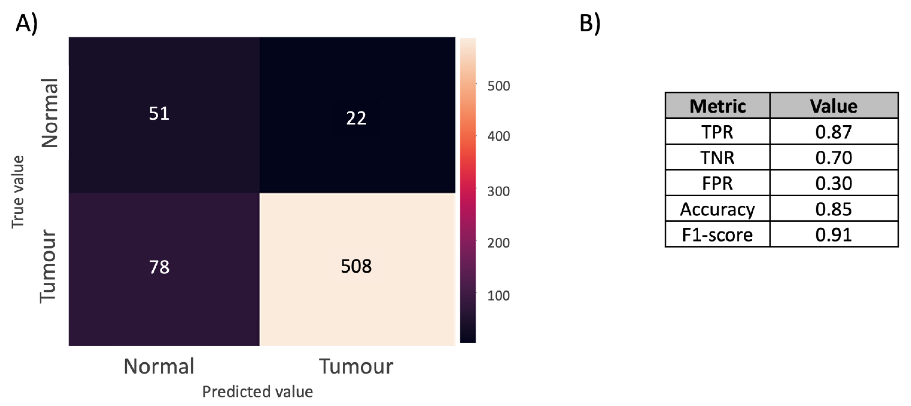
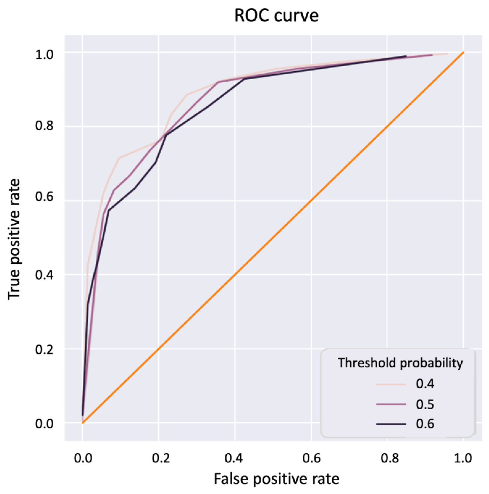
3.2.4. Model Performance Evaluation
3.3. Shallow learning
3.3.1. DESI-MSI Analysis
3.3.2. MSI Data Pre-Processing
3.3.3. Supervised Shallow Learning & Statistical Analysis
4. Conclusions
Supplementary Materials
Author Contributions
Funding
Institutional Review Board Statement
Informed Consent Statement
Data Availability Statement
Conflicts of Interest
Abbreviations
| AUC | Area under the curve |
| CAD | Computer-assisted diagnostics |
| CNN | Convolutional neural network |
| DESI | Desorption electrospray ionisation |
| DL | Deep learning |
| FF | Fresh frozen |
| FFPE | Formalin-fixed and paraffin-embedded |
| FPR | False positive rate |
| HDF5 | Hierarchical data format version 5 |
| H&E | Haematoxylin and eosin |
| IHC | Immunohistochemistry |
| LR | Logistic regression |
| MALDI | Matrix-assisted desorption/ionisation |
| MIL | Multiple instance learning |
| MS | Mass spectrometry |
| MSI | Mass spectrometry imaging |
| PCA | Principal component analysis |
| ROC | Receiver operating characteristic |
| ROI | Region-of-interest |
| SNR | Signal-to-noise ratio |
| TNR | True negative rate |
| TMA | Tissue microarray |
| TPR | True positive rate |
| WSI | Whole-slide image |
References
- He, L.; Long, L.R.; Antani, S.; Thoma, G.R. Histology image analysis for carcinoma detection and grading. Comput. Methods Programs Biomed. 2012, 107, 538–556. [Google Scholar] [CrossRef] [PubMed] [Green Version]
- Donczo, B.; Guttman, A. Biomedical analysis of formalin-fixed, paraffin-embedded tissue samples: The Holy Grail for molecular diagnostics. J. Pharm. Biomed. Anal. 2018, 155, 125–134. [Google Scholar] [CrossRef] [PubMed] [Green Version]
- Gaffney, E.F.; Riegman, P.H.; Grizzle, W.E.; Watson, P.H. Factors that drive the increasing use of FFPE tissue in basic and translational cancer research. Biotech. Histochem. 2018, 93, 373–386. [Google Scholar] [CrossRef] [PubMed] [Green Version]
- Arima, K.; Lau, M.C.; Zhao, M.; Haruki, K.; Kosumi, K.; Mima, K.; Gu, M.; Väyrynen, J.P.; Twombly, T.S.; Baba, Y.; et al. Metabolic profiling of formalin-fixed paraffin-embedded tissues discriminates normal colon from colorectal cancer. Mol. Cancer Res. 2020, 18, 883–890. [Google Scholar] [CrossRef] [PubMed] [Green Version]
- Buck, A.; Ly, A.; Balluff, B.; Sun, N.; Gorzolka, K.; Feuchtinger, A.; Janssen, K.P.; Kuppen, P.J.; Van De Velde, C.J.; Weirich, G.; et al. High-resolution MALDI-FT-ICR MS imaging for the analysis of metabolites from formalin-fixed, paraffin-embedded clinical tissue samples. J. Pathol. 2015, 237, 123–132. [Google Scholar] [CrossRef] [PubMed] [Green Version]
- Schwamborn, K. The Importance of Histology and Pathology in Mass Spectrometry Imaging, 1st ed.; Elsevier Inc.: Amsterdam, The Netherlands, 2017; Volume 134, pp. 1–26. [Google Scholar] [CrossRef]
- Warth, A.; Stenzinger, A.; Andrulis, M.; Schlake, W.; Kempny, G.; Schirmacher, P.; Weichert, W. Individualized medicine and demographic change as determining workload factors in pathology: Quo vadis? Virchows Arch. 2016, 468, 101–108. [Google Scholar] [CrossRef]
- Cui, M.; Zhang, D.Y. Artificial intelligence and computational pathology. Lab. Investig. 2021, 101, 412–422. [Google Scholar] [CrossRef]
- Balog, J.; Szaniszlo, T.; Schaefer, K.C.; Denes, J.; Lopata, A.; Godorhazy, L.; Szalay, D.; Balogh, L.; Sasi-Szabo, L.; Toth, M.; et al. Identification of biological tissues by rapid evaporative ionization mass spectrometry. Anal. Chem. 2010, 82, 7343–7350. [Google Scholar] [CrossRef]
- Ogrinc, N.; Caux, P.D.; Robin, Y.M.; Bouchaert, E.; Fatou, B.; Ziskind, M.; Focsa, C.; Bertin, D.; Tierny, D.; Takats, Z.; et al. Direct Water-Assisted Laser Desorption/Ionization Mass Spectrometry Lipidomic Analysis and Classification of Formalin-Fixed Paraffin-Embedded Sarcoma Tissues without Dewaxing. Clin. Chem. 2021, 67, 1513–1523. [Google Scholar] [CrossRef]
- Campanella, G.; Hanna, M.G.; Geneslaw, L.; Miraflor, A.; Werneck Krauss Silva, V.; Busam, K.J.; Brogi, E.; Reuter, V.E.; Klimstra, D.S.; Fuchs, T.J. Clinical-grade computational pathology using weakly supervised deep learning on whole slide images. Nat. Med. 2019, 25, 1301–1309. [Google Scholar] [CrossRef]
- Indica Labs Inc. Halo AI. 2022. Available online: https://indicalab.com/halo-ai/ (accessed on 19 April 2022).
- Visiopharm. 2022. Available online: https://visiopharm.com (accessed on 19 April 2022).
- Cruz-Roa, A.; Gilmore, H.; Basavanhally, A.; Feldman, M.; Ganesan, S.; Shih, N.N.; Tomaszewski, J.; González, F.A.; Madabhushi, A. Accurate and reproducible invasive breast cancer detection in whole-slide images: A Deep Learning approach for quantifying tumor extent. Sci. Rep. 2017, 7, 46450. [Google Scholar] [CrossRef] [PubMed] [Green Version]
- Castaing, R.; Slodzian, G. Optique Corpusculaire—Premiers Essais De Microanalyse Par Emission Ionique Secondaire. CR Hebd. Acad. Sci. 1962, 395. [Google Scholar]
- Porta Siegel, T.; Hamm, G.; Bunch, J.; Cappell, J.; Fletcher, J.S.; Schwamborn, K. Mass Spectrometry Imaging and Integration with Other Imaging Modalities for Greater Molecular Understanding of Biological Tissues. Mol. Imaging Biol. 2018, 20, 888–901. [Google Scholar] [CrossRef] [PubMed] [Green Version]
- Tákats, Z.; Wiseman, J.M.; Gologan, B.; Cooks, R.G. Mass spectrometry sampling under ambient conditions with desorption electrospray ionization. Science 2004, 306, 471–473. [Google Scholar] [CrossRef] [Green Version]
- Takats, Z.; Strittmatter, N.; McKenzie, J.S. Ambient Mass Spectrometry in Cancer Research, 1st ed.; Elsevier Inc.: Amsterdam, The Netherlands, 2017; Volume 134, pp. 231–256. [Google Scholar] [CrossRef]
- Abbassi-Ghadi, N.; Veselkov, K.; Kumar, S.; Huang, J.; Jones, E.; Strittmatter, N.; Kudo, H.; Goldin, R.; Takáts, Z.; Hanna, G.B. Discrimination of lymph node metastases using desorption electrospray ionisation-mass spectrometry imaging. Chem. Commun. 2014, 50, 3661–3664. [Google Scholar] [CrossRef]
- Wiseman, J.M.; Ifa, D.R.; Venter, A.; Cooks, R.G. Ambient molecular imaging by desorption electrospray ionization mass spectrometry. Nat. Protoc. 2008, 3, 517–524. [Google Scholar] [CrossRef]
- Buck, A.; Heijs, B.; Beine, B.; Schepers, J.; Cassese, A.; Heeren, R.M.; McDonnell, L.A.; Henkel, C.; Walch, A.; Balluff, B. Round robin study of formalin-fixed paraffin-embedded tissues in mass spectrometry imaging. Anal. Bioanal. Chem. 2018, 410, 5969–5980. [Google Scholar] [CrossRef] [Green Version]
- Dória, M.L.; McKenzie, J.S.; Mroz, A.; Phelps, D.L.; Speller, A.; Rosini, F.; Strittmatter, N.; Golf, O.; Veselkov, K.; Brown, R.; et al. Epithelial ovarian carcinoma diagnosis by desorption electrospray ionization mass spectrometry imaging. Sci. Rep. 2016, 6, 39219. [Google Scholar] [CrossRef] [Green Version]
- Guenther, S.; Muirhead, L.J.; Speller, A.V.; Golf, O.; Strittmatter, N.; Ramakrishnan, R.; Goldin, R.D.; Jones, E.; Veselkov, K.; Nicholson, J.; et al. Spatially resolved metabolic phenotyping of breast cancer by desorption electrospray ionization mass spectrometry. Cancer Res. 2015, 75, 1828–1837. [Google Scholar] [CrossRef] [Green Version]
- Sans, M.; Gharpure, K.; Tibshirani, R.; Zhang, J.; Liang, L.; Liu, J.; Young, J.H.; Dood, R.L.; Sood, A.K.; Eberlin, L.S. Metabolic markers and statistical prediction of serous ovarian cancer aggressiveness by ambient ionization mass spectrometry imaging. Cancer Res. 2017, 77, 2903–2913. [Google Scholar] [CrossRef] [Green Version]
- Porcari, A.M.; Zhang, J.; Garza, K.Y.; Rodrigues-Peres, R.M.; Lin, J.Q.; Young, J.H.; Tibshirani, R.; Nagi, C.; Paiva, G.R.; Carter, S.A.; et al. Multicenter Study Using Desorption-Electrospray-Ionization-Mass-Spectrometry Imaging for Breast-Cancer Diagnosis. Anal. Chem. 2018, 90, 11324–11332. [Google Scholar] [CrossRef] [PubMed]
- Santoro, A.L.; Drummond, R.D.; Silva, I.T.; Ferreira, S.S.; Juliano, L.; Vendramini, P.H.; da Costa Lemos, M.B.; Eberlin, M.N.; Andrade, V.P. In situ Desi-MSI lipidomic profiles of breast cancer molecular subtypes and precursor lesions. Cancer Res. 2020, 80, 1246–1257. [Google Scholar] [CrossRef] [PubMed] [Green Version]
- Veselkov, K.A.; Mirnezami, R.; Strittmatter, N.; Goldin, R.D.; Kinross, J.; Speller, A.V.; Abramov, T.; Jones, E.A.; Darzi, A.; Holmes, E.; et al. Chemo-informatic strategy for imaging mass spectrometry-based hyperspectral profiling of lipid signatures in colorectal cancer. Proc. Natl. Acad. Sci. USA 2014, 111, 1216–1221. [Google Scholar] [CrossRef] [PubMed] [Green Version]
- Tsymbal, A. The Problem of Concept Drift: Definitions and Related Work; Technical Report; Trinity College Dublin: Dublin, Ireland, 2004. [Google Scholar]
- Dhanachandra, N.; Manglem, K.; Chanu, Y.J. Image Segmentation Using K-means Clustering Algorithm and Subtractive Clustering Algorithm. Procedia Comput. Sci. 2015, 54, 764–771. [Google Scholar] [CrossRef] [Green Version]
- Wojakowska, A.; Marczak, Ł.; Jelonek, K.; Polanski, K.; Widlak, P.; Pietrowska, M. An optimized method of metabolite extraction from formalin-fixed paraffin-embedded tissue for GC/MS analysis. PLoS ONE 2015, 10, e0136902. [Google Scholar] [CrossRef] [Green Version]
- Hughes, C.; Gaunt, L.; Brown, M.; Clarke, N.W.; Gardner, P. Assessment of paraffin removal from prostate FFPE sections using transmission mode FTIR-FPA imaging. Anal. Methods 2014, 6, 1028–1035. [Google Scholar] [CrossRef] [Green Version]
- Casadonte, R.; Kriegsmann, M.; Zweynert, F.; Friedrich, K.; Bretton, G.; Otto, M.; Deininger, S.O.; Paape, R.; Belau, E.; Suckau, D.; et al. Imaging mass spectrometry to discriminate breast from pancreatic cancer metastasis in formalin-fixed paraffin-embedded tissues. Proteomics 2014, 14, 956–964. [Google Scholar] [CrossRef]
- Ly, A.; Buck, A.; Balluff, B.; Sun, N.; Gorzolka, K.; Feuchtinger, A.; Janssen, K.P.; Kuppen, P.J.; Van De Velde, C.J.; Weirich, G.; et al. High-mass-resolution MALDI mass spectrometry imaging of metabolites from formalin-fixed paraffin-embedded tissue. Nat. Protoc. 2016, 11, 1428–1443. [Google Scholar] [CrossRef]
- Chughtai, K.; Heeren, R.M. Mass spectrometric imaging for biomedical tissue analysis. Chem. Rev. 2010, 110, 3237–3277. [Google Scholar] [CrossRef] [Green Version]
- Norris, J.L.; Caprioli, R.M. Analysis of tissue specimens by matrix-assisted laser desorption/ionization imaging mass spectrometry in biological and clinical research. Chem. Rev. 2013, 113, 2309–2342. [Google Scholar] [CrossRef] [Green Version]
- Taylor, A.J.; Dexter, A.; Bunch, J. Exploring Ion Suppression in Mass Spectrometry Imaging of a Heterogeneous Tissue. Anal. Chem. 2018, 90, 5637–5645. [Google Scholar] [CrossRef] [PubMed]
- Isberg, O.G.; Xiang, Y.; Bodvarsdottir, S.K.; Jonasson, J.G.; Thorsteinsdottir, M.; Takats, Z. The effect of sample age on the metabolic information extracted from formalin-fixed and paraffin embedded tissue samples using desorption electrospray ionization mass spectrometry imaging. J. Mass Spectrom. Adv. Clin. Lab. 2021, 22, 50–55. [Google Scholar] [CrossRef] [PubMed]
- Hilvo, M.; Denkert, C.; Lehtinen, L.; Müller, B.; Brockmöller, S.; Seppänen-Laakso, T.; Budczies, J.; Bucher, E.; Yetukuri, L.; Castillo, S.; et al. Novel theranostic opportunities offered by characterization of altered membrane lipid metabolism in breast cancer progression. Cancer Res. 2011, 71, 3236–3245. [Google Scholar] [CrossRef] [PubMed] [Green Version]
- Tillner, J.; Wu, V.; Jones, E.A.; Pringle, S.D.; Karancsi, T.; Dannhorn, A.; Veselkov, K.; McKenzie, J.S.; Takats, Z. Faster, More Reproducible DESI-MS for Biological Tissue Imaging. J. Am. Soc. Mass Spectrom. 2017, 28, 2090–2098. [Google Scholar] [CrossRef] [PubMed] [Green Version]
- Stefansson, O.A.; Jonasson, J.G.; Johannsson, O.T.; Olafsdottir, K.; Steinarsdottir, M.; Valgeirsdottir, S.; Eyfjord, J.E. Genomic profiling of breast tumours in relation to BRCA abnormalities and phenotypes. Breast Cancer Res. 2009, 11, R47. [Google Scholar] [CrossRef] [PubMed] [Green Version]
- Dannhorn, A.; Kazanc, E.; Ling, S.; Nikula, C.; Karali, E.; Serra, M.P.; Vorng, J.L.; Inglese, P.; Maglennon, G.; Hamm, G.; et al. Universal Sample Preparation Unlocking Multimodal Molecular Tissue Imaging. Anal. Chem. 2020, 92, 11080–11088. [Google Scholar] [CrossRef]
- CAMELYON16. The Camelyon Grand Challenge 2016. Available online: https://camelyon16.grand-challenge.org (accessed on 19 April 2022).
- CAMELYON17. The Camelyon Grand Challenge 2017. Available online: https://camelyon17.grand-challenge.org (accessed on 19 April 2022).
- Giunchiglia, V.; Takats, Z.; McKenzie, J. WSIQC: Whole slide images’ pre-processing pipeline for artifact removal and quality control. 2022; in preparation. [Google Scholar]
- Paszke, A. PyTorch: An Imperative Style, High-Performance Deep Learning Library. Adv. Neural Inf. Process. Syst. 2019, 32, 8024–8035. [Google Scholar]
- Inglese, P.; Correia, G.; Takats, Z.; Nicholson, J.K.; Glen, R.C. SPUTNIK: An R package for filtering of spatially related peaks in mass spectrometry imaging data. Bioinformatics 2019, 35, 178–180. [Google Scholar] [CrossRef]
- Veselkov, K.A.; Vingara, L.K.; Masson, P.; Robinette, S.L.; Want, E.; Li, J.V.; Barton, R.H.; Boursier-Neyret, C.; Walther, B.; Ebbels, T.M.; et al. Optimized preprocessing of ultra-performance liquid chromatography/mass spectrometry urinary metabolic profiles for improved information recovery. Anal. Chem. 2011, 83, 5864–5872. [Google Scholar] [CrossRef]
- Ling, C.X.; Sheng, V.S. Cost-Sensitive Learning and the Class Imbalance Problem Motivation and Background; Technical Report; The University of Western Ontario: London, ON, Canada, 2008. [Google Scholar]
- Pedregosa, F.; Varoquaux, G.; Gramfort, A.; Michel, V.; Thirion, B.; Grisel, O.; Blondel, M.; Prettenhofer, P.; Weiss, R.; Dubourg, V.; et al. Scikit-Learn: Machine Learning in Python. J. Mach. Learn. Res. 2011, 12, 2825–2830. [Google Scholar]
- Schmelzer, K.; Fahy, E.; Subramaniam, S.; Dennis, E.A. The Lipid Maps Initiative in Lipidomics. Methods Enzymol. 2007, 432, 171–183. [Google Scholar] [CrossRef] [PubMed]
- Smith, C.A.; O’maille, G.; Want, E.J.; Qin, C.; Trauger, S.A.; Brandon, T.R.; Custodio, D.E.; Abagyan, R.; Siuzdak, G. METLIN A Metabolite Mass Spectral Database. Ther. Drug Monit. 2005, 27, 747–751. [Google Scholar] [CrossRef] [PubMed]
- Wishart, D.S.; Knox, C.; Guo, A.C.; Eisner, R.; Young, N.; Gautam, B.; Hau, D.D.; Psychogios, N.; Dong, E.; Bouatra, S.; et al. HMDB: A knowledgebase for the human metabolome. Nucleic Acids Res. 2009, 37, D603–D610. [Google Scholar] [CrossRef] [PubMed]
- Wang, C.; Krafft, P.; Mahadevan, S. Manifold Alignment. In Manifold Learning: Theory and Applications; CRC Press: Boca Raton, FL, USA, 2011; pp. 95–120. [Google Scholar] [CrossRef]
- Beckonert, O.; Keun, H.C.; Ebbels, T.M.D.; Bundy, J.; Holmes, E.; Lindon, J.C.; Nicholson, J.K. Metabolic profiling, metabolomic and metabonomic procedures for NMR spectroscopy of urine, plasma, serum and tissue extracts. Nat. Protoc. 2007, 2, 2692–2703. [Google Scholar] [CrossRef] [PubMed]
- Lewis, M.R.; Chekmeneva, E.; Camuzeaux, S.; Sands, C.J.; Yuen, A.H.Y.; David, M.; Salam, A.; Chappell, K.; Cooper, B.; Haggart, G.A.; et al. An Open Platform for Large Scale LC-MS-Based Metabolomics. ChemRxiv 2022. [Google Scholar] [CrossRef]
- Wolfer, A.M.; Correia, G.D.S.; Sands, C.J.; Camuzeaux, S.; Yuen, A.H.Y.; Chekmeneva, E.; Takáts, Z.; Pearce, J.T.M.; Lewis, M.R. peakPantheR, an R package for large-scale targeted extraction and integration of annotated metabolic features in LC-MS profiling datasets. Bioinformatics 2021, 37, 4886–4888. [Google Scholar] [CrossRef]


Publisher’s Note: MDPI stays neutral with regard to jurisdictional claims in published maps and institutional affiliations. |
© 2022 by the authors. Licensee MDPI, Basel, Switzerland. This article is an open access article distributed under the terms and conditions of the Creative Commons Attribution (CC BY) license (https://creativecommons.org/licenses/by/4.0/).
Share and Cite
Isberg, O.G.; Giunchiglia, V.; McKenzie, J.S.; Takats, Z.; Jonasson, J.G.; Bodvarsdottir, S.K.; Thorsteinsdottir, M.; Xiang, Y. Automated Cancer Diagnostics via Analysis of Optical and Chemical Images by Deep and Shallow Learning. Metabolites 2022, 12, 455. https://doi.org/10.3390/metabo12050455
Isberg OG, Giunchiglia V, McKenzie JS, Takats Z, Jonasson JG, Bodvarsdottir SK, Thorsteinsdottir M, Xiang Y. Automated Cancer Diagnostics via Analysis of Optical and Chemical Images by Deep and Shallow Learning. Metabolites. 2022; 12(5):455. https://doi.org/10.3390/metabo12050455
Chicago/Turabian StyleIsberg, Olof Gerdur, Valentina Giunchiglia, James S. McKenzie, Zoltan Takats, Jon Gunnlaugur Jonasson, Sigridur Klara Bodvarsdottir, Margret Thorsteinsdottir, and Yuchen Xiang. 2022. "Automated Cancer Diagnostics via Analysis of Optical and Chemical Images by Deep and Shallow Learning" Metabolites 12, no. 5: 455. https://doi.org/10.3390/metabo12050455