Predicting Car Availability in Free Floating Car Sharing Systems: Leveraging Machine Learning in Challenging Contexts

Abstract

Free-Floating Car Sharing (FFCS) services are currently available in tens of cities and countries spread all over the worlds. Depending on citizens’ habits, service policies, and road conditions, car usage profiles are rather variable and often hardly predictable. Even within the same city, different usage trends emerge in different districts and in various time slots and weekdays. Therefore, modeling car availability in FFCS systems is particularly challenging. For these reasons, the research community has started to investigate the applicability of Machine Learning models to analyze FFCS usage data. This paper addresses the problem of predicting the short-term level of availability of the FFCS service in the short term. Specifically, it investigates the applicability of Machine Learning models to forecast the number of available car within a restricted urban area. It seeks the spatial and temporal contexts in which nonlinear ML models, trained on past usage data, are necessary to accurately predict car availability. Leveraging ML has shown to be particularly effective while considering highly dynamic urban contexts, where FFCS service usage is likely to suddenly and unexpectedly change. To tailor predictive models to the real FFCS data, we study also the influence of ML algorithm, prediction horizon, and characteristics of the neighborhood of the target area. The empirical outcomes allow us to provide system managers with practical guidelines to setup and tune ML models.

1. Introduction

Carsharing is among the most innovative and sustainable ways to support mobility in Smart City contexts. It allows car reservation via mobile app and self-service rental for short trips. In Free-Floating Car Sharing (FFCS) Systems, cars can be picked up and returned in any place thus enabling one-way trips [1]. Moreover, cars are promptly available for other users at the end of the rental.

Although recent studies have shown a limited impact of the presence of carsharing on private car ownership [2], the diffusion of FFCS services has allowed for achieving significant environmental benefits [3] thanks to CO${}_2$ savings, to overcome urban barriers such as the limited dedicated parkings [4], and to provide a segment of the population with enhanced accessibility and mobility options [5].

A key aspect in FFCS service provision is the availability of cars in proximity to the user demand point. In fact, if a user experiences that cars are not likely available in its neighborhood at the desired time point, she will probably lose faith in FFCS service reliability and give up soon on using it [5]. Such a reliability constraint is partly in contrast with the inherent imbalance of the spatial vehicle distribution across different city areas since, in most cases, car positioning is mostly dependent on the customers’ habits [6]. Service providers have tried to tackle this issue by designing ad hoc relocation strategies [6,7,8], where system operators periodically relocate cars based on the current demand, and pricing policies [9,10], to encourage users to pick-up/return cars from/to specific areas. Still, estimating short-term car availability within a restricted urban area is currently an appealing yet open research issue.

The increasing availability of FFCS usage data has fostered the use of data-driven approaches to modeling both car availability and user demand [11]. They leverage Machine Learning techniques to forecast the number of vacant cars in a restricted urban area. The added value of ML techniques is in their capability to model complex, nonlinear trends in the historical levels of area occupancy. However, the complexity to retrieve and prepare usage data, to setup, to train, and to apply the predictive models, poses the question of whether and in what conditions these particular models are actually necessary to produce accurate predictions.

This paper aims at answering the aforesaid question by exploring the spatial and temporal contexts in which regression models provide significant performance improvements compared to simpler linear predictors. To this purpose, we present a general-purpose framework to analyze historical FFCS usage data and to predict short-term car availability in restricted urban areas. The framework is able to automatically infer good practices for system operators, indicating in which contexts ML is likely to be effective, under which conditions, and in the other situations which simpler models operators should apply.

The framework analyzes the historical car occupancy levels acquired in different urban areas. Each historical level is associated with a specific context, described by a detailed spatial and temporal description (e.g., business area on weekdays at lunchtime) and enriched with meteorological information. For each context, the framework explores a variety of solutions, both ML-based and not, to predict the target variable (i.e., the future occupancy levels). The tested solutions vary also in terms of prediction time horizon (e.g., predict the occupancy level in the next 2 h), ML algorithm, and a priori knowledge about the neighborhood areas. The empirical outcomes produced by the analytical session provide, in a semi-automatic way, operators with a set of good practices suggesting the solution that is most likely to be effective for each context.

We conducted an experimental campaign to validate the effectiveness and usability of the proposed approach in the case of the Car2Go system in Berlin. The results have shown the presence of three main conditions: (i) dynamic situations, where per-area occupancy levels frequently vary according to non-stationary trends (e.g., on weekdays in the early morning in areas with fairly high car demand). In these particular cases, leveraging ML provides significant benefits since baseline models hardly predict the next occupancy levels; (ii) flat situations, where car mobility is rather limited thus baseline models are competitive against ML-based approaches; (iii) mixed situations, where the clear trend is not emerging. In the latter case, univariate ML-based models (ignoring the information about the neighborhood of the area) provide a good trade-off between model simplicity and effectiveness.

The contributions of this work can be summarized as follows:

• A formalization of the short-term occupancy level prediction problem in the context of FFCS systems.
• A theoretical and empirical analysis of various regression-based solutions.
• A framework comprising all the analytical steps necessary to identify the best practices in occupancy level forecasting.
• A set of context-aware guidelines summarizing the most relevant outcomes achieved by the analysis of different spatial, temporal, and functional contexts.

The rest of the paper is organized as follows. Section 2 compares the present study with the related literature. Section 3 thoroughly describes the presented methodology. Section 4 summarizes the experimental results achieved on real FFCS usage data. Finally, Section 5 draws conclusions and discusses future lines of work.

2. Related Work

The analysis of FFCS usage data have been extensively addressed in literature. For example, to support system managers and operators, a relevant effort has been devoted to the identification of relevant service usage patterns and user profiles [1,6,12,13,14,15,16,17]. An example of FFCS service characterization is given in [1]. The authors have studied the temporal and spatial factors influencing service demand. They analyzed the booking rates in Car2Go Berlin and Car2Go Munich over a 2-year period (i.e., from November 2011 to September 2013). The data exploration allows managers to identify the contexts (weekday, time slot, city area) with fairly high booking rates. Morency et al. [12] applied the established k-means clustering algorithm to identify groups of users with similar habits in terms of weekly and daily rental frequencies and traveled distance. Similarly, the work proposed in [13] studies the influence of inter-urban car sharing systems on users’ mobility habits, while authors in [18] analyzed the difference in usage between different car-sharing systems in Vancouver and authors in [19] evaluated the relationship between car ownership and FFCS service usage.

Understanding users’ habits is preparatory to shape services and to plan maintenance activities such as relocating vehicles [6,7,8], fleet management policies [20], place charging stations for electric vehicles [21,22,23], and adapt pricing policies to the current needs and usage trends [9,24]. This paper is not focused on service characterization and optimization. It aims at identifying the most effective strategy to predict the number of cars available within restricted urban areas. Since the best predictors are associated with specific spatio-temporal contexts, the proposed approach can be deemed as complementary to established characterization methods (e.g., [1,12]).

The increasing availability of historical usage data related to various mobility services has prompted their use to forecast future occupancy levels, e.g., taxi services [25], bike sharing [26], and car sharing [11,27]. Ratti et al. [25] analyzed taxi usage data acquired in New York to predict the number of vacant taxis in a given area and daily time slot. A specular analysis of bike sharing system data has been carried out in [26], where the authors have exploited the concept of neighborhood of a given area. In both studies, occupancy level predictions were performed by ad hoc regression models trained on context-specific data. In [27], the authors studied how to predict the car sharing usage in a city exploiting car sharing and socio-demographic data. Unlike [27], here we compare the usage of different multivariate ML solutions to predict the car availability in different urban areas.

In our previous work [11], a preliminary attempt to perform short-term predictions in FFCS car availability has been made. We classified the candidate predictive features, designed the data-driven methodology, and briefly summarized the analytical steps of the Machine Learning pipeline. However, based on the preliminary results reported in [11], the actual need to train complex ML models does not clearly emerge in all the analyzed contexts because baseline strategies appeared to be competitive when stationary trends arise. To leverage ML in FFCS usage data analysis, the present study models, explores, and identifies the contexts in which ML-based predictors perform significantly better than baselines. To the best of our knowledge, except for [11], this is the first attempt to forecast the number of free floating cars in each area of a city by means of multivariate regression models trained on historical data.

3. Methodology

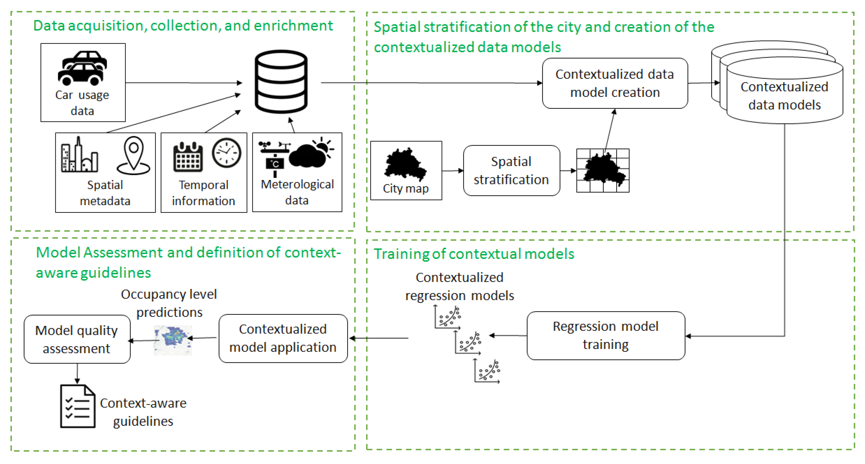
The presented methodology is depicted in Figure 1. It entails the following steps:

• Data acquisition, collection, and enrichment: the GPS positions of the cars of the FFCS system are acquired and stored at a given sampling rate. The acquired measurements are enriched with contextual descriptors including spatial and temporal information, meteorological conditions, and presence of Point of Interests.
• Spatial stratification of the city and creation of the contextualized data models: The urban area is spatially stratified into a grid of disjoint cells and each cell is characterized by the series of occupancy levels. Sampled data are clustered into groups according to the underlying context of generation in order to separately analyze FFCS usage data acquired in different scenarios.
• Training of contextual models: Prediction models are trained on each contextual data set separately for each area. Models include both Machine Learning-based algorithms and baseline methods. ML-based strategies consider multivariate data describing (i) a static neighborhood of the target cell including spatially close cells, (ii) a dynamic neighborhood including cells whose correlation with the target one based on trips is higher than expected, or (iii) exclusively the target area (i.e., cell-specific data model). Baselines assume stationary occupancy levels trends, predicting the last or the average occupancy levels over a bounded time window.
• Model assessment and definition of context-aware guidelines: The effectiveness of the models in predicting the occupancy levels in the near future is assessed on a test sample. According to the outcomes achieved in different contexts, a set of shared guidelines could be provided to the system managers.

3.1. Data Acquisition, Collection, and Enrichment

Free Floating Car Sharing (FFCS) Services track car movements across urban environments. To study car availability within restricted city areas, we acquire, store, and analyze FFCS usage data. More specifically, we first collect data about car bookings, which include rentals and parkings. Then, since the main purpose of the present study is to study short-term car availability within restricted urban areas, hereafter we will focus the analysis on the number of parked cars while neglecting data about actual rentals.

Let B be the set of bookings. A booking $b\in B$ is characterized by the car plate (which is the car identifier $id\left(b\right)$), origin/destination positions ($o\left(b\right)$ and $d\left(b\right)$), starting/ending time stamps ($t_s\left(b\right)$ and $t_e\left(b\right)$), its time duration ($t_d\left(b\right)=t_e\left(b\right)-t_s\left(b\right)$), its haversine distance [28] ($h_d\left(b\right)=haversine(o\left(b\right),d\left(b\right))$), and by the fuel consumption ($c\left(b\right)$).

Similar to the data model previously proposed in [21], a booking $b\in B$ is classified as a rental if the corresponding measurements clearly indicate that the car has moved across the city. To discover rentals, the following empirical conditions are verified: (i) the travelled distance is significant, i.e., 100 m $<h_d\left(b\right)<40$ km, (ii) the booking time duration is acceptable (2 min $<t_d\left(b\right)<2$ h), and (iii) the fuel consumption associated with the booking is above zero ($c\left(b\right)\ge 0$). We employ this filter to consider only one way trips within the operative area, discarding (i) bookings where the car did not move from the cell as the user cancel the reservation before using the car, (ii) maintenance operations that cause long lasting trips in which we cannot track the car location, and (iii) refueling carried out by the operator.

Starting from the rental dataset, we compute parking dataset to know the cars availability in the city in any given moment. Starting from the rental dataset, we compute its complementary information i.e., the parking event. Having two consecutive bookings b and $b+1$ for the same car, we check if the destination position $d\left(b\right)$ is the same as the origin position $o(b+1)$, if so we record the parking event p. We enforce this check since through the previous filter we discard some bookings and since we may have some missing data due to a data acquisition failure. Each parking $p\in P[P\subset B]$ is characterized by the car identifier ($ID\left(p\right)$), the location ($o\left(p\right)$), and by the starting/ending times ($t_s\left(p\right)$ and $t_e\left(p\right)$).

3.2. Spatial Stratification of the City Map

Spatial stratification of urban areas consists of dividing the space into areas to study the spatial heterogeneity of an observed phenomenon, i.e., understanding the extent to which the observations of the considered phenomenon are unevenly distributed across the areas [29,30]. Examples of previous applications of the aforesaid approach are given in [31,32,33,34].

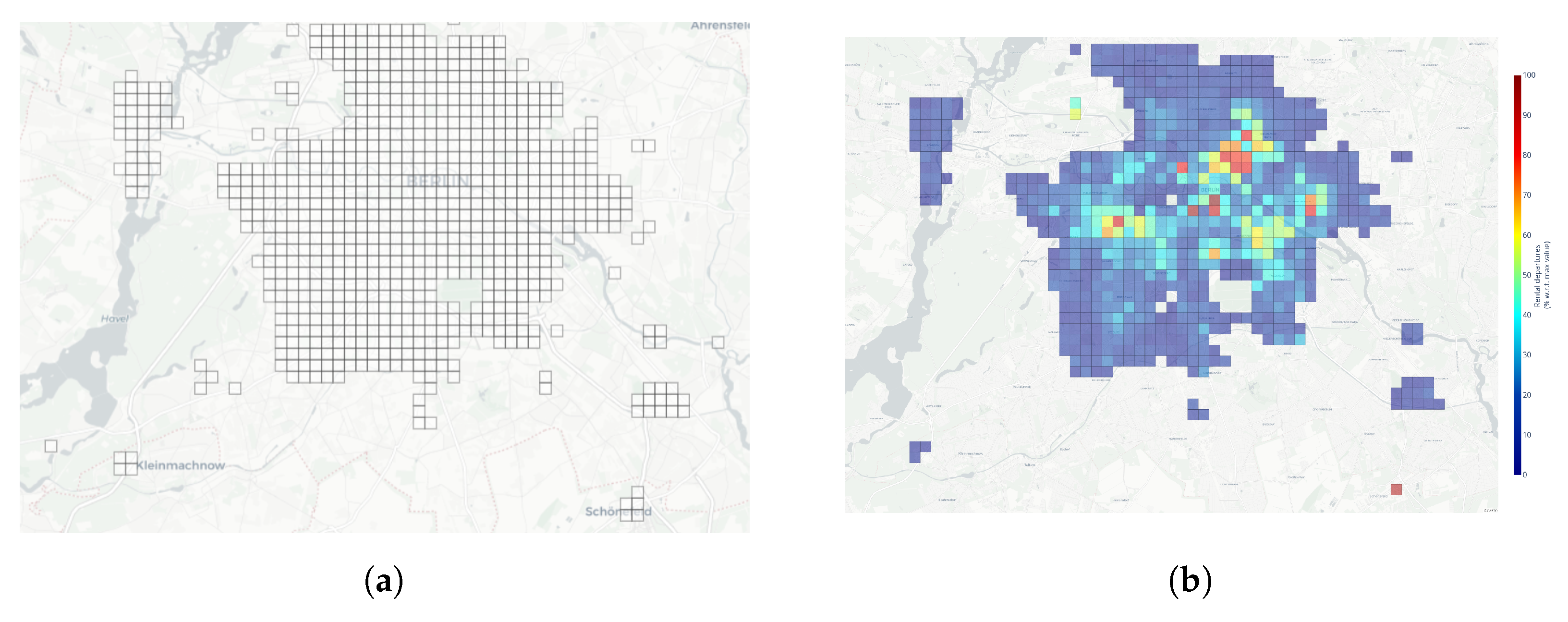
Our goal is to study the FFCS car movements across the urban environment. Since users are mainly interested in checking car availability within a restricted area, we use a grid to partition the city map into a set of disjoint squared cells of size 500 m × 500 m. The use of spatial stratification is established for coping with spatial data. Assuming that the user is already in the cell, with the adopted cell size, any car within the cell is at walking distance. Grid cells are mapped to parking data according to the GPS coordinates.

Let G be the $n\times m$ grid and let $C_{11},\dots ,C_{nm}$ be the identifiers of the corresponding grid cells. Without loss of generality, hereafter we will consider the grid cells as representative urban areas. However, the presented methodology can be trivially extended to arbitrary topologies.

Hereafter, we will consider Berlin as representative city because its FFCS service has the largest fleet in Europe. Figure 2a shows the grid defined on top of the city map of Berlin, while, in Figure 2b, the grid is overlapped by a colored heatmap showing the distribution of the rental departures in the operative city area. The values in the heatmap are normalized with respect to the maximum observed value, i.e., the zone having the highest number of rental departures. Interestingly, the heatmap highlights many highly popular cells, where it is very likely to have temporary car unavailability. The most popular cells are located within a relatively large perimeter, indicating that they are very attractive for users. The cell with the highest number of rentals includes the international airport, which is the source and destination of a significant number of car travels.

3.3. Data Enrichment with Contextual Information

Citizen demand of innovative services in Smart City environments is known to be related to their spatio-temporal context of use [35]. To enrich the data model with contextual information for each cell, we also consider the following external metadata $\mathcal{M}$:

• Temporal metadata (${\mathcal{M}}_{time}$): calendar data descriptors extracted from starting and ending times, i.e., date, weekday (Mon–Sun), hour of the day (0–24), 3-h daily time slot (e.g., from 6:00 a.m. to 9:00 a.m.), weekday, holiday/working day.
• Weather metadata (${\mathcal{M}}_{wea}$): meteorological data associated with the cell at the starting/ending times, i.e., temperature, humidity, wind speed,
• Spatial metadata (${\mathcal{M}}_{space}$): descriptors of the cell location in the city map (e.g., city center, suburbs, external hub), and
• Functional metadata (${\mathcal{M}}_{funct}$): descriptors of the main activities carried out in the cell based, for instance, on the presence of Points of Interests (e.g., restaurants, subway, and railway stations, airports) within the cell.

Each cell can be characterized in relation to the aforesaid metadata facets, which jointly contribute to characterize incoming and outgoing car travels for the target cell. More specifically, (i) the temporal context indicates when the prediction is performed, such as in a weekday or during the weekend. It is relevant to capture multi-resolution temporal trends in the analyzed data. (ii) The weather context denotes the meteorological conditions observed during the car travels. The idea behind is that the weather conditions in the urban area may affect the user habits thus influencing car rentals (e.g., users tend to use more the car when it rains). (iii) The spatial context describes where the cell is located, since neighbor cells can impact on arrival and departures from the target cell. (iv) The functional context describes what is the main activity carried out in the cell. For example, business and residential are examples of functional metadata values, which can be further specialized as workplaces and living houses, respectively. As previously discussed in [36,37], the POIs available in the cell are particularly suitable for describing car rentals within a cell.

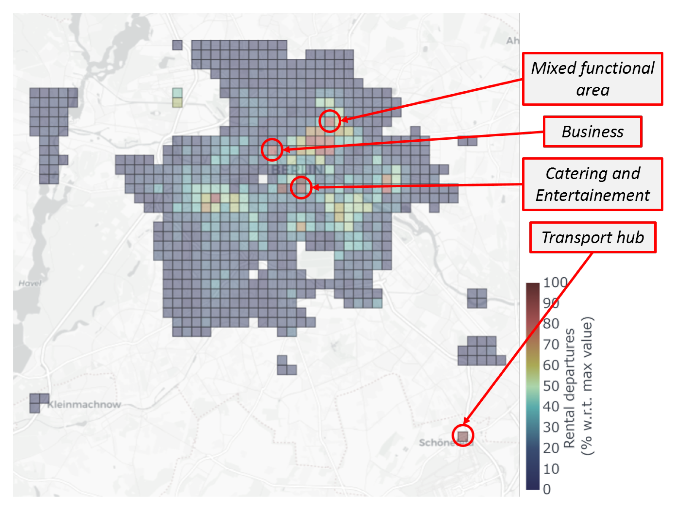
Below, we will report some examples of functional metadata descriptors as well as a selection of representative cells in Berlin annotated with them. The selected cells are highlighted in the heatmap shown in Figure 3.

• business (e.g., cells 25–30): workplace mainly occupied by headquarters of companies. The example use case for this category is a cell in Berlin including the headquarters of a company offering services such as real estate consultancy and insurance and a train station.
• catering and entertainment (e.g., cells 26–28): this area is characterized by a high density of services such as restaurants, pubs and hotels.
• mixed functional area (e.g, cells 31–33): this area characterized by many bar-restaurants, shops, and offices.
• transport hub (e.g., cells 0–45): this area is mainly devoted to a transport hub (e.g, airport).

3.4. Formalization of the Prediction Contexts

Since our goal is to predict the number of parked cars available at a certain time point within a specific cell, we first need to define the context in which the prediction will be performed. Then, we will build the data model tailored to the target cell and context, which will be used for prediction purposes.

Let T be the time period used to learn past trends in FFCS usage data and let $t_1$, …, $t_k$ be a sequence of k consecutive sampling points of time in T. For the sake of simplicity, $t_k$ is assumed to be the current sampling time, while $t_1$, …, $t_{k-1}$ are past time points in T. We will denote as occ($C_{ij}$,$t_s$) [$1\le i\le n$, $1\le j\le m$, $1\le s\le k$] the occupancy level of cell $C_{ij}$ acquired at time $t_s$. The prediction task entails forecasting the occupancy levels of the cell in the near future. We will denote as prediction time $t_p$ [$t_p>t_k$] the point of time for which the prediction is made. The gap between current and prediction time $\delta =|t_p-t_k|$ is usually denoted as prediction horizon.

The context of prediction for the target cell $C_{ij}$ is a combination of descriptor values from the metadata set $\mathcal{M}$ reported in Section 3.3. For example, a spatio-temporal context $\mathcal{C}$(${\mathcal{M}}_{time}$, ${\mathcal{M}}_{space}$) may combine temporal and spatial information. It may include FFCS usage data acquired from cells located in the city center during the weekend. The former context can be further specialized by considering only the cells including restaurants and cinemas $\mathcal{C}$(${\mathcal{M}}_{time}$, ${\mathcal{M}}_{space}$, ${\mathcal{M}}_{funct}$).

Defining the context of prediction is crucial for filtering out FFCS usage data that are not worth including in the data model. For example, the past car usage data acquired during the weekdays at lunchtime is probably not suitable for predicting the occupancy level of a cell at midnight during the weekend.

3.5. Context-Specific Data Model

The data model consists of the past occupancy levels of the target cell acquired in the reference time period T and stored into a unique repository. The underlying assumption is that past and current cell’s occupancy levels are likely to be correlated with the future ones, as car movements within the urban area are expected to show periodic trends.

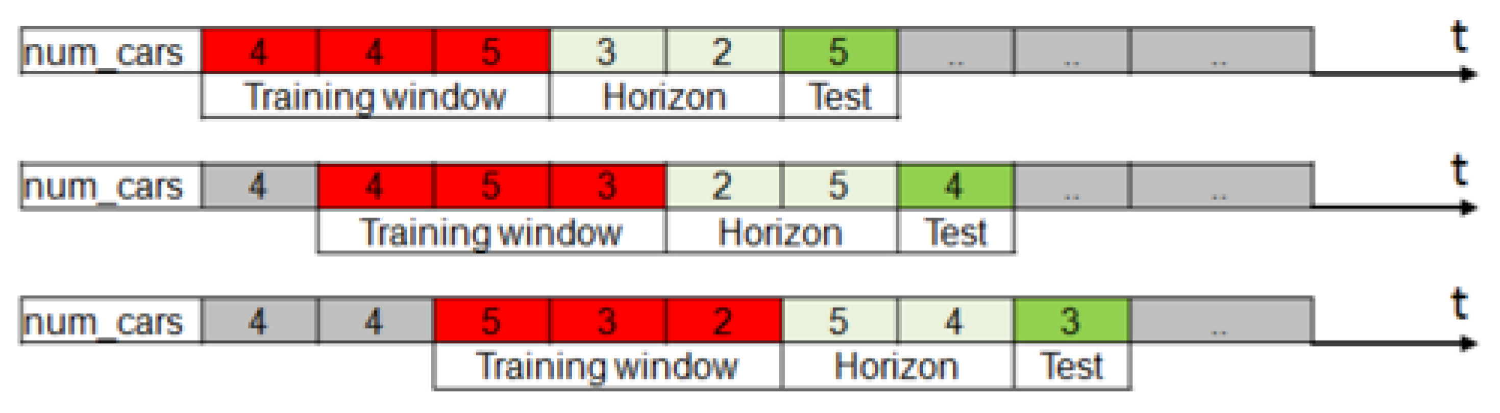
Since the occupancy levels of the same cell are likely to be correlated with each other, for each cell $C_{ij}$ and prediction time $t_p$, we consider the current and past values within a specified time window $TW$ (hereafter denoted as training window). The training window $TW$ slides over T in order to discover relevant correlations among temporarily close occupancy levels (see Figure 4). $TW$ consists of an ordered sequence of $T{W}_{size}$ points of time $t_k$, $t_{k-1}$, …, $t_{k-T{W}_{size}+1}$. For the sake of simplicity, hereafter we will assume a uniform sampling within $TW$, i.e., $\forall t_i,t_{i-1}\in TW$ the sampling interval $\Delta$ = $t_i-t_{i-1}$ is fixed.

For each prediction time $t_p$, we collect also the occupancy levels acquired from the neighbor area of the target cell within the training window. The number of cars parked in nearby cells could be a relevant predictor for the occupancy level of the target cell. The idea behind this is that significant variations of the past and current occupancy levels of nearby cells could influence, to some extent, the future occupancy level of the target cell. In fact, the presence of cars in the neighbor area may reveal the presence of potential car movements towards the target cell in the near future. We model the neighbor area of a target cell as two square frames surrounding the cell. Specifically, (i) a first nearest frame (of 4 km${}^2$) and (ii) a second surrounding frame (of 16 km${}^2$), respectively.

Each record in the training data set corresponds to a different sliding training window $TW$ in T enriched with the corresponding occupancy level at the prediction time (known for training data only). Specifically, the following values are stored: (i) The occupancy levels related to the training window occ($C_{ij}$,$t_s$) [$k\le s\le k-T{W}_{size}+1$]; (ii) The occupancy level at prediction time occ($C_{ij}$, $t_p$).

3.6. Training of Contextualized Models

On top of the context-specific data models, we explore the use of various predictors, based on Machine Learning and not. This section thoroughly describes the strategies used to forecast the future occupancy levels for each cell and context.

We split the prediction models into two main classes, namely the baseline methods, which do not rely on ML, and the regression methods, which include both univariate and multivariate ML-based models.

Baseline methods. We consider the following baseline strategies:

• Predict the last value: Assuming a stationary trend for the time series of occupancy levels, it predicts the most recent value.
• Predict moving average: It exploits the moving average with P periods to model the underlying series trend. It predicts the moving average of the latest P samples as future occupancy level.

Regression methods. Regression algorithms study the underlying relationships and the causal effects between a set of predictive features in the training data model and the target class, i.e., the future occupancy level of the cell [28]. The values of the target class are assumed to be known in the training data, on top of which a model is learnt.

When the regressor considers only the series of past and current occupancy levels of the target cell, the prediction model is denoted as univariate. Conversely, when the regressor considers additional predictive features beyond the target variable, the regression model is denoted as multivariate.

We explore the use of three different kinds of multivariate regression models:

• Cell-Specific (CS): the data model exclusively includes the information about the target cell, including contextual information (see Section 3.5).
• Cell-Specific enriched with static neighborhood (CS + S): the data model includes the information not only about the target cell but also about the cell neighborhood.
• Cell-Specific enriched with dynamic neighborhood (CS + D): the data model includes all the information about the target cell and a selection of cells with correlated occupancy levels.

The input variables considered in the regression models consist of the occupancy levels of the cells in the sliding training window, in compliance with the data model described in Section 3.5. Specifically, the training dataset for the CS model contains one attribute for each past and present occupancy level of the target cell within the training window. The CS + S and CS + D datasets are extended versions of the former CS dataset, where the attributes considered for the target cell are replicated for each neighbor cell under consideration.

Since the temporal (${\mathcal{M}}_{time}$) and weather (${\mathcal{M}}_{wea}$) metadata reported in Section 3.3 are also useful to predict the occupancy level of the target cell, the training dataset also contains one attribute for each temporal and weather metadata.

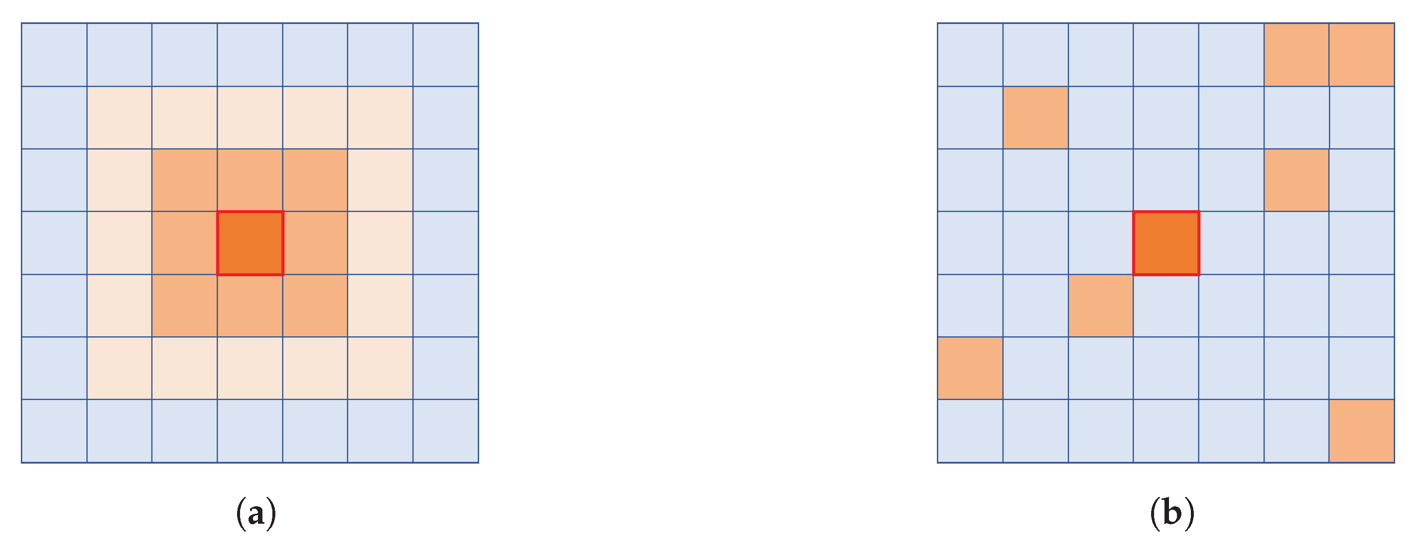
Figure 5a,b exemplify the procedures used to generate the neighborhood of a cell in the CS + S and CS + D strategies, respectively. The idea behind the model with static neighborhood is that, thanks to spatial proximity, nearby cells are likely to show correlated occupancy levels over time. Thus, they could be deemed as reliable predictors. Conversely, the model with dynamic neighborhood focuses the attention on a selection of cells, not necessarily located nearby, showing recurrent car movements towards or from the target cell.

In the CS + S strategy, we model the neighbor area of the target cell as two square frames surrounding the target cell itself (see Figure 5a). The static neighborhood is generated from the square frames described in Section 3.5. Specifically, it consists of a first nearest square frame including its neighbor cells (500 m from $c_i$) and a second square surrounding frame (1 km from $c_i$).

The dynamic neighborhood is selected based upon the rule-based strategy detailed in Section 3.7.

3.7. Identification of the Dynamic Neighborhood: An Association-Based Approach

We perform a preliminary correlation analysis between the occupancy levels of the neighbor cells and those of the target cell on training data (within the considered training window). The aim is to identify a subset of neighbor cells whose historical values are worth considering in the training phase of the multivariate regressors.

In principle, all the cells in the city map may retain a certain degree of correlation with the target cell because car movements from/to the target cell may be associated with arbitrary origins/destinations. However, incorporating the information about all the cells in the multivariate regression model would be counterproductive due to the well-known curse of dimensionality [38]. Hence, there is a need to identify a subset of most correlated cells in the neighborhood to include in the data model. This section presents the approach used to dynamically select the most correlated cells according to Cell-Specific enriched with dynamic neighborhood (CS + D) strategy.

The key idea is to explore the raw data about FFCS car trips in order to identify the cells producing a significant number of car movements, either towards or from the target cell. To tackle this issue, we apply association rule mining techniques [39] to discover and rank reliable associations among cell pairs. In our context, a trip is modeled as a pair of starting and ending cells. We collect all trip data associated with the same context into a separate dataset in order to discover context-specific correlations among cells. To our purposes, in the analyzed dataset, we disregard trip directions since both departure and arrivals to the target cell are worth considering to identify the neighbor cells of interest.

Association rules [39] represent recurrent co-occurrences between cells in the trip dataset. We apply the established Apriori association rule mining algorithm [40] to automatically extract all the associations $AR$: $C_{ij}\to C_{qz}$, where $C_{ij}$ and $C_{qz}$ is an arbitrary cell pair.

Association rule mining is typically driven by mining support and confidence thresholds [39]. The support index indicates the observed frequency of occurrence of the cell pair in the trip dataset. It is commonly used to discard low-quality patterns because they represent infrequent cell combinations. The confidence index of rule $C_{ij}\to C_{qz}$ is the conditional probability of occurrence of cell $C_{qz}$ in the trip dataset given the occurrence of cell $C_{ij}$. It indicates the strength of the association. However, to avoid discriminating between cell origin and destination, we decide to use a variant of the confidence index, called lift [28], which indicates the pairwise correlation between the cells. Its mathematical expression follows:

$$Lift(C_{ij}\to C_{qz})=\frac{conf(C_{ij}\to C_{qz})}{sup\left(C_{qz}\right)}$$

(1)

where $conf(C_{ij}\to C_{qz})$ is the rule confidence, whereas $sup\left(C_{qz}\right)$ is the observed frequency of occurrence of cell $C_{qz}$ in the trip dataset.

Lift values fall in the range (0, $+\infty$). A lift value greater than one indicates a positive correlation between the considered cells, whereas a value less than one corresponds to a negative correlation.

To identify the cells that are most correlated with the target one, we first mine the association rules including the target cell $C_{ij}$ (e.g., $C_{ij}\to C_{qz}$ or $C_{qz}\to C_{ij}$) and satisfying a minimum support threshold equal to 1%, a minimum confidence threshold equal to 50%, and a lift value greater than 1. Then, we rank rules by decreasing lift value, select the top ranked one, and identify the subset of most correlated cells accordingly. The number of selected cells can be specified by the analysts. In our experiments, we used 10 as a reference value, which is comparable to the number of cells included in the static frame. Notice that, since the extracted rules change from one context to another, the subset of selected cells could change as well.

3.8. Model Assessment and Definition of Context-Aware Guidelines

The presented framework enables the exploration of a variety of solutions to predict short-term cell occupancy levels. The solutions range from simple baseline methods (e.g., predict the last value, predict the moving average) to more advanced ML-based solutions, i.e., multivariate regression models.

A practical use case for the proposed system is the data-driven exploration and comparison of different solutions tailored to each cell and context. More specifically, system managers could identify the most appealing scenarios of usage for the prediction models in terms of monitored areas and spatio-temporal contexts. The effectiveness of the proposed strategies can be assessed on a separate test set, i.e., a portion of parking data exclusively devoted to performance evaluation.

Based on the achieved results, system managers could derive context-aware guidelines useful for tailoring the setup and usage of the intelligent system to the actual context. For each urban area and context, guidelines may indicate

• the type of prediction model (ML vs. baseline) that is most likely to be effective in predicting short-terms car occupancy levels.
• the recommended prediction horizon.
• the specific ML model sub-type (e.g., cell-specific, static neighborhood, dynamic neighborhood) or, alternatively, the most promising baseline method.
• in case ML-based approaches outperform baseline methods:

  –

  the recommended ML algorithm

  –

  the best algorithm configuration identified by grid search on historical FFCS usage data.

4. Experimental Results

This section summarizes the main empirical outcomes of the present study. It covers the following aspects:

• Experimental design: Description of data sources, algorithm configuration setting, and evaluation strategies. The goal is to clarify the evaluation procedures and make the set of ML pipeline repeatable as much as possible (see Section 4.1).
• Comparison between ML and baseline methods: Evaluation of the performance of the proposed prediction models in various spatio-temporal contexts. The goal is to identify the contexts in which ML-based approaches are worthy of consideration in place of simple baseline methods (see Section 4.2).
• Comparison between different ML-based approaches and regression algorithms: Comparison between the presented ML approaches in terms of both adopted strategy (cell-specific, static neighborhood, dynamic neighborhood) and regression algorithm. The idea is to gain insights into the configuration of the ML process (whenever necessary) and to figure out the corresponding guidelines in light of the achieved results (see Section 4.3).
• Comparison among data models: Evaluation of the impact of the functional contexts of cells and the prediction horizon on the average prediction error (MAE) achieved when using the three proposed data models (i.e., CS, CS + S, and CS + D) (see Section 4.4).
• Qualitative analysis of the extracted cell associations: Exploration of the extracted association rules in the contexts where ML-based approaches with dynamic neighborhood turned out to be more effective than the other approaches (see Section 4.5).
• Complexity analysis: Empirical evaluation of the complexity of the entire FFCS usage data analytics pipeline (see Section 4.6).
• Evaluation of time series stationarity: Analysis of the input data to investigate the non-stationarity of the time series. The goal is to corroborate the needs of ML-based regressions models rather than simpler autoregressive models (see Section 4.7).

4.1. Experimental Design

Data. We analyzed a one-year-long parking dataset collected using the UMAP tool [41]. The dataset reports all the bookings in all the cities where Car2Go provides its service. Notice that the use of the Car2go API to acquire these data (https://www.car2go.com/api/tou.htm) is subject to approval by Car2go. We got the approval from September 2016 until end of January 2018. Among the different cities available in the dataset, Berlin has been considered as a reference use case for the present study because it includes cells with rather variable trends, ranging from stationary series to highly non-stationary occupancy level variations. Hence, it was deemed as an interesting case study to assess the capability of the system to support the generation of context-aware guidelines.

The service provider has exposed ad hoc APIs through which the GPS positions of the 1k vehicles for rent can be crawled every minute. For the sake of simplicity, hereafter we will focus our exploration on the historical data acquired in year 2017. In this study, we report the results obtained considering a representative time period (i.e., September and October). In this period, we record 626k bookings, resulting in 390k rentals after discarding cancellations and long lasting trips, and 380k after removing refueling operations. These rentals allow us to correctly track 372k parking events describing the car location while parked and available for the customers.

To crawl weather data we exploited the Application Programming Interfaces exposed by [42]. To identify the POIs located in the urban area, we exploited the OpenStreetMap service [43].

Based on the collected data, we built the training dataset that we exploit to train the regression algorithms. The variables used to train the regression models are those reported in Section 3.6.

Algorithms. We integrated the following regression algorithms: (i) Lasso, (ii) Linear Regression (LR), (iii) Random Forest (RF), and (iv) Gradient Boosting Tree (GBT). More details on the prediction algorithms are given in [38].

To fit the models to the analyzed data, we performed a grid search. The selected configuration settings are given below. More details on the regression functions can be found in [44]:

• Random Forest (RF): n_estimators = 50, max_features = sqrt, min_samples_split = 5, min_samples_leaf = 5, max_depth = 10
• Gradient Boosting Tree (GBT): learning rate = 0.1, n_estimators = 100, max_depth = 1, loss = lad
• Lasso: alpha = 1
• Linear regression (LR): fit_intercept = true, normalize = true

To run the experiments, the prediction horizon has been set to 3 h and the size of the training window to 21 days. The impact of the two parameters has been analyzed in Section 4.2.3.

Validation. To validate the performance of each regression algorithm, we apply a train-test procedure by sliding the training window and the test over the whole period to perform day-by-day predictions. The prediction errors achieved over the entire period are averaged to summarize the algorithm performance based on the standard Mean Absolute Error (MAE) measure [38]. The MAE measures the difference between the number of cars estimated by the regression algorithm at prediction time $t_p$ for the target cell and the actual number of cars available in the cell at $t_p$. Analogously, the MAE value is used to evaluate the prediction accuracy when using the baseline solution.

The experiments were run on a quad-core 3.30 GHz Intel®Xeon workstation (Manufacturer location: Santa Clara, CA, USA) with 16 GB of RAM with Ubuntu Linux 13.10 LTS.

4.2. Machine Learning vs. Baseline Approaches: A Statistical Comparison

We performed an empirical comparison between ML-based and baseline methods in different contexts. Hereafter, we will report the outcomes of two representative temporal contexts, i.e., weekdays (from Monday to Friday) and weekend days (Saturday and Sunday). The aforesaid contexts are deemed as suitable for exploring scenarios with a high variance in the cell occupancy levels.

4.2.1. Comparison in Different Temporal Contexts

Table 1. Comparison between ML-based and baseline solutions in terms of MAE (avg ± std).

	Temporal Context
	Weekday				Weekend Day
	Baseline		ML		Baseline		ML
Functional Context	Last Value	Moving Average	RF	Data Model	Last Value	Moving Average	RF	Data Model
Business	2.11 ± 0.86	2.39 ± 1.06	1.51 ± 0.49	CS + D	1.11 ± 0.42	1.10 ± 0.54	2.68 ± 0.87	CS + D
Catering and Entertainment	3.45 ± 1.35	4.34 ± 1.84	2.43 ± 0.99	CS + D	2.60 ± 1.50	3.16 ± 2.14	1.40 ± 0.30	CS + D
Mixed functional area	1.71 ± 0.53	1.81 ± 0.65	1.49 ± 0.36	CS + S	1.18 ± 0.13	1.11 ± 0.12	1.20 ± 0.37	CS + S
Transport hub	6.47 ± 2.26	8.38 ± 2.93	4.10 ± 1.67	CS	6.38 ± 2.37	8.59 ± 3.22	5.25 ± 3.13	CS

shows the MAE achieved by the best performing ML-based approach (i.e., Random Forest regressor, (RF)) and the two baseline strategies (predicting the last value or the moving average, respectively) in the temporal contexts weekday and weekend. For the sake of brevity, we reported the results achieved on the four cells chosen as representative of different functional contexts (see Section 3.3). For each cell, Table 1 also indicates the most effective data model (i.e., CS, CS + S, or CS + D).

From the comparison between the two baseline strategies, selecting the Last value approach has shown to be the most accurate one because it performed best for three cells out of four (i.e., except for cell business) in temporal contexts weekday and in for two cells out of four in the temporal context weekend day (i.e., except for cells business and transport hub).

The ML-based approach has shown to be significantly more accurate than the baseline in most case for the temporal context weekday. Conversely, over the weekend baseline predictors achieved better performance than ML, except for in the transport hub where the ML-based approach gave the best results. The performance improvements were evident in all considered functional contexts except for category mixed functional area, where the MAE gaps were rather limited. Weekdays are temporal contexts where cells are usually characterized by a significant variance in the occupancy level. The prediction task being more challenging, ML-based models seem to the most appropriate solution. Conversely, when the variance in the occupancy levels gets lower, as in weekend days, baseline methods achieve comparable or even better performance even if they rely on much simpler models. The occupancy levels of cell transport hub are quite variable in both temporal contexts, mainly due to presence of the Berlin international airport. This could explain the significantly better performance achieved by ML-based approaches compared to baselines.

To validate the statistical significance of the MAE improvement achieved by the ML-based approach, we applied the paired t-test [45]. The test was applied at significance level p = 0.05 on all the evaluated datasets. When comparing ML-based with baseline approach, the paired t-test confirms the statistical significance of all the MAE improvements. The outcomes of the statistical validation confirm that the performance of ML-based approaches are superior to those of baseline methods in the most challenging functional and temporal contexts (i.e., when the variance of the occupancy levels is fairly high). For the weekend days, the paired t-test indicates that the (limited) performance gap is statistically significant for cell business but not for cells catering and entertainment and mixed functional area.

To broaden the scope of the empirical validation phase, we also reported in

Table 2. Comparison between ML-based and baseline solutions on a larger cell selection for each functional context, in terms of MAE (avg ± std).

	Temporal Context
	Weekday				Weekend Day
	Baseline		ML		Baseline		ML
Functional Context	Last Value	Moving Average	RF	Data Model	Last Value	Moving Average	RF	Data Model
Business	2.61 ± 0.95	2.52 ± 1.00	1.96 ± 0.67	CS + D	1.36 ± 0.44	2.04 ± 1.06	1.37 ± 1.78	CS + D
Catering and Entertainment	1.54 ± 0.59	2.35 ± 0.94	1.34 ± 0.43	CS + D	1.82 ± 0.83	1.36 ± 0.53	1.78 ± 0.53	CS + D
Mixed functional area	1.30 ± 0.40	1.31 ± 0.46	1.22 ± 0.31	CS + S	1.26 ± 0.33	1.26 ± 0.34	1.21 ± 0.37	CS + S
Transport hub	3.82 ± 2.43	4.88 ± 3.04	2.58 ± 1.81	CS	3.58 ± 2.13	4.76 ± 2.78	3.01 ± 2.32	CS

the average MAE achieved on a larger cell selection, i.e., the top-3 cells in terms of variance separately for each functional context. The results are in line with those achieved on the reference cells.

4.2.2. Comparison on Fine-Grained Temporal Contexts

Considering fine-grained time granularity allows us to deepen the performance comparison between ML-based and baseline solutions. Of course, a drill down to fine-grained data increases the variance in the cell occupancy levels because the data model becomes more sensitive to small fluctuations occurred along the day. Hence, ML-based approach are supposed to be the most promising solutions since they are able to capture non-stationary and complex trends.

Taken as a whole, the experimental results confirm the expectations. Specifically, the results achieved on a representative subset of cells and reference time slots are summarized in

Table 3. Comparison between ML-based and baseline solutions in terms of MAE (avg ± std) for different time slots on weekdays.

	Weekday-Time Slot
	Morning		Afternoon		Evening		Night
Functional Context	Baseline	ML	Baseline	ML	Baseline	ML	Baseline	ML
Business	Last Value	RF (CS + D)	Last Value	RF (CS + D)	Last Value	RF (CS)	Last Value	RF (CS)
	3.77 ± 2.17	2.71 ± 1.33	1.75 ± 1.72	1.72 ± 2.16	0.67 ± 0.62	0.43 ± 0.33	0.39 ± 0.41	0.50 ± 0.43
Transport hub	Last Value	RF (CS)	Last Value	RF (CS + D)	Last Value	RF (CS)	Last Value	RF (CS)
	5.91 ± 2.83	5.80 ± 3.23	4.18 ± 3.36	5.37 ± 3.34	7.55 ± 7.01	2.87 ± 3.32	5.20 ± 7.29	1.14 ± 1.64

and

Table 4. Comparison between ML-based and baseline solutions in terms of MAE (avg ± std) for different time slots on weekend days.

	Weekday-Time Slot
	Morning		Afternoon		Evening		Night
Functional Context	Baseline	ML	Baseline	ML	Baseline	ML	Baseline	ML
Business	Last Value	RF (CS)	Last Value	RF (CS + S)	Last Value	RF (CS + D)	Last Value	RF (CS)
	3.85 ± 2.36	6.39 ± 2.41	4.45 ± 3.25	2.90 ± 3.00	0.86 ± 0.44	0.47 ± 0.09	0.26 ± 0.20	0.40 ± 0.30

, respectively. We considered the following 3-h daily time slots: morning (6–9), afternoon (12–15), evening (18–21), and night time (21–24). For cells business and transport hub, the ML-based solution performed better than baseline while averaging the prediction outcomes at the daily frequency (see Table 1). However, the baseline solution (slightly) improves ML on specific daily time slots (i.e., evening for business and morning for transport hub). Analogously, for cell business, the baseline solution is more accurate than ML-based approach during weekend days, whereas ML performed best on time slots afternoon and evening.

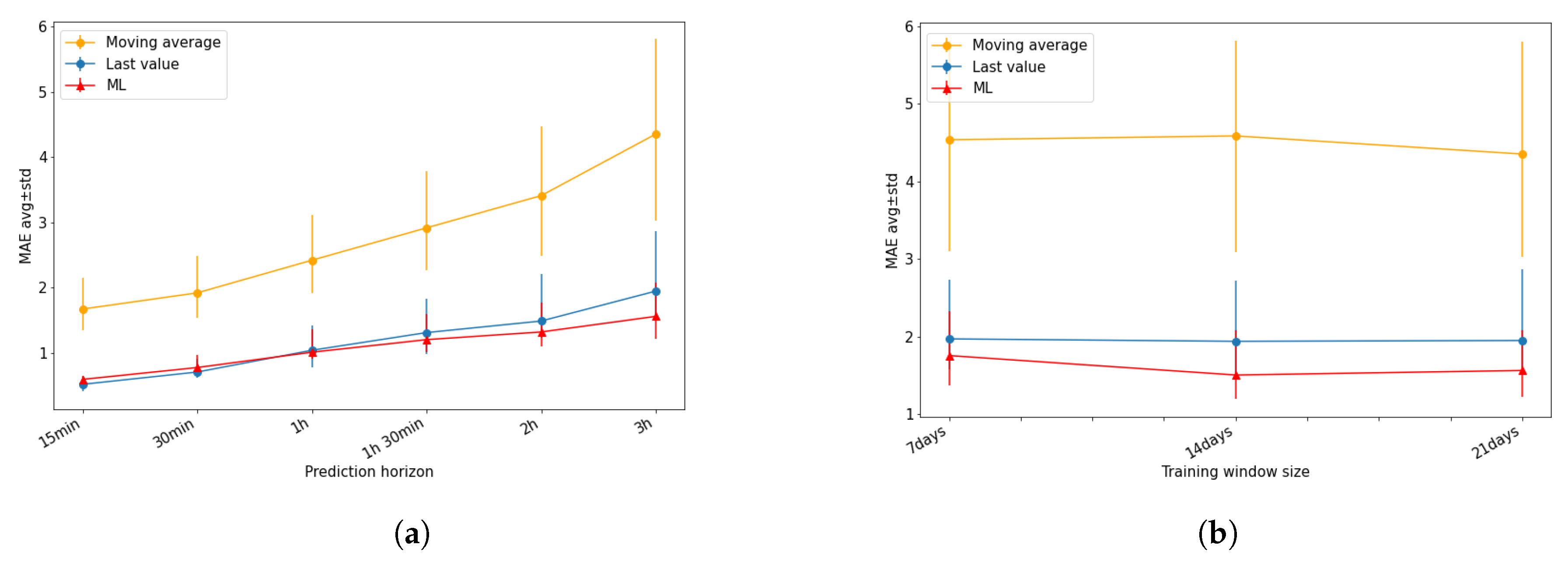
4.2.3. Comparison for Different Prediction Horizons and Training Window Sizes

Figure 6a summarizes the results of the comparison betwewen ML-based (i.e., Random Forest regression (RF)) and baseline solutions performed by varying the value of the prediction horizon. The strategy named Predict the last value performs (slightly) better than the ML-based solutions by setting small horizon values (e.g., 1 h), where the latter ones performed best (in terms of mean MAE value and standard deviation) while increasing the prediction horizon. Conversely, the baseline strategy relying on moving average achieved the worst results.

The impact of training window size in comparing baseline and ML-based solutions (i.e., Random Forest regression) is shown in Figure 6b. The baseline strategy (Last value) and ML-based solution have comparable performance for a short training window, but ML-based solutions performs better (in terms of both mean and standard deviation values MAE) when increasing the training window size.

4.3. Comparison between Different ML-Based Approaches and Regression Algorithms

Table 5. Comparison between ML-based algorithms in terms of MAE (avg ± std).

	Temporal Context
	Weekday				Weekend Day
Functional Context	RF	GBT	LR	Lasso	RF	GBT	LR	Lasso
Business	1.51 ± 0.49	1.54 ± 0.55	1.91 ± 0.65	1.72 ± 0.58	2.68 ± 0.87	2.54 ± 1.07	3.09 ± 0.66	2.89 ± 0.87
	CS + D	CS + D	CS + D	CS + D	CS + D	CS + S	CS	CS + S
Catering and Entertainment	2.43 ± 0.99	2.66 ± 1.00	3.04 ± 0.95	2.99 ± 0.92	1.40 ± 0.30	1.61 ± 0.34	1.45 ± 0.33	1.51 ± 0.26
	CS + D	CS + D	CD + D	CS + D	CS + D	CS + S	CS	CS + S
Mixed functional area	1.49 ± 0.36	1.51 ± 0.33	1.53 ± 0.37	1.65 ± 0.39	1.20 ± 0.37	1.14 ± 0.25	1.29 ± 0.37	1.65 ± 0.39
	CS + S	CS + S	CS	CS + S	CS + S	CS + D	CS	CS + S
Transport hub	4.10 ± 1.67	4.66 ± 1.70	5.32 ± 1.51	5.29 ± 1.58	5.25 ± 3.13	6.04 ± 2.75	6.97 ± 1.82	6.55 ± 2.20
	CS	CS + D	CS + D	CS + D	CS + S	CS + S	CS + D	CS + D

reports the results of the comparison between different regression algorithms. The experimental results show that Random Forest regressor (RF) performed significantly better than Lasso and LR algorithms. The performance improvements were more significant in cells catering and entertainment and transport hub, in particular when considering weekday, and in cells business and transport hub for weekend days.

RF and GBRT algorithms achieved comparable performance, but RF always overperformed GBRT except for two cases (i.e., cells business and mixed functional area for weekend day).

4.4. Comparison among Data Models

This section analyzes the impact of the functional contexts of cells and the prediction horizon on the average prediction error (MAE) achieved when using the three proposed data models (CS, CS + S, or CS + D) to train the best performing ML-based solution (i.e., Random Forest regression (RF)).

4.4.1. Impact of the Functional Context on the Data Models

Table 6. Comparison of the data models for different functional contexts, in terms of MAE (avg ± std).

	Temporal Context
	Weekday			Weekend Day
Functional Context	CS	CS + S	CS + D	CS	CS + S	CS + D
Business	1.63 ± 0.55	1.67 ± 0.74	1.51 ± 0.49	2.73 ± 0.91	2.71 ± 0.94	2.68 ± 0.87
Catering and Entertainment	2.47 ± 0.97	2.57 ± 1.17	2.43 ± 0.99	1.44 ± 0.35	1.53 ± 0.38	1.40 ± 0.30
Mixed functional area	1.51 ± 0.28	1.49 ± 0.36	1.50 ± 0.42	1.44 ± 0.60	1.20 ± 0.37	1.22 ± 0.37
Transport hub	4.10 ± 1.67	-	4.14 ± 1.71	5.25 ± 3.13	-	5.37 ± 3.06

compares the MAE value for the three proposed data models when applied for each functional context, in the temporal contexts of weekday and weekend.

For business and catering and entertainment cells, the ML-based solution provides better performance when trained using the Cell-Specific enriched with the dynamic neighborhood data model. Instead, for the mixed functional area cells, the most accurate solution is given by the Cell-Specific enriched with static neighborhood data model. Thus, the occupancy levels of cells are, on average, fairly correlated with faraway cells in the former case, while with nearby cells in the latter case. For isolated cells (transport hub cells), the ML-based solution achieved best performance when trained by considering only the occupancy levels of the target cell (Cell-Specific data model).

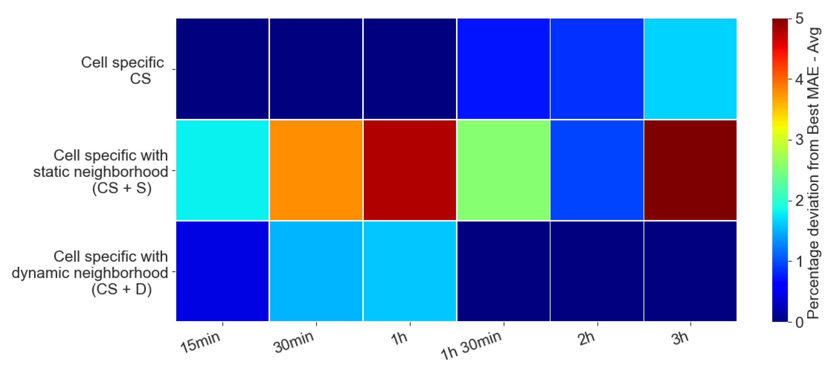
4.4.2. Impact of the Prediction Horizon on the Data Models

The heatmap in Figure 7 shows the combined effect of data models and prediction horizon $\delta$ on the average prediction error (MAE). As a representative example, we considered cell business and Random Forest as regression algorithms.

Each heatmap cell corresponds to a different combination of prediction horizon value (x-axis) and data model (y-axis). Increasing values of prediction horizon are reported on the x-axis. Consider a horizon of prediction $\delta$ and the associated column in the heatmap. Cell color indicates the average MAE value normalized by the value of the best performing data model for that horizon. The color of the heatmap cell ranges from dark red to dark blue depending on whether the MAE value for the data model in the cell is closer (darker blue) or more distant (darker red) from the best performing solution for the same horizon.

When the prediction horizon value is short (up to 1 h), the best data model relies only on the information about the target cell. Thus, the occupancy levels of the target cell provide sufficient information for making prediction. When the prediction horizon increases, the most accurate data model includes the dynamic neighbor. Hence, in the latter and more challenging scenario, the occupancy levels of neighbor cells matter. The data model with static neighbor performed worse than the dynamic neighbor model. Since surrounding cells are all in the headquarter of big company, the model was unable to capture significant trends in FFCS usage data.

4.5. Qualitative Analysis of the Extracted Cell Associations

Table 7. Examples of associations used to build the dynamic neighborhoods for cell catering and entertainment on Monday morning and on Monday afternoon.

Monday Morning		Monday Afternoon
Cell	Lift	Cell	Lift
22–18	20.2	41–29	18.2
40–26	15.1	10–27	7.3
15–26	9.0	30–34	6.6
29–16	8.1	23–32	6.1
17–31	7.3	25–12	5.6
40–29	7.3	22–16	5.2
10–26	6.2	35–31	4.9
41–27	5.0	27–31	4.8
30–38	5.0	33–32	4.7
40–30	4.5	21–29	4.6

reports for a representative cell (catering and entertainment) the identifiers of the top-10 most correlated cells selected by the Cell-Specific enriched with dynamic neighborhood (CS + D) strategy in two different contexts, i.e., Monday morning and Monday afternoon. For each association, it also reports the corresponding lift value, which expresses the strength of the cell correlation.

The neighbor cells selected by means of the association rule mining approach are those occurring in the top ranked associations. Since the dynamic neighborhood is context-specific, different rules and cells have been identified in the two considered contexts (see, for instance, Column 1 and Column 3 of Table 7). Even if the target cell is the same, FFCS service usage patterns are rather different. The rule-based model allows the prediction model to take contextual diversity into account.

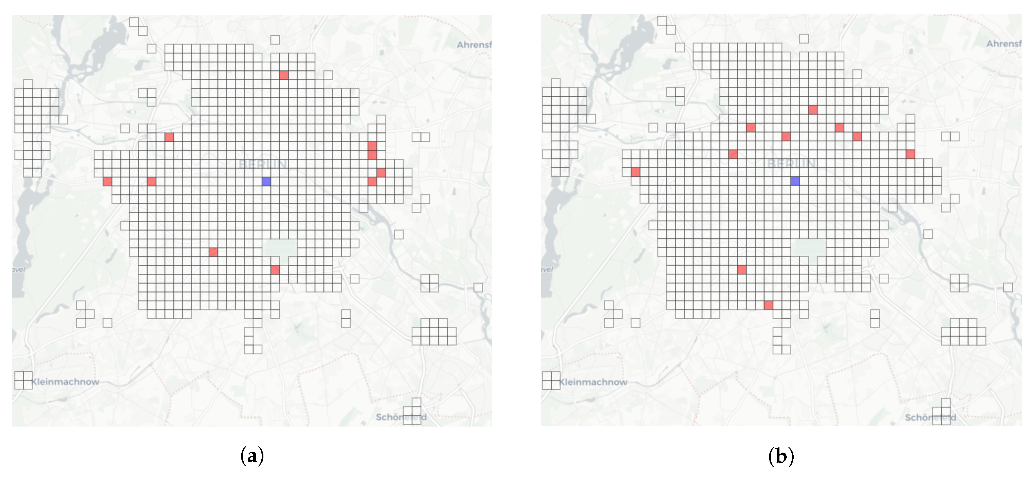
Figure 8a,b depict the dynamic neighborhoods generated by means of the association rules and the selected cells reported in Table 7. The blue cell is the target one while the red ones are the content of the dynamic neighborhood. We can notice that the dynamic neighborhoods are not influenced by the proximity of the selected cells with respect to the target one. This is reasonable because, in some contexts, the cars are used to move from relative faraway locations. For example, in the morning, many users rent a car to commute for work. Trip destinations are relatively faraway (see, for instance, the red cells in Figure 8a). Conversely, in the afternoon, many users rent a car from the city center to move towards catering and entertainment cells, which are relatively close to the trip departure (see Figure 8b).

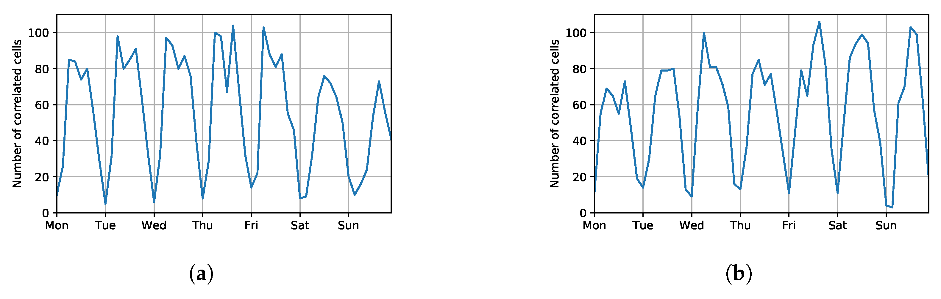
Finally, we analyzed the number of cells that are deemed as correlated with the target one in terms of car trips for various days of the week and time slots. They refer to the complete sets of correlated cells which have been identified before selecting the top-k ones in order to create the dynamic neighborhoods. Figure 9 summarizes the results achieved for the catering and entertainment and business cells. In both cases, the number of correlated cells decreases in periods of limited service usage (e.g., in the early morning). This is due to the fact that most of the cell combinations are deemed as not statistically relevant by the association rule mining algorithm.

4.6. Complexity Analysis

We analyzed the time complexity of the pipeline of FFCS usage data analytics described in Section 3.

The most time- and memory-consuming step in the designed pipeline is the training of contextualized models. When it relies on ML-based approaches, it entails training multiple regression models on historical data. In the experiments performed on Car2Go Berlin data, we have defined four different functional contexts (business, catering and entertainment, mixed functional area and transport hub), two temporal contexts, and three data models (cell specific, cell specific with static neighborhood and cell specific with dynamic neighborhood). When baseline methods perform best, training time is negligible. Conversely, training ML models took between 5 s (for Lasso model) to 60 s (for Random Forest model). The time and memory cost to apply the ML-based models to test data are at least one order of magnitude lower than the training phase (5 s in the worst case).

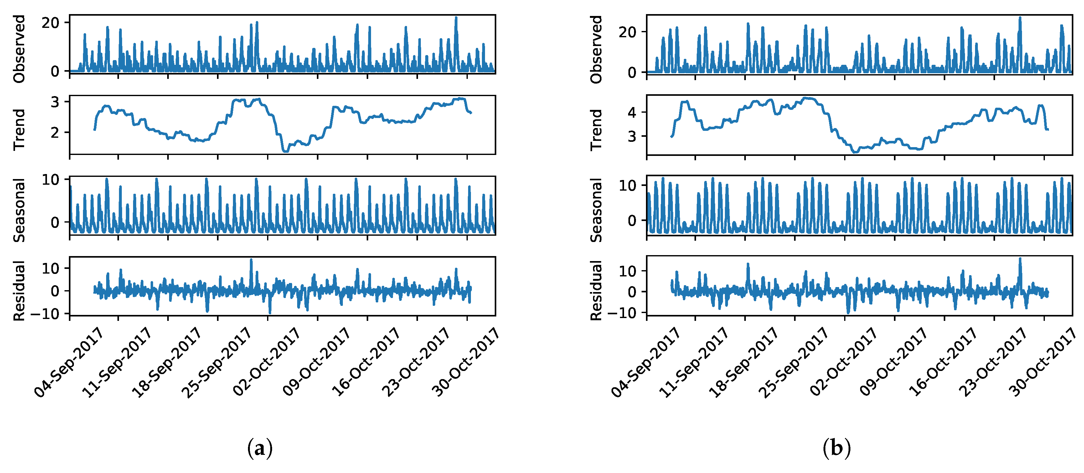
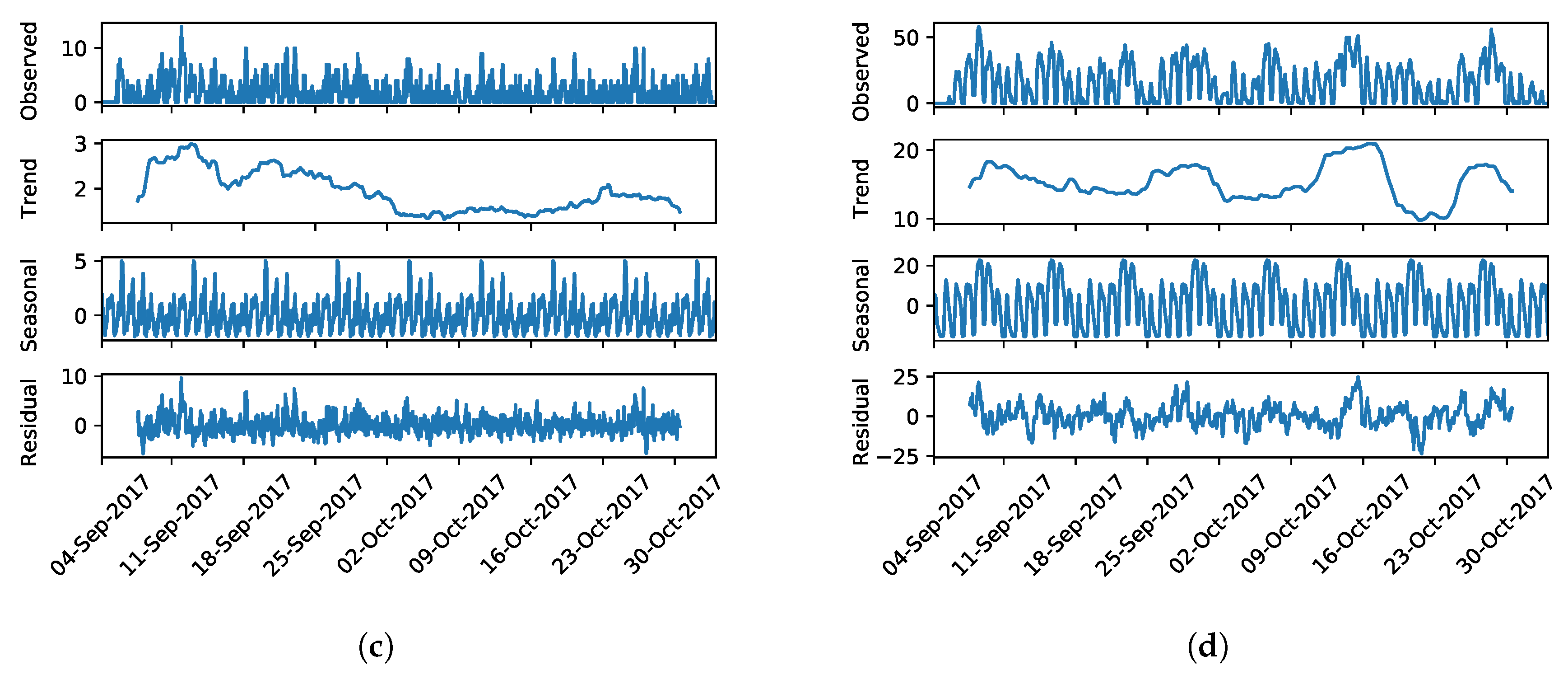
4.7. Evaluation of Time Series Stationarity

Considering the performance results, here we investigate the input data to understand the needs of ML-based solutions. For this, we decompose each occupation level time series in three main components [46]:

• trend: the low frequency changes, representing the non-stationarity long-term changes;
• seasonality: the periodic short-term repetition;
• residual: the noise evaluated as the remaining variation.

For the decomposition, we employ a moving average algorithm. Intuitively, the decomposition allow us to characterize each time series and better understand our problem for forecasting. Furthermore, it allows us to evaluate stationarity of the time series, hence the needs of ML-solutions rather than simpler solutions, e.g., AutoRegressive models or our baseline.

Figure 10 reports the observed occupation level of the representative cells along with their seasonal decomposition. Focusing on the business cell (Figure 10a), we can see how the observed cell occupation level vary from 0 up to 20 cars per time bin. Looking at the resulting components, we can see how the trend component accounts for only from one up to three cars in the entire period. This may suggest the stationarity of the time series as no major long-terms variation appear. However, looking at the seasonal and residual components, we can see how both have high and similar variations with residual having a range from −10 up to 10 occupation level. The latter being the noise component, it highlights how the time series is non-stationary. Focusing on the other cells, we can see how they lead to similar findings, hence highlighting the infeasibility of simple autoregressive solutions in favor of the ML-based solutions.

5. Discussion and Conclusions

This study presents a general-purpose framework to analyze historical FFCS usage data and to predict short-term car availability in restricted urban areas.

We showed the effectiveness and efficiency of the proposed framework on one among the biggest Free Floating Car Sharing services in Europe. The reported results show that the proposed framework can be used to accurately predict the occupancy level of the subareas of a smart city by means of contextualized models. Moreover, the proposed framework allowed us to analyze the spatial and temporal contextual conditions under which ML-based approaches are more accurate than simpler baseline approaches and which data models are more adequate depending on the context and the characteristics of the target cell.

The performed analyses and the results presented in Section 4 allow us to sketch a preliminary set of guidelines for operators who are interested in integrating a occupancy level prediction system in their service. The hints included in the guidelines try to balance the effect of complementary aspects such as (i) the accuracy of the prediction, (ii) the required time and memory for model generation, and (iii) cardinality of the knowledge base for building the prediction model.

Guidelines are summarized below:

• When should I use ML-based approaches? ML-based approaches are recommended when they achieve significantly more accurate performance than baseline techniques. This typically happens in the spatio-temporal situations that are characterized by non-stationary trends and, in particular, in all the cases in which the occupancy level is not a linear function of the input data (see Section 4.2) and only when the prediction horizon is more than 1 h (see Figure 6a).
• To what extent should I trust on baseline approaches? Baseline methods are comparable or slightly more accurate than ML-based approaches in (quasi-)stationary contexts, e.g., during the weekend in business cells (see Table 1 and Table 2). In these contexts, baseline methods are preferable because they achieve fairly low prediction errors spending less time in model training.
• On which data model should I rely on? Testing multiple data models is recommended since the best performing one is likely to change while considering different temporal, spatial, and functional contexts. For example, ML-based models for business cells during the morning should be trained using the Cell-Specific enriched with dynamic neighborhood data model because the occupancy levels of those cells are, on average, fairly correlated with faraway cells (see Table 3). Oppositely, predictors for isolated subareas (e.g., transport hub cells) should be trained by considering only the occupancy levels of the target cell (Cell-Specific data model) (see Table 6). In the latter case, the CS data model is more accurate yet simpler (in terms of data dimensionality), thus the computational time is more limited.
• Which regression algorithms should I integrate in the ML pipeline? Whenever the context requires the use of ML, the Random Forest regression algorithm turned out to be the most accurate model in dynamic contexts (e.g., in the weekdays) according to our preliminary experiments. However, the average MAE values achieved by different algorithms are, in many cases, comparable with each other. Hence, we recommend to perform multiple tests and to eventually ensemble model outcomes to get more reliable estimates (see Table 5).

As future work, we plan to extend the empirical study to different cities and countries and to enrich the current framework with further contextual metadata. For instance, the information about the average trip length, the refueling operations, the scheduled maintenance and car relocation activities could be used to enhance cell correlation analyses as well as to reduce the bias due to external, asynchronous actions of the service operators. Since the proposed framework is general-purpose, it can be profitably used to address the occupancy level prediction problem for various cities. Combining contextual data acquired in different cities is another interesting research direction. For example, the aggregated demographic profiles of the FFCS service users and the similarity between POIs located in different cities could also be exploited to enrich the current data models.