Article

One-Dimensional Convolutional Neural Networks with Feature Selection for Highly Concise Rule Extraction from Credit Scoring Datasets with Heterogeneous Attributes

Department of Computer Science, Meiji University, Kawasaki 214-8571, Japan
*
Author to whom correspondence should be addressed.
Electronics 2020, 9(8), 1318; https://doi.org/10.3390/electronics9081318
Submission received: 9 July 2020 / Revised: 8 August 2020 / Accepted: 14 August 2020 / Published: 16 August 2020

Abstract

:
Convolution neural networks (CNNs) have proven effectiveness, but they are not applicable to all datasets, such as those with heterogeneous attributes, which are often used in the finance and banking industries. Such datasets are difficult to classify, and to date, existing high-accuracy classifiers and rule-extraction methods have not been able to achieve sufficiently high classification accuracies or concise classification rules. This study aims to provide a new approach for achieving transparency and conciseness in credit scoring datasets with heterogeneous attributes by using a one-dimensional (1D) fully-connected layer first CNN combined with the Recursive-Rule Extraction (Re-RX) algorithm with a J48graft decision tree (hereafter 1D FCLF-CNN). Based on a comparison between the proposed 1D FCLF-CNN and existing rule extraction methods, our architecture enabled the extraction of the most concise rules (6.2) and achieved the best accuracy (73.10%), i.e., the highest interpretability–priority rule extraction. These results suggest that the 1D FCLF-CNN with Re-RX with J48graft is very effective for extracting highly concise rules for heterogeneous credit scoring datasets. Although it does not completely overcome the accuracy–interpretability dilemma for deep learning, it does appear to resolve this issue for credit scoring datasets with heterogeneous attributes, and thus, could lead to a new era in the financial industry.

1. Introduction

1.1. Background

Historically, assessing credit risk has been very important, yet extremely difficult. The banking industry faces numerous types of risk that affect not only banks but also customers. A key element of risk management in the banking industry is the need for appropriate customer selection. Credit scoring is an effective approach used by banks to analyze money borrowing and lending [1]. To manage financial risks, banks need to collect information from customers and other financial institutions to be able to make sound decisions in terms of whether to lend money to clients; to this end, collecting financial information can help differentiate safe from risky borrowers. Recently, the extraordinary increases in computing speed coupled with considerable theoretical advances in machine learning algorithms have created a renaissance in high modeling capabilities, with credit scoring being one of numerous examples. Indeed, with advanced modeling capabilities, researchers have achieved very high performances in making financial risk predictions [2].

1.2. Types of Data Attributes

Data attributes consist of two major classes: categorical and numerical. Categorical attributes are composed of two subclasses—nominal attributes and ordinal attributes—with the latter inheriting some properties of the former. Similar to nominal attributes, all of the categories (i.e., the possible values) of attributes in ordinal data—in other words, the data associated with only the ordinal attributes—are qualitative and, therefore, unsuitable for mathematical operations; however, they are naturally ordered and comparable [3].

1.3. Heterogeneous Credit Scoring

Credit scoring is a method used to assess the creditworthiness of a person or company applying for bank credit. The characteristics of the dataset differ from those of structured datasets that contain only ordinal attributes, such as the Australian credit scoring dataset (https://archive.ics.uci.edu/ml/datasets/Statlog+(Australian+credit+approval)). From a practical perspective, categorical data that involve a mix of nominal and ordinal attributes are common in credit scoring datasets [3]. In many cases, credit scoring datasets contain customer profiles that consist of numerical, ordinal, and mainly nominal attributes. Hereafter, we refer to these as heterogeneous credit scoring datasets. The German (-category) credit scoring dataset (https://archive.ics.uci.edu/ml/datasets/statlog+(German+credit+data)) is typical of heterogeneous credit scoring datasets. The heterogeneous (mixed attributes) structure of this dataset makes it difficult to achieve very high accuracy in terms of credit scoring. Therefore, a number of alternative approaches have been developed for credit scoring in the Australian and German datasets in recent years, including support vector machines (SVMs) [4], ensemble classifiers [5,6], feature selection [7], extreme learning machines [8], and deep learning (DL)-inspired classifiers [1,9].
Datasets that consist of heterogeneous attributes, such as the Australian and German datasets, contain both numerical (continuous) and categorical attributes. Some classification and rule extraction algorithms, such as SVMs and neural networks (NNs), do not work well with heterogeneous attributes because to convert categorical into continuous values, a unique integer is assigned to each categorical value in each feature set [10].

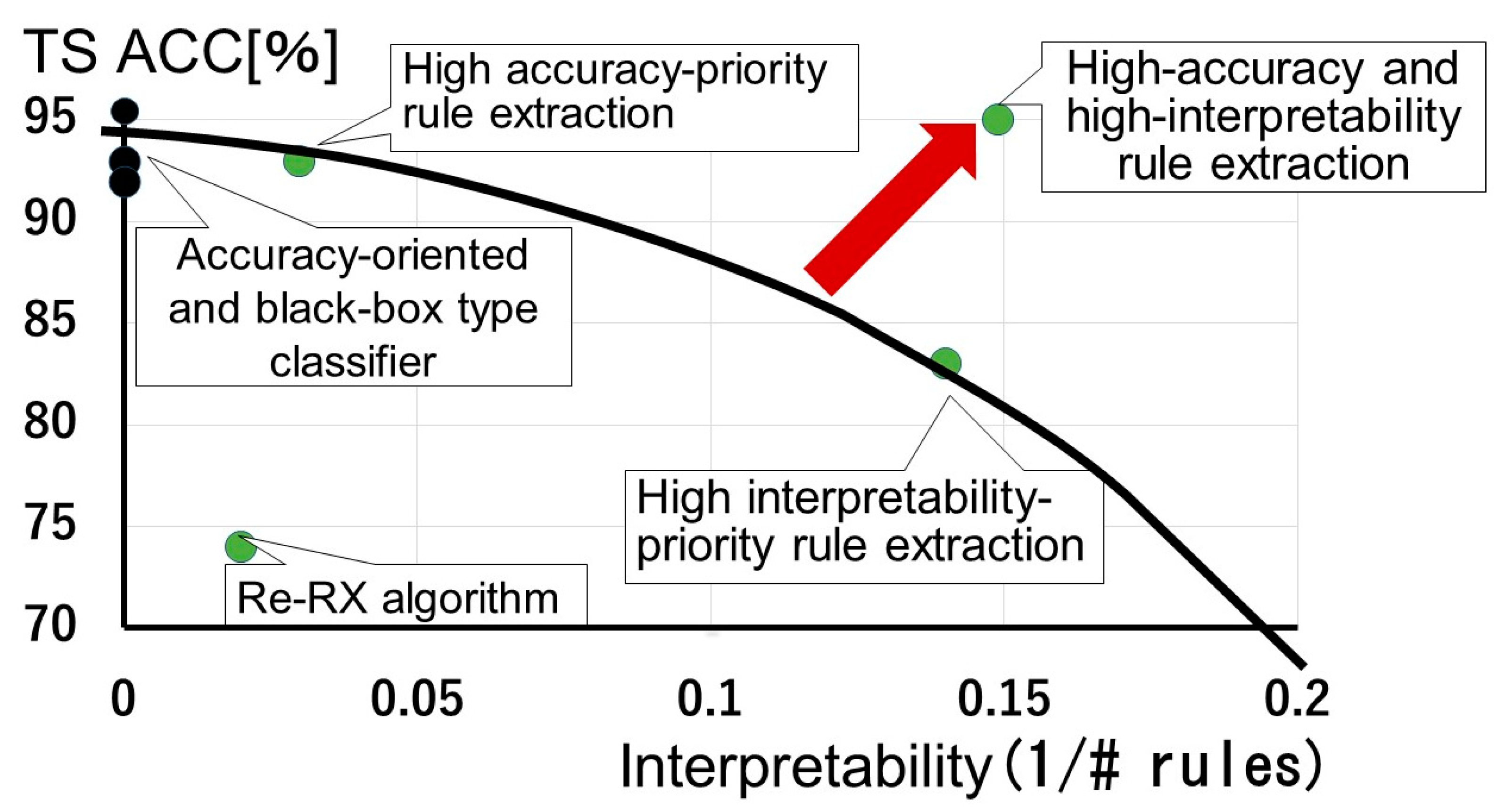
1.4. Accuracy–Interpretability Dilemma

In credit scoring, not only accuracy but also model interpretability is crucially important for three main reasons. First, bank managers require interpretable models to be able to justify any reason given for denying credit. Second, an interpretable model reduces the reluctance of bank managers to use statistical techniques for making credit-related decisions [11]. Third, bank managers gain insight into factors that affect credit only to the degree that they understand the information they receive [12].
Accuracy and interpretability have always been difficult to balance, and this is known as the accuracy–interpretability dilemma [13]. Although a variety of complicated predictive high-performance models have been proposed in the literature, in practice, interpretable models are still required by the financial industry [12,14,15].

1.5. Rule Extraction and the “Black Box” Problem

Rule extraction was originally proposed by Gallant [16] for a shallow NN and by Saito and Nakano [17] for the medical domain. For many years, extensive efforts have been made by many researchers to resolve the “black box” problem of trained NNs using rule extraction [18]. Rule extraction is a powerful type of artificial intelligence (AI)-based data mining that provides explanations and interpretable capabilities for models generated by shallow NNs. Rule extraction attempts to reconcile accuracy and interpretability by building a simple rule set that mimics how a well-performing complex model (i.e., a “black box”) makes decisions for users [19]. The present author [20] previously conducted a highly-cited survey on rule extraction algorithms and methods under a soft computing framework. Bologna [21] proposed a new technique to extract “if-then-else” rules from discretized interpretable multi-layer perceptron (DIMLP) ensembles, which was a pioneering work on rule extraction for NN ensembles. Setiono et al. [22] first proposed a unique algorithm for concise rule extraction using the concept of recursive-rule extraction. As a promising means to address the “black box” problem, a rule extraction technology that is well-balanced between accuracy and interpretability was proposed for shallow NNs [22]. Recently, Hayashi and Oisi [23] proposed a high-accuracy priority rule extraction algorithm to enhance both the accuracy and interpretability of extracted rules; this is realized by reconciling both of these criteria.
However, recently, a “new black box” problem caused by highly complex deep neural networks (DNNs) generated by DL has arisen. To resolve this “new black box” problem, transparency and interpretability are needed in DNNs. Symbolic rules were initially generated from deep belief networks (DBNs) by Tran and Garcez d’Avila [24], who trained a DBN using the MNIST dataset. The present author previously carried out a survey on the right direction needed to develop “white box” deep learning for medical images [25] and also provided new unified insights on deep learning for radiological and pathological images [26].

1.6. Recursive-Rule Extraction (Re-RX) and Related Algorithms

The Re-RX algorithm developed by Setiono et al. [22] repeats a backpropagation NN (BPNN), NN pruning [27], and a C4.5 decision tree (DT) [28] in a recursive manner. A major advantage of the Re-RX algorithm, which was designed as a rule extraction tool, is that it provides a hierarchical, recursive consideration of discrete variables prior to the analysis of continuous data. Additionally, it can generate classification rules from NNs that have been trained based on discrete and continuous attributes. We previously proposed Re-RX with J48graft [29] for improving the interpretability of extracted rules, Continuous Re-RX [30] for improving the accuracy of rule extraction, and Continuous Re-RX with J48graft [18] for high accuracy-priority rule extraction.

2. Motivation for This Work

Motivation for Research

Recently, DL has been applied in many fields because of its theoretical appeal and remarkable performance in terms of predictive accuracy. Despite comparisons with standard data mining algorithms that highlight the superiority of such tools, its application to credit scoring for datasets with heterogeneous attributes remains limited. Thus, it has become increasingly important to interpret “black boxes” in machine learning, particularly in regard to convolutional neural networks (CNNs), because of their lack of transparency. However, previous rule extraction methods are inappropriate for CNNs, largely because they cannot generate concise and interpretable rules [25].
Explanations are particularly relevant in the banking sector, so “black box” models are approached with caution. Actually, banking managers are typically unwilling to use DL for credit scoring when credit is denied to a customer.
As shown in Figure 1, the best trade-off is when accuracy and interpretability can be enhanced simultaneously. The black line indicates the trade-off curve (Pareto optimal), which balances accuracy and interpretability. The red arrow indicates a shift from the trade-off curve to the ideal point (high-accuracy and high-interpretability; most concise). We previously proposed a method to achieve high accuracy-priority rule extraction [18]. “Black box” classifiers can be plotted as black dots placed vertically on the axis for the test dataset accuracy (TS ACC). These accuracies are often higher than those obtained using high accuracy-priority rule extraction for credit scoring datasets, which indicates that the latest high-performance classifier for the Australian dataset does not completely overcome the accuracy–interpretability dilemma [10]. In this section, as Re-RX with J48graft is the most important component of our proposed method, we depict it using mathematical notations in Figure 2.
The highest accuracy achieved for the German (-categorical) dataset was 86.57% by Tripathi et al. [7]. Kuppili et al. [8] and Tripathi et al. [9] achieved considerably higher accuracies using an SVM and NN requiring that each data instance was represented as a vector of real numbers. However, they did not handle nominal attributes appropriately as they converted these into numerical attributes before feeding them into classifiers. To handle datasets with heterogeneous attributes appropriately and maintain the characteristics of the nominal attributes, we believe that no such conversion should be conducted. For example, as follows, we show descriptions of three attributes of the German dataset:
Attribute 1: (category—ordinal)
Status of existing checking account
A11: … < 0 DM (Deutsche Mark)
A12: 0 ≤ … < 200 DM
A13: … ≥ 200 DM/salary assignments for at least 1 year
Attribute 2: (continuous, numerical)
Duration in months
Attribute 3: (category—nominal)
Credit history
A30: no credit taken/all credits paid back duly
A31: all credits at this bank paid back duly
A32: existing credits paid back duly until now
A33: delay in paying off in the past
A34: critical account/other credits existing (not at this bank)
Despite the effectiveness of CNNs, researchers tend to overlook three issues; they are only applicable to: (1) datasets with rich information hidden in the data, as in computer vision; (2) structured datasets consisting of ordinal attributes; and (3) feature extraction from images. Resolving these issues could expand the utility of CNNs to interpretable AI for wider and practical applications in finance and banking. Therefore, this study aims to provide a new approach for transparency and conciseness in heterogeneous attribute datasets using a one-dimensional (1D) CNN and the Re-RX algorithm with J48graft.
Table 1 highlights our motivation. The advantage of our proposed method is that it provides transparency and conciseness for datasets with heterogeneous attributes, whereas the disadvantage is that it achieves slightly lower classification accuracy.
In the following section, we describe the Re-RX algorithm, Re-RX with J48graft, and 1D fully-connected layer first CNN (1D FCLF-CNN). In Section 4, we propose highly concise rule extraction using the 1D FCLF-CNN with Re-RX with J48graft. In Section 5, we describe experiments involving two credit scoring datasets. In Section 6, we present the results based on the performance of our and existing rule extraction methods. In Section 7, we discuss the significance of the 1D FCLF-CNN with Re-RX with J48graft in terms of transparency and conciseness in heterogeneous credit scoring. Finally, in Section 8, we summarize our findings.

3. Methods

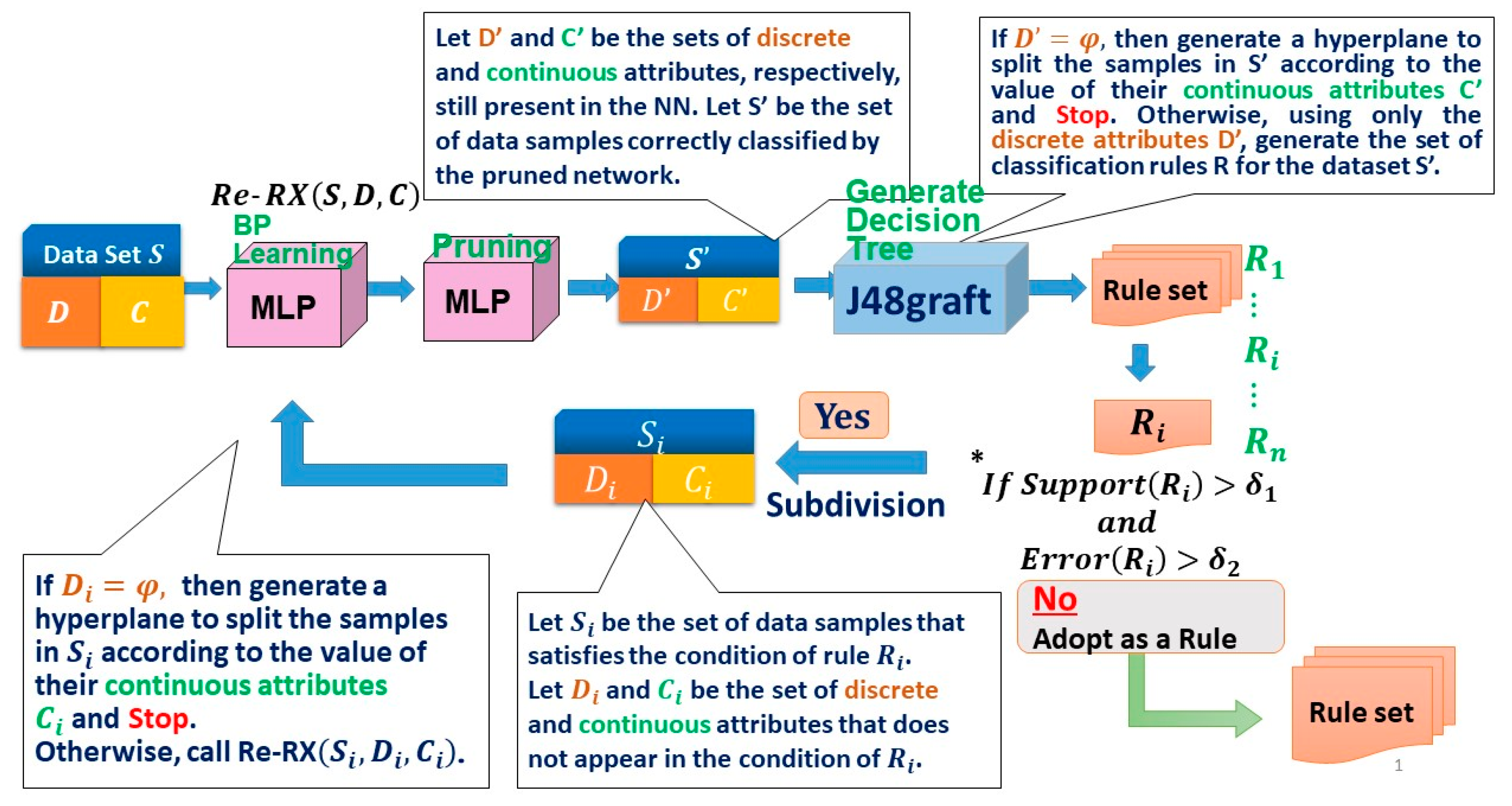
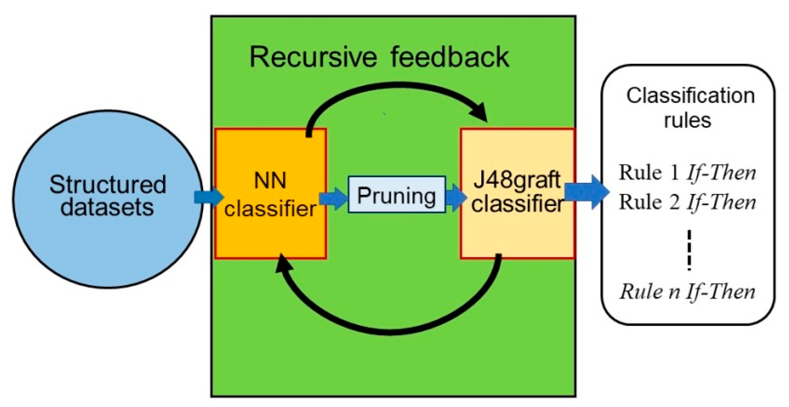
3.1. Re-RX Algorithm with J48graft

To achieve both highly concise and accurate extracted rules, we recently proposed Re-RX with J48graft [29,31], which is a “white box” model capable of providing highly accurate and concise classification rules. As the potential capabilities of Re-RX with J48graft are somewhat unclear in regard to extracting highly accurate and concise classification rules, we decided to elucidate the synergistic effects between grafting and subdivision, which work effectively in combination. For a better understanding of the mechanism underlying Re-RX with J48graft, a schematic overview is provided in Figure 2.
As shown in Figure 3, a credit scoring dataset with all attributes was fed into a BPNN using a BP classifier and pruned to remove irrelevant and redundant attributes. Next, a DT was generated using J48graft [32] (grafted C4.5, i.e., C4.5A [33]).
We also created if-then rules from the DT using postprocessing of J48graft. Each rule generated using J48graft was not satisfactory for the given criterion, so the rule was further subdivided (i.e., classification accuracy was enhanced, while the number of attributes per extracted rule and rules per rule set increased) by the Re-RX algorithm.
We defined support for a rule as being based on the percentage of samples covered by that rule. The support and corresponding error (incorrectly classified) rate of each rule were then checked. If the error exceeded the covering rate while the support met the minimum threshold, then the rule was further subdivided by calling the Re-RX algorithm recursively.
In contrast to existing “black box” models, Re-RX with J48graft provides high classification accuracy and can be easily explained and interpreted in terms of concise extracted rules; that is, Re-RX with J48graft is a “white box” (more understandable) model.

3.2. Deep Convolutional Neural Networks (DCNNs) and Inception Modules

DCNNs consist of a large number of connected NN convolutional or pooling layers. In addition, DCNN structures have many overlapping layers; this increases the size of the features, including the fully connected layers. Krizhevsky et al. [34] proposed AlexNet, which has achieved remarkably improved performance, and this success has attracted much attention in DCNNs. Simonyan and Zisserman [35] proposed VGGNet, which consists of 19 layers, and is therefore deeper than AlexNet. VGGNet uses a 3 × 3 sized filter to extract more complex and representative features. VGGNet can better approximate the objective function with increased nonlinearity and obtain a better feature representation as the depth of the layer increases. However, DCNNs such as VGGNet are faced with a number of problems, including degradation and high computational requirements in terms of both memory and time.
Szegedy et al. [36] proposed GoogLeNet, a deeper and wider network than previous architectures. In GoogLeNet, a new module called inception, which is a combination of layers with concatenated convolution filters, was introduced. Inception modules [36] are basically stacked on top of each other to comprise a network. The main idea was to consider a sparse structure in the CNN architecture and cover the available dense components [37].

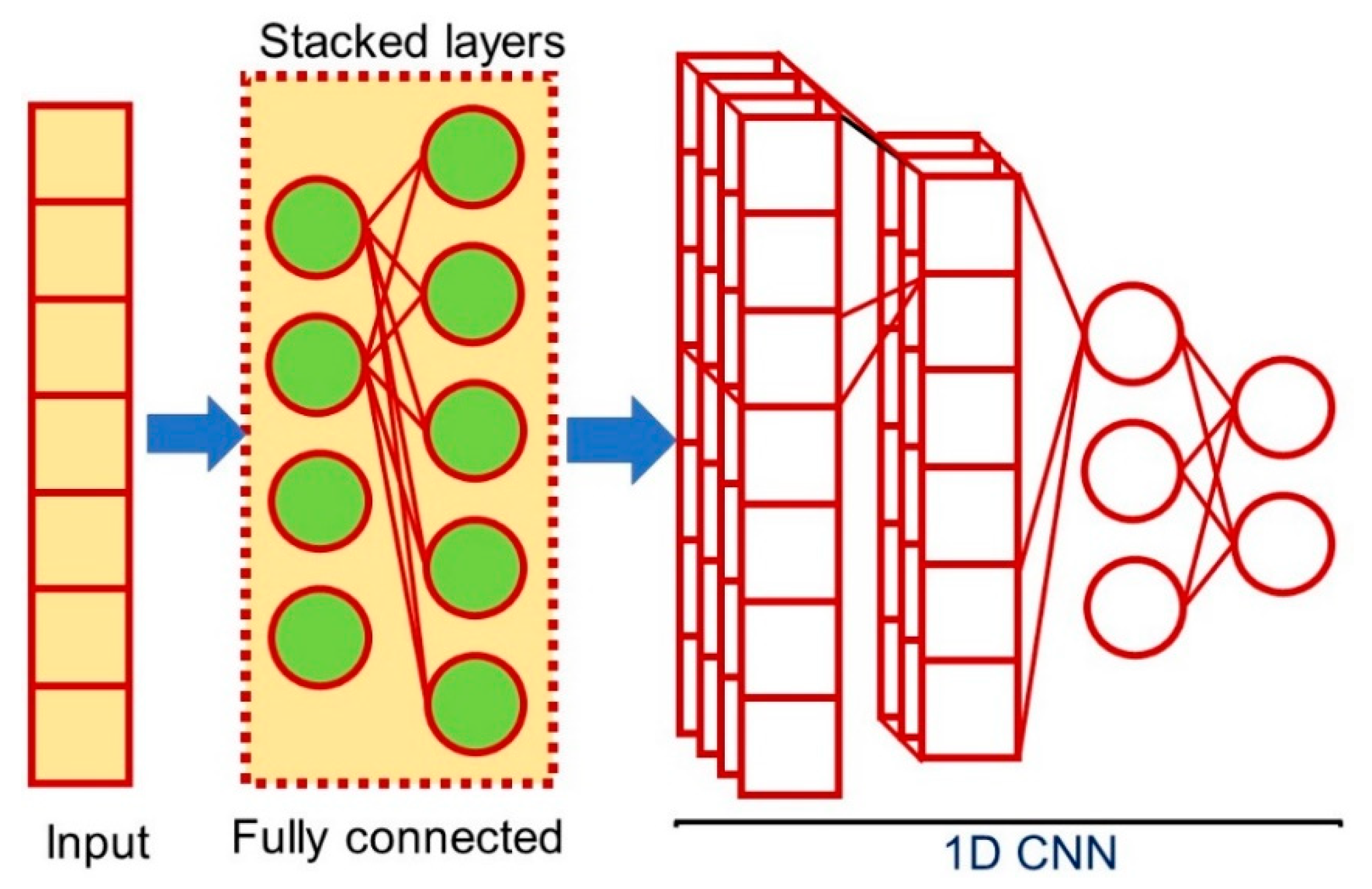
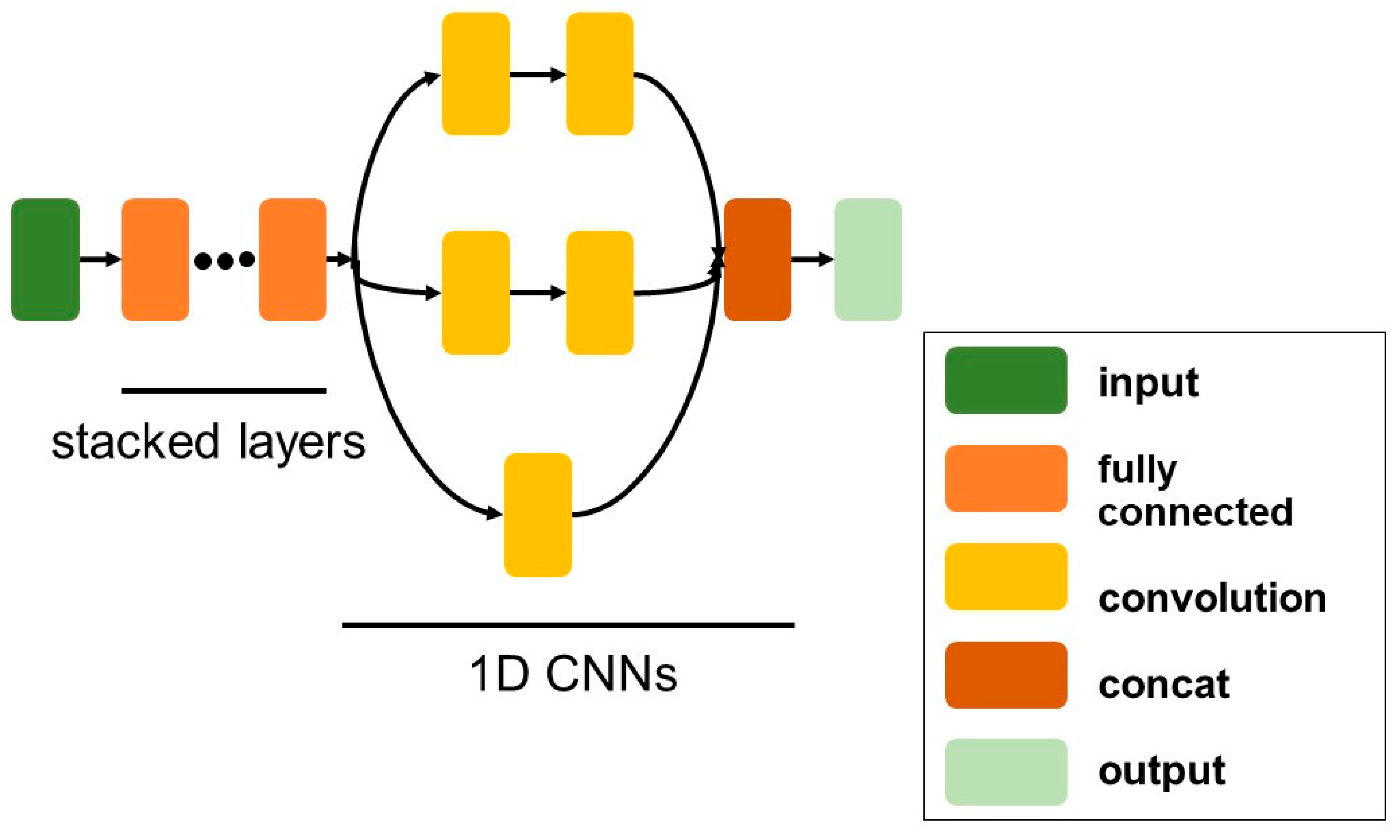
3.3. One-Dimensional Fully-Connected Layer First CNN (1D FCLF-CNN)

Liu et al. [38] first proposed a 1D FCLF-CNN to improve the classification performance of structured datasets. In this network, the input layer is first connected to several fully connected layers, followed by a typical CNN. Structured datasets are similar to disrupted image data, which appear to have no local structure. In the 1D FCLF-CNN, the fully-connected layers before the convolutional layers are seen as an encoder. Liu et al. [38] also used a fully-connected layer as an encoder by adding a Softmax layer, which normalizes the output of fully-connected layers to 0–1, where 0 means that the degree of confidence is the lowest, and 1 the highest, thereby providing an important degree of confidence for classification [39]. The encoder could transfer raw instances into representations with a better local structure. Therefore, they believed that a 1D FCLF-CNN using a fully-connected layer as an encoder would offer better performance than a pure 1D CNN. Thus, 1D FCLF-CNNs represent an encoder-CNN stacking method capable of providing better performance than pure CNNs, particularly for structured data.
For the convolutional layers of the 1D CNN and 1D FCLF-CNN, Liu et al. used variants of the inception module [40], i.e., a bank of filters with different filter sizes. The inception module was used because of its computational efficiency, and Keras [41] was implemented to build the 1D FCLF-CNN.

4. Theory

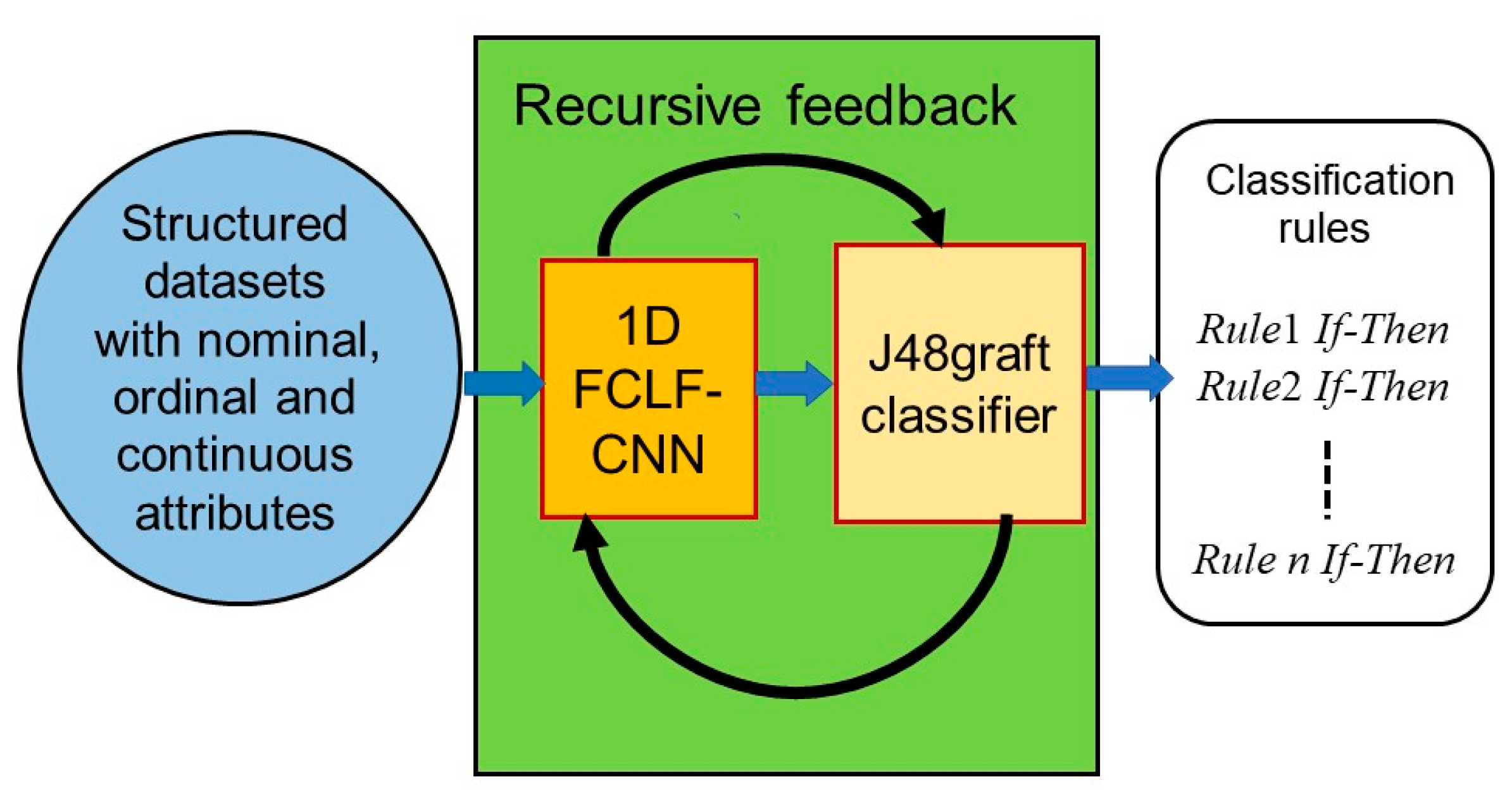
4.1. Highly Concise Rule Extraction Using a 1D FCLF-CNN with Re-RX with J48graft

As shown in Figure 2, Re-RX with J48graft consists of an NN and a J48graft classifier [18]. The Re-RX algorithm [22] does not make any assumptions regarding the NN architecture or pruning method. Thus, the NN classifier was replaced with a 1D FCLF-CNN (Figure 4) to improve the accuracy and drastically reduce the input features. We constructed a 1D FCLF-CNN using the inception module shown in Figure 5.
Next, Re-RX with J48graft was applied to extract highly concise rules for datasets consisting of heterogeneous attributes (nominal, categorical, and numerical attributes). The 1D FCLF-CNN with Re-RX with J48graft (Figure 6) achieved highly concise rule extraction.

4.2. Rationale Behind the Architecture for the 1D FCLF-CNN with Re-RX with J48graft

The proposed architecture can be applied to heterogeneous credit datasets because the Re-RX algorithm uses the J48graft DT. In the present method, the 1D FCLF-CNN provides selected attributes for inputs via dimensionality reduction, which enables Re-RX with J48graft to extract highly concise rules. Generally, rules can be extracted using pedagogical [19] approaches, such as C4.5 [28], J48graft [29,32], Trepan [42], and ALPA [24], regardless of the input and output layers of DL networks for structured datasets [25]. However, the proposed method can extract highly concise rules more effectively.

4.3. Attribute Selection by Dimension Reduction Using a 1D FCLF-CNN for Datasets with Heterogeneous Attributes

The advantages of inception include feature extraction, dimensionality reduction, and computational complexity reduction [37]. Therefore, variants of inception were used as the convolutional layers in the 1D CNN and 1D FCLF-CNN [38]. The 1D FCLF-CNN offers better classification performance because it detects more complex relations and reduces the number of input attributes for structured datasets. Additionally, it facilitates the classification process by separating a structured dataset belonging to different classes.
In this study, the 1D FCLF-CNN functioned as a classifier with high accuracy by eliminating unnecessary attributes. The number of attributes input in Re-RX with J48graft were considerably decreased. As a result, Re-RX with J48graft extracted drastically reduced numbers (−66.6%) of attributes compared with those obtained by Chakraborty et al. [43]. We can easily set the values for the covering and error rates in Re-RX with J48graft to minimize the number of subdivisions.

5. Experimental Procedure

In this study, k-fold cross-validation (CV) [44] was used to evaluate the classification rule accuracy of the test datasets and guarantee the validity of the results. Structured datasets were trained using the 1D FCLF-CNN with Re-RX with J48graft. Then, the average classification accuracy using 10CV for the test dataset (TS ACC), the number of extracted rules (# rules), and the area under the receiver operating characteristic curve (AUC-ROC) [45] were obtained for the test dataset. The 1D FCLF-CNN with Re-RX with J48graft took approximately 160 and 270 s to train the German and Australian datasets, respectively, on a conventional PC (Intel Core i7 7500U; 2.7 GHz Intel; 8 GB RAM). The testing time was negligible. In this study, Keras was used with Python for the German and Australian datasets. We used ReLU and tanh as activation functions for the Australian and German datasets, respectively. We used Tree-structured Parzen Estimators (TPEs) [46] to optimize the hyperparameter values shown in Table 2. We also used TPEs to optimize the type of activation functions because they optimize discrete functions to determine the type of functions. The numbers of layers in the inception module and the structure are shown in Figure 5.
In previous works, the German dataset has been considered to have 13 categorical attributes; however, based on the purposes of these attributes, 11 of them should in fact be treated as nominal attributes, as shown in Table 3.

6. Results

A comparison of the TS ACC and the average number of extracted rules (conciseness) for the German dataset is shown in Table 4 and Table 5, respectively. Similarly, a comparison of the TS ACC and the average number of extracted rules (conciseness) for the Australian dataset is shown in Table 6 and Table 7, respectively. Here, the parameters in Table 2 were used.
An example rule set for the German dataset (73.0% TS ACC) extracted by the proposed architecture is presented below:
Rule 1: IF A1 = 1 AND A3 ≤ 2 THEN Class 1
Rule 2: IF A1 = 1 AND A3 > 2 THEN Class 0
Rule 3: IF A1 = 2 AND A12 = 4 THEN Class 1
Rule 4: IF A1 = 2 AND A12 ≠ 4 THEN Class 0
Rule 5: IF A1 ≥ 3 THEN Class 0
where Class 0 is a good payer; Class 1 is a bad payer; A1 is the status of an existing checking account; A1 = 1 is <0 DM—no checking account; A1 = 2 is <200 DM; A1 > 3 is ≥200 DM/salary assignments; A3 is credit history; A3 = 1 is all credit at this bank paid back duly; A3 = 2 is existing credits paid back duly until now; A3 = 3 is the delay in paying off debt in the past; A12 is property; and A12 = 4 is unknown/no property.
An example rule set for the Australian dataset (87.14% TS ACC) extracted by the proposed architecture is presented below.
Rule 1: IF A8=0 THEN Class 0.
Rule 2: IF A8=1 AND A9=0 THEN Class 0.
Rule 3: IF A8=1 AND A9 =1 THEN Class 1.

7. Discussion

7.1. Discussion

The highest classification accuracy achieved for the German dataset (86.57%; [7]) was considerably lower than that for the Australian dataset [9], which suggests that the German dataset was more difficult to classify. The accuracy–interpretability dilemma often needs to be overcome based on the performance obtained using interpretability–priority rule extraction, which is an accuracy-oriented and “black box”-type classifier. Even if DL-inspired techniques are effective in improving the classification accuracy, these methods could not be expected to transform the “black box” nature of DNNs trained using DL into a “white box” nature consisting of a series of interpretable classification rules.
We demonstrated a trade-off between the average accuracy and number of extracted rules in previous rule extraction methods [18]. As we previously described [31], when comparing rule sets before and after subdivision, accuracy is expected to increase if a rule set has a higher average number of antecedents; however, the higher the number of antecedents, the more complex the extracted rules. In this case, not only decreased interpretability but also decreased generalization capability and overfitting were observed for the test dataset.
Although Hayashi and Oisi [18] achieved the highest accuracy reported, their number of extracted rules was 44.9, and a trade-off was apparent between accuracy and interpretability (reciprocal of the number of rules) for high accuracy-priority rule extraction. By contrast, Setiono et al. [53] proposed MINERVA, which achieved lower accuracy (70.51%) and extracted 8.4 concise rules for high interpretability–priority rule extraction.
Recently, Santana et al. [54] reported classification rules for the German dataset using an NN with a self-organization map (SOM) [55] and particle swarm optimization (PSO) [56]. The average number of rules was 6.344 and the precision was 0.69. However, the number of rules to classify was slightly larger, and the precision was inferior compared with that in the present study (73.10%). Very recently, Chakraborty et al. [43] proposed rule extraction from a DNN using a deep belief network and BP (ERENN-MHL). They achieved a TS ACC of 74.50% and an average number of 8.0 rules using 5CV for the German dataset.
In this paper, we achieved the most concise rules (6.2) and the best accuracy (73.10%), i.e., the highest interpretability–priority rule extraction, for credit scoring datasets with heterogeneous attributes. Re-RX with J48graft achieved slightly lower accuracy (72.78%) and extracted many more rules (16.65) [18], which were the fewest for this level of accuracy. However, in terms of accuracy or interpretability, no further major developments were achieved.
To solve the dilemma for datasets with heterogeneous attributes, the 1D FCLF-CNN with Re-RX with J48graft functioned as a high-accuracy classifier by eliminating unnecessary attributes, which drastically reduced the number of extracted rules. Therefore, the proposed method provided the most concise rules (see Table 4).
For the Australian dataset, the 1D FCLF-CNN with Re-RX with J48graft achieved the most concise rules (2.6) and considerably lower accuracy (86.53%) than the highest accuracy classifier (97.39%). However, unlike the German dataset, the Australian dataset contains no nominal attributes; hence, it can be easily handled by DL-inspired classifiers [10]. Furthermore, the proposed algorithm achieved a slightly lower accuracy than the DL-based method [52].
On the other hand, Santana et al. (2017) reported classification rules for the Australian dataset using an NN with an SOM and PSO. The average number of rules was 3.01, and the precision was 0.858. Although, the number of classification rules was substantially larger, the precision was inferior to that achieved in the present study (86.53%). These results suggest that the proposed 1D FCLF-CNN with Re-RX with J48graft is very effective for extracting highly concise rules for heterogeneous credit datasets.

7.2. Common Issues with Re-RX with J48graft and ERENN-MHL

Both Re-RX with J48graft and ERENN-MHL use the support (covering) and error rates to reconcile accuracy and interpretability. Chakraborty et al. achieved a TS ACC of 74.50% and 8.0 rules for the German dataset. These rates were quite sensitive in terms of balancing accuracy and interpretability [22,43]. Chakraborty et al. used 12 and 5 attributes for the German and Australian datasets, respectively, to achieve average numbers of 1.6 and 1.0 antecedents (attributes per rule), respectively. By contrast, our proposed method achieved average numbers of 1.24 and 0.86 antecedents for the German and Australian datasets, respectively. Therefore, our method achieved substantially more conciseness than ERENN-MHL.
Regarding the German dataset, attributes A1 and A3 were identical to the selected attributes according to all six feature selection approaches [7], whereas A12 was selected by three feature selection approaches. For the Australian dataset, A8 was identical to the selected attributes according to all feature selection approaches, whereas A9 was selected by five feature-selection approaches. Furthermore, the number of rules in the German and Australian datasets drastically decreased to 6.2 and 2.6, respectively. These results suggest that the dimension reduction in the 1D FCLF-CNN was extremely effective in terms of feature selection for Re-RX with J48graft and enabled highly concise rule extraction.
In summary, the main contribution of this study is the proposal of a 1D FCLF-CNN with Re-RX with J48graft. We believe that by eliminating unnecessary attributes, this method enables highly accurate classification, and as a result, Re-RX with J48graft avoids the disadvantages described in Section 3.1 and can extract highly concise rules for heterogeneous credit scoring datasets effectively.

8. Conclusions

Datasets with heterogeneous attributes are often used in the finance and banking industries. However, such datasets (e.g., the German dataset) are difficult to classify, and to date, existing high-accuracy classifiers and rule-extraction methods have not been able to achieve sufficiently high classification accuracies or concise classification rules. In this study, a 1D FCLF-CNN with Re-RX with J48graft was proposed to extract highly concise rules for credit scoring datasets with heterogeneous attributes. Although the 1D FCLF-CNN with Re-RX with J48graft does not completely overcome the accuracy–interpretability dilemma for DL, it does appear to resolve this issue for credit scoring datasets with heterogeneous attributes. Therefore, the proposed method could lead to a new era in the financial industry.

Author Contributions

Conceptualization, Y.H.; methodology, Y.H., N.T.; software, N.T.; validation, Y.H.; investigation, Y.H.; resources, Y.H.; data curation, Y.H.; writing—original draft preparation, Y.H.; writing—review and editing, Y.H.; visualization, Y.H., N.T.; supervision, Y.H.; funding acquisition, Y.H. All authors have read and agreed to the published version of the manuscript.

Funding

This work was supported in part by the Japan Society for the Promotion of Science through a Grant-in-Aid for Scientific Research (C) (No. 18K11481).

Conflicts of Interest

The authors declare no conflict of interest.

Notations

1/#Reciprocal number
TS ACCTest accuracy
# rulesNumber of rules
10 × 10CV10 runs of 10-fold cross-validation

Abbreviations

CNNConvolutional neural network
1DOne-dimensional
FCLFFully-connected layer first
Re-RXRecursive-rule eXtraction
SVMSupport vector machine
DLDeep learning
NNNeural network
DNNDeep neural network
AIArtificial intelligence
DCNNDeep convolutional neural network
BPNNBackpropagation neural network
CVCross-validation
AUC-ROCArea under the receiver operating characteristic curve
SMOTESynthetic minority over-sampling technique
DMDeutsche Mark
SOMSelf-organization map
PSOParticle swarm optimization
ERENN-MHLElectric rule extraction from a neural network with a multi-hidden layer for a DNN

References

  1. Pławiak, P.; Abdar, M.; Pławiak, J.; Makarenkov, V.; Acharya, U.R. DGHNL: A new deep genetic hierarchical network of learners for prediction of credit scoring. Inf. Sci. 2020, 516, 401–418. [Google Scholar] [CrossRef]
  2. Liberati, C.; Camillo, F.; Saporta, G. Advances in credit scoring: Combining performance and interpretation in kernel discriminant analysis. Adv. Data Anal. Classif. 2015, 11, 121–138. [Google Scholar] [CrossRef]
  3. Zhang, Y.; Cheung, Y.-M.; Tan, K.C. A Unified Entropy-Based Distance Metric for Ordinal-and-Nominal-Attribute Data Clustering. IEEE Trans. Neural Netw. Learn. Syst. 2020, 31, 39–52. [Google Scholar] [CrossRef] [PubMed]
  4. Martens, D.; Baesens, B.; Van Gestel, T.; Vanthienen, J. Comprehensible credit scoring models using rule extraction from support vector machines. Eur. J. Oper. Res. 2007, 183, 1466–1476. [Google Scholar] [CrossRef]
  5. Abellán, J.; Mantas, C.J. Improving experimental studies about ensembles of classifiers for bankruptcy prediction and credit scoring. Expert Syst. Appl. 2014, 41, 3825–3830. [Google Scholar] [CrossRef]
  6. Abellán, J.; Castellano, J.G. A comparative study on base classifiers in ensemble methods for credit scoring. Expert Syst. Appl. 2017, 73, 1–10. [Google Scholar] [CrossRef]
  7. Tripathi, D.; Edla, D.R.; Cheruku, R. Hybrid credit scoring model using neighborhood rough set and multi-layer ensemble classification. J. Intell. Fuzzy Syst. 2018, 34, 1543–1549. [Google Scholar] [CrossRef]
  8. Kuppili, V.; Tripathi, D.; Edla, D.R. Credit score classification using spiking extreme learning machine. Comput. Intell. 2020, 36, 402–426. [Google Scholar] [CrossRef]
  9. Pławiak, P.; Abdar, M.; Acharya, U.R. Application of new deep genetic cascade ensemble of SVM classifiers to predict the Australian credit scoring. Appl. Soft Comput. 2019, 84, 105740. [Google Scholar] [CrossRef]
  10. Tripathi, D.; Edla, D.R.; Cheruku, R.; Kuppili, V. A novel hybrid credit scoring model based on ensemble feature selection and multilayer ensemble classification. Comput. Intell. 2019, 35, 371–394. [Google Scholar] [CrossRef]
  11. Sun, J.; Li, H.; Huang, Q.-H.; He, K.-Y. Predicting financial distress and corporate failure: A review from the state-of-the-art definitions, modeling, sampling, and featuring approaches. Knowl. Based Syst. 2014, 57, 41–56. [Google Scholar] [CrossRef]
  12. Chen, T.-C.; Cheng, C.-H. Hybrid models based on rough set classifiers for setting credit rating decision rules in the global banking industry. Knowl. Based Syst. 2013, 39, 224–239. [Google Scholar] [CrossRef]
  13. Florez-Lopez, R.; Ramon-Jeronimo, J.M. Enhancing accuracy and interpretability of ensemble strategies in credit risk assessment. A correlated-adjusted decision forest proposal. Expert Syst. Appl. 2015, 42, 5737–5753. [Google Scholar] [CrossRef]
  14. Mues, C.; Baesens, B.; Files, C.M.; Vanthienen, J. Decision diagrams in machine learning: An empirical study on real-life credit-risk data. Expert Syst. Appl. 2004, 27, 257–264. [Google Scholar] [CrossRef]
  15. Hsieh, N.-C.; Hung, L.-P. A data driven ensemble classifier for credit scoring analysis. Expert Syst. Appl. 2010, 37, 534–545. [Google Scholar] [CrossRef]
  16. Gallant, S.I. Connectionist expert systems. Commun. ACM 1988, 31, 152–169. [Google Scholar] [CrossRef]
  17. Saito, K.; Nakano, R. Medical Diagnosis Expert Systems Based on PDP Model. In Proceedings of the IEEE Interenational Conference Neural Network, San Diego, CA, USA, 1988, 24–27 July 1988; pp. I.255–I.262. [Google Scholar]
  18. Hayashi, Y.; Oishi, T. High Accuracy-priority Rule Extraction for Reconciling Accuracy and Interpretability in Credit Scoring. New Gener. Comput. 2018, 36, 393–418. [Google Scholar] [CrossRef]
  19. Andrews, R.; Diederich, J.; Tickle, A.B. Survey and critique of techniques for extracting rules from trained artificial neural networks. Knowl. Based Syst. 1995, 8, 373–389. [Google Scholar] [CrossRef]
  20. Mitra, S.; Hayashi, Y. Neuro-fuzzy rule generation: Survey in soft computing framework. IEEE Trans. Neural Netw. 2000, 11, 748–768. [Google Scholar] [CrossRef] [Green Version]
  21. Bologna, G. A study on rule extraction from several combined neural networks. Int. J. Neural Syst. 2001, 11, 247–255. [Google Scholar] [CrossRef]
  22. Setiono, R.; Baesens, B.; Mues, C. Recursive Neural Network Rule Extraction for Data with Mixed Attributes. IEEE Trans. Neural Netw. 2008, 19, 299–307. [Google Scholar] [CrossRef] [PubMed]
  23. Tran, S.N.; Garcez, A.S.D. Deep Logic Networks: Inserting and Extracting Knowledge from Deep Belief Networks. IEEE Trans. Neural Netw. Learn. Syst. 2016, 29, 246–258. [Google Scholar] [CrossRef]
  24. De Fortuny, E.J.; Martens, D. Active Learning-Based Pedagogical Rule Extraction. IEEE Trans. Neural Netw. Learn. Syst. 2015, 26, 2664–2677. [Google Scholar] [CrossRef] [PubMed] [Green Version]
  25. Hayashi, Y. The Right Direction Needed to Develop White-Box Deep Learning in Radiology, Pathology, and Ophthalmology: A Short Review. Front. Robot. AI 2019, 6, 1–8. [Google Scholar] [CrossRef]
  26. Hayashi, Y. New unified insights on deep learning in radiological and pathological images: Beyond quantitative performances to qualitative interpretation. Inform. Med. Unlocked 2020, 19, 100329. [Google Scholar] [CrossRef]
  27. Setiono, R. A Penalty-Function Approach for Pruning Feedforward Neural Networks. Neural Comput. 1997, 9, 185–204. [Google Scholar] [CrossRef]
  28. Quinlan, J.R. Programs for Machine Learning; Morgan Kaufman: San Mateo, CA, USA, 1993. [Google Scholar]
  29. Hayashi, Y.; Nakano, S. Use of a Recursive-Rule Extraction algorithm with J48graft to archive highly accurate and concise rule extraction from a large breast cancer dataset. Inform. Med. Unlocked 2015, 1, 9–16. [Google Scholar] [CrossRef] [Green Version]
  30. Hayashi, Y.; Nakano, S.; Fujisawa, S. Use of the recursive-rule extraction algorithm with continuous attributes to improve diagnostic accuracy in thyroid disease. Inform. Med. Unlocked 2015, 1, 1–8. [Google Scholar] [CrossRef] [Green Version]
  31. Hayashi, Y. Synergy effects between grafting and subdivision in Re-RX with J48graft for the diagnosis of thyroid disease. Knowl. Based Syst. 2017, 131, 170–182. [Google Scholar] [CrossRef]
  32. Witten, I.H.; Frank, E.; Hall, M.A. Data Mining: Practical Machine Learning Tools and Techniques; Elsevier BV: Amsterdam, The Netherlands, 2011. [Google Scholar]
  33. Webb, G.I. Decision Tree Grafting from the All-Tests-But-One Partition. In Proceedings of the 16th International Joint Conference on Artificial Intelligence, San Mateo, CA, USA, 10–16 July 1999; pp. 702–707. [Google Scholar]
  34. Krizhevsky, A.; Sutskever, I.; Hinton, G.E. lmageNet classification with deep convolutional neural networks. In Proceedings of the Advances in Neural Information Processing Systems, Lake Tahoe, NV, USA, 3–6 December 2012; pp. 1097–1105. [Google Scholar]
  35. Simonyan, K.; Zisserman, A. Very deep convolutional networks for large-scale image recognition. arXiv 2014, arXiv:1409.1556. [Google Scholar]
  36. Szegedy, C.; Liu, W.; Jia, Y.; Sermanet, P.; Reed, S.; Anguelov, D.; Erhan, D.; Vanhoucke, V.; Rabinovich, A. Going Deeper with Convolutions. In Proceedings of the 2015 IEEE Conference on Computer Vision and Pattern Recognition (CVPR), Boston, MA, USA, 7–12 June 2015; pp. 1–9. [Google Scholar]
  37. Kim, J.-Y.; Cho, S.-B. Exploiting deep convolutional neural networks for a neural-based learning classifier system. Neurocomputing 2019, 354, 61–70. [Google Scholar] [CrossRef]
  38. Liu, K.; Kang, G.; Zhang, N.; Hou, B. Breast Cancer Classification Based on Fully-Connected Layer First Convolutional Neural Networks. IEEE Access 2018, 6, 23722–23732. [Google Scholar] [CrossRef]
  39. Chen, C.; Jiang, F.; Yang, C.; Rho, S.; Shen, W.; Liu, S.; Liu, Z. Hyperspectral classification based on spectral–spatial convolutional neural networks. Eng. Appl. Artif. Intell. 2018, 68, 165–171. [Google Scholar] [CrossRef]
  40. Szegedy, C.; Vanhoucke, V.; Ioffe, S.; Shlens, J.; Wojna, Z. Rethinking the Inception Architecture for Computer Vision. In Proceedings of the 2016 IEEE Conference on Computer Vision and Pattern Recognition (CVPR), Las Vegas, NV, USA, 27–30 June 2016; pp. 2818–2826. [Google Scholar]
  41. Keras. Available online: https://github.com/keras-team/keras (accessed on 30 June 2020).
  42. Craven, J.M.; Shavlik, J. Extracting tree-structured representations of trained networks. Adv. Neural Inf. Process. Syst. 1996, 8, 24–30. [Google Scholar]
  43. Chakraborty, M.; Biswas, S.K.; Purkayastha, B. Rule extraction from neural network trained using deep belief network and back propagation. Knowl. Inf. Syst. 2020, 62, 3753–3781. [Google Scholar] [CrossRef]
  44. Marqués, A.I.; García, V.; Sánchez, J.S. On the suitability of resampling techniques for the class imbalance problem in credit scoring. J. Oper. Res. Soc. 2013, 64, 1060–1070. [Google Scholar] [CrossRef] [Green Version]
  45. Salzberg, S.L. On Comparing Classifiers: Pitfalls to Avoid and a Recommended Approach. Data Min. Knowl. Discov. 1997, 1, 317–328. [Google Scholar] [CrossRef]
  46. Bergstra, J.; Bardent, R.; Bengio, Y.; Kégl, B. Algorithms for Hyper-Parameter Optimization. Adv. Neural Inf. Process. Syst. 2011, 24, 2546–2554. [Google Scholar]
  47. Hsu, F.-J.; Chen, M.-Y.; Chen, Y.-C. The human-like intelligence with bio-inspired computing approach for credit ratings prediction. Neurocomputing 2018, 279, 11–18. [Google Scholar] [CrossRef]
  48. Jadhav, S.; He, H.; Jenkins, K. Information gain directed genetic algorithm wrapper feature selection for credit rating. Appl. Soft Comput. 2018, 69, 541–553. [Google Scholar] [CrossRef] [Green Version]
  49. Shen, F.; Zhao, X.; Li, Z.; Li, K.; Meng, Z. A novel ensemble classification model based on neural networks and a classifier optimisation technique for imbalanced credit risk evaluation. Phys. A Stat. Mech. Appl. 2019, 526, 121073. [Google Scholar] [CrossRef]
  50. Bequé, A.; Lessmann, S.; Bequ, A. Extreme learning machines for credit scoring: An empirical evaluation. Expert Syst. Appl. 2017, 86, 42–53. [Google Scholar] [CrossRef]
  51. Bologna, G.; Hayashi, Y. A Comparison Study on Rule Extraction from Neural Network Ensembles, Boosted Shallow Trees, and SVMs. Appl. Comput. Intell. Soft Comput. 2018, 2018, 1–20. [Google Scholar] [CrossRef]
  52. Tai, L.Q.; Vietnam, V.B.A.O.; Huyen, G.T.T. Deep Learning Techniques for Credit Scoring. J. Econ. Bus. Manag. 2019, 7, 93–96. [Google Scholar] [CrossRef]
  53. Huysmans, J.; Setiono, R.; Baesens, B.; Vanthienen, J. Minerva: Sequential Covering for Rule Extraction. IEEE Trans. Syst. Man Cybern. Part. B (Cybernetics) 2008, 38, 299–309. [Google Scholar] [CrossRef] [PubMed]
  54. Santana, P.J.; Monte, A.V.; Rucci, E.; Lanzarini, L.; Bariviera, A.F. Analysis of Methods for Generating Classification Rules Applicable to Credit Risk. J. Comput. Sci. Technol. 2017, 17, 20–28. [Google Scholar]
  55. Kohonen, T.; Somervuo, P. Self-organizing maps of symbol strings. Neurocomputing 1998, 21, 19–30. [Google Scholar] [CrossRef]
  56. Poli, R.; Kennedy, J.; Blackwell, T. Particle swarm optimization. Swarm Intell. 2007, 1, 33–57. [Google Scholar] [CrossRef]
Figure 1. Trade-off curve for accuracy-oriented and “black box” classifiers, high accuracy-priority rule extraction, high interpretability–priority rule extraction, and high-accuracy and interpretability rule extraction.
Electronics 09 01318 g001
Figure 2. The Recursive-Rule Extraction (Re-RX) with J48graft algorithm.
Electronics 09 01318 g002
Figure 3. Schematic overview of Re-RX with J48graft.
Electronics 09 01318 g003
Figure 4. Schematic overview of the one-dimensional fully-connected layer first convolutional neural network (1D FCLF-CNN).
Electronics 09 01318 g004
Figure 5. One-dimensional fully-connected layer first convolutional neural network (1D FCLF-CNN) constructed using the inception module.
Electronics 09 01318 g005
Figure 6. Schematic overview of the proposed one-dimensional fully-connected layer first convolutional neural network (1D FCLF-CNN) with Re-RX with J48graft.
Electronics 09 01318 g006
Table 1. Recent rule extraction methods for various data attributes (types).
MethodsData Attributes (Types)Ref.
Rule extraction for black boxNumerical/categorical[4,5,6,7,8]
Deep Learning (DL)-inspired
rule extractionfor new black box
Images (pixels)[24,25,26]
Numerical/categorical[1,9,10]
Numerical/ordinal/nominalThe proposed method
Table 2. Parameter settings for training the 1D FCLF-CNN with Re-RX with J48graft using the German and Australian credit scoring datasets.
DatasetGermanAustralian
Pruning stop rate for 1D FCLF-CNN0.130.20
# First layer in hidden units for 1D FCLF-CNN43
Learning rate for 1D FCLF-CNN0.01820.0106
Momentum factor for 1D FCLF-CNN0.11540.7549
# Filters in each branch in the inception module198
# Channels after concatenation5724
δ1 in Re-RX with J48graft0.080.39
δ2 in Re-RX with J48graft0.120.10
Table 3. Characteristics of the German and Australian credit scoring datasets.
DatasetGermanAustralian
# Instances1000690
# Total features2014
Categorical nominal100
Categorical ordinal38
Continuous76
Table 4. Comparison of the performance of recent high-accuracy classifiers for the German credit scoring dataset.
MethodsTS ACC (%)AUC-ROC (%)
Neighborhood rough set + multilayer ensemble classification (10CV) (Tripathi et al., 2018) [7]86.57----
SVM + metaheuristics (10CV) (Hsu et al., 2018) [47]84.00----
Information gain directed feature selection algorithm (10CV) (Jadhav et al., 2018) [48]82.800.753
Ensemble method based on the SMOTE (10CV) (Shen et al., 2019) [49]78.700.810
Extreme Learning Machine (10CV) (Bequé and Lessmann, 2017) [50]76.400.801
“----” means that no information about the AUC-ROC was provided in the literature; SVM: support vector machine; SMOTE: synthetic minority over-sampling technique.
Table 5. Comparison of the performance of recent rule extraction methods and the proposed method (in bold) for the German credit scoring dataset.
MethodAverage
# TS ACC (%)
Average
# Rules
Average #AUC-ROC
Continuous Re-RX with J48graft (10 × 10CV) (Hayashi and Oisi, 2018) [18]79.044.90.72
Correlated-adjusted decision forest (mixed) (10CV) (Florez-Lopez and Ramon-Jeronimo, 2015) [13]77.449.00.79
Boosted shallow tree-G1 (10 × 10CV) (Bologna and Hayashi, 2017) [51]77.1102.7----
Continuous Re-RX (10 × 10CV) (Hayashi et al., 2015) [30]75.2239.60.692
Electric rule extraction from a neural network with a multihidden layer for a DNN trained by a DBN (5CV) [43]74.508.0-----
1D FCLF-CNN with Re-RX with J48graft (10CV) (present paper)73.106.20.622
Re-RX with J48graft (10 × 10CV) (Hayashi et al., 2018) [18]72.8016.650.650
10 × 10CV:10 runs of 10-fold cross validation.
Table 6. Comparison of the performance of high-accuracy classifiers for the Australian credit scoring dataset.
MethodTS ACC (%)AUC-ROC (%)
Deep genetic cascade ensemble of SVM classifier (10CV) (Pławiak et al., 2019) [1]97.39----
Spiking extreme learning machine (10CV) (Kuppili et al., 2019) [8]95.980.970
SVM + metaheuristics (10CV) (Hsu et al., 2018) [47]92.75----
DL techniques: SNN and CNN (10CV) (Tai and Huyen, 2019) [52]87.54----
SNN: sequential neural network.
Table 7. Comparison of the performance of recent rule extraction methods and the proposed method (in bold) for the Australian credit scoring dataset.
MethodTS ACC (%)# RulesAUC-ROC (%)
Electric rule extraction from a neural network with a multihidden layer for a DNN trained by a DBN (5CV) [43]89.137.0----
Boosted shallow trees (gentle boosting) BST-G2 (10 × 10CV) (Bologna and Hayashi, 2017) [51]87.9073.4----
Continuous Re-RX with J48graft (10 × 10CV) (Hayashi and Oisi, 2018) [18]87.8214.10.870
Cont. Re-RX (10×10CV) (Hayashi et al., 2015) [29]86.9314.00.689
1D FCLF-CNN with Re-RX with J48graft (10 × 10CV) (present paper)86.532.60.871
Discretized interpretable MLP (DIMLP)-B (10 × 10CV) (Bologna and Hayashi, 2017) [51]86.521.4----

