Article

Near-Field Warping Sampling Scheme for Broad-Side Antenna Characterization

Department of Engineering, University of Campania, 81031 Aversa (CE), Italy
*
Author to whom correspondence should be addressed.
Electronics 2020, 9(6), 1047; https://doi.org/10.3390/electronics9061047
Submission received: 20 May 2020 / Revised: 18 June 2020 / Accepted: 20 June 2020 / Published: 24 June 2020
(This article belongs to the Special Issue Photonic and Microwave Sensing Developments and Applications)

Abstract

:
In this paper the problem of sampling the field radiated by a planar source observed over a finite planar aperture located in the near-field is addressed. The problem is cast as the determination of the spatial measurement positions which allow us to discretize the radiation problem so that the singular values of the radiation operator are well-approximated. More in detail, thanks to a suitably warping transformation of the observation variables, the kernel function of the relevant operator is approximated by a band-limited function and hence the sampling theorem applied to achieved discretization. It results in the sampling points having to be non-linearity arranged across the measurement aperture and their number can be considerably lowered as compared to more standard sampling approach. It is shown that the proposed sampling scheme works well for measurement apertures that are not too large as compared to the source’s size. As a consequence, the method appears better suited for broad-side large antenna whose radiated field is mainly concentrated in front of the antenna. A numerical analysis is included to check the theoretical findings and to study the trade-off between the field accuracy representation (over the measurement aperture) and the truncation error in the estimated far-field radiation pattern.

1. Introduction

Antenna testing is a fundamental and necessary step in the manufacturing process of any transmission system. The most advanced testing procedures rely on near-field measurement techniques that consist of measuring the field radiated by the antenna under test at a relatively short range within an anechoic environment [1,2,3] and then to compute the far-field pattern from such measurements. More in detail, near-field measurements are usually collected by mechanically scanning a measurement surface [4] and then the measured data are processed by the so-called “near-field to far-field transformations” [3,5,6,7], or related approaches [8,9], to obtain the antenna radiation pattern. For large antennas, the number of required measurements may become extremely high. Therefore, in order to control the acquisition time, it is crucial to reduce the number of measurements without compromising the accuracy of the results [10,11,12,13,14,15].
The aim of this contribution is to address this question for the case of a planar source distribution whose radiated field is measured over a planar aperture. For such a case, according to classical plane-wave spectrum reasoning, the probe usually scans the measurement aperture with a sampling step of half the free-space wavelength. The resulting sampling point number is herein assumed as the benchmark against which to achieve data reduction.
From a general perspective, the task of reducing the spatial measurements can be cast as a sensor selection problem [16], where one selects a finite number of positions among the ones available over a generally very dense grid. As is well-known, this type of problem presents a combinatorial complexity and hence cannot be in practice addressed by an exhaustive exploration of the data space. To overcome this drawback a number of methods have been developed, which are based on convex optimization, greedy procedure and heuristics. By these methods, the selection is basically achieved by optimizing some metrics which are related to the singular values of the radiation operator [17,18,19,20,21].
In this contribution, we propose a different approach which does not require to run any iterative procedure. More in detail, it is known that the set of the radiated fields is ‘essentially’ of finite dimension [22,23], the so-called number of degrees of freedom (NDF) [24], which depends on the source and the measurement aperture sizes, their relative distance and the working frequency. Accordingly, the sampling points are derived as the ones that allow us ‘to capture’ the features of such a subset of the range of the radiation operator. More in detail, for the said A radiation operator, the problem is cast as the discretization of the composed operator A A , with A being the adjoint of the radiation operator. To this end, we extend to the present case the approach developed in [25] for strip currents. Basically, thanks to a suitable variable transformation that ‘warps’ the spatial observation variables, the kernel function of A A is approximated as a band-limited function and then the Shannon sampling theorem [26] is used for the discretization. It is shown that the resulting sampling points are much lower than the ones required by the common half the wavelength sampling and have to be non-uniformly deployed across the planar measurement aperture. However, interpolation permits us to obtain the field over a uniform and finer grid, so that the radiation pattern can be still computed by a standard fast Fourier transform (FFT) procedure.
It is worth remarking that non-uniform sampling schemes have been suggested by other authors by basically using a sensors’ selection method [15,21], or by leveraging on the ’local’ bandwidth of the reduced field [10,11,12,13,14]. We remark that, as compared to these contributions, the proposed sampling scheme does not require us to run numerical iterative procedures and address the sampling without the need to split, since the outset, the problem along the so-called meridian and azimuth curves.
Another crucial aspect in planar near-field techniques concerns the choice of the planar observation domain size, which, for obvious practical reasons, must be necessarily finite. This fact entails that, depending on the type of the antenna under test, the far-field evaluation can suffer from the so-called truncation error. This question was deeply addressed in [27] where a new valid angle criterion was suggested. Here, this issue is relevant since it is shown that the sampling scheme depends on the size (relative to the one of the source) of the planar measurement domain. More in detail, we show that if the measurement aperture size does not exceed the source one, the warping transformation ‘factorizes’ and this greatly simplifies the problem of finding the sampling scheme. This advantage must be traded-off with the truncation error that can arise from the constraint concerning the aperture size. This sets some limitations on the current that can be dealt with and the method appears better suited for broadside antennas whose radiated field mainly concentrates in front of the source.
The rest of the paper is organized as follows. In Section 2, the mathematical model describing the radiation problem at hand is introduced along with a proper formulation of A A . In Section 3, the proposed sampling scheme is presented after the kernel function is suitably approximated and the warping transformation introduced. Section 4 is devoted to showing an extensive numerical analysis in order to check the validity and the limitations of the proposed approach in terms of both the estimation of the singular value behavior and the quality of the radiation pattern estimation. Finally, conclusions end the paper. The paper also includes an appendix which helps to clarify the theoretical derivation.

2. Problem Statement

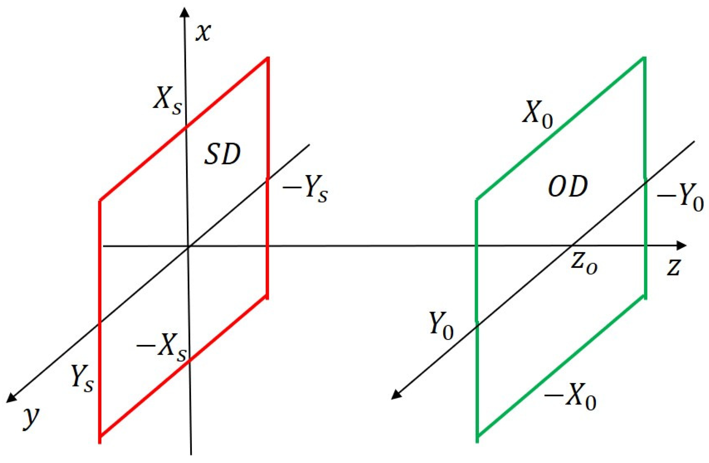
Consider a magnetic current J of bounded finite planar support S D = [ X s , X s ] × [ Y s , Y s ] ( S D stands for source domain) located at z = 0 whose radiated field is observed over another planar domain O D = [ X 0 , X 0 ] × [ Y 0 , Y 0 ] (i.e., the observation domain) located in near-field at z = z o . The source is assumed to be directed in the x y plane whereas only the tangential components of the radiated field are collected. Under this framework, the problem can be split into two scalar problems that can be addressed in the same way. Therefore, here we only consider the current directed along the x-axis, i.e., J = J ( x , y ) x ^ , and collect the corresponding tangential y-component of the radiated field (see Figure 1 for a pictorial view of the configuration).
If we omit an unessential scalar factor, the radiation problem is described in the frequency domain by the following radiation operator
A : J ( r ) X = L 2 ( S D ) ( A J ) ( r o ) = E ( r o ) = S D K ( r o , r ) e j Φ ( r o , r ) J ( r ) d r Y = L 2 ( O D ) ,
with L 2 ( S D ) and L 2 ( O D ) being the set of square integrable functions supported over the source and the observation domains, respectively, r o O D and r S D are the field and the source points and k the free-space wavenumber. Moreover, Φ ( r o , r ) = k | r o r | and K ( r o , r ) = 1 | r o r | 2 [ j k + 1 | r o r | ] j k | r o r | 2 , where the last approximation is because | r o r | z o λ , λ being the free-space wavelength.
We are concerned with the design of a sampling scheme for the observation variable r o which allows to dicretize the data space in such a way to approximate the singular values of A up to a certain index. As is well-known, the singular system { u n , σ n , v n } n = 0 of A , with σ n being the singular values and u n and v n the singular functions that span the source and the field spaces, solves the following equations
σ n v n = A u n σ n u n = A v n ,
where A is the adjoint of the radiation operator defined as
A : f ( r o ) Y = L 2 ( O D ) ( A f ) ( r ) = g ( r ) = O D K ( r o , r ) e j Φ ( r o , r ) f ( r o ) d r o X = L 2 ( S D ) ,
with f and g being two generic functions belonging to Y and X, respectively. However, for our purposes, it is convenient to address the associated eigenvalue problem
σ n 2 v n = A A v n .
Since its finite dimensional approximation entails to discretize r o only. Therefore, in the following we focus on A A whose explicit expression, apart from an unessential constant, is
( A A v n ) ( r o ) = O D d r o S D d r K ( r o , r ) K * ( r o , r ) v n ( r o ) e j [ Φ ( r o , r ) Φ ( r o , r ) ] .
In order to devise the sampling scheme, the main idea it to recast the kernel function of A A as a Fourier-like transformation. To this end, it is convenient to rewrite the phase term as
Φ ( r o , r ) Φ ( r o , r ) = ν 0 ν 1 p Φ ( p ( ν ) , r ) d p ( ν ) d ν d ν ,
with p denotes the gradient with respect to p , such that p ( ν ) is a curve whose starting and ending points coincide with r o and r o , respectively, that is p ( ν 0 ) = r o and p ( ν 1 ) = r o . Now, the curve p ( ν ) can be properly chosen in order to let the phase term resemble a Fourier kernel. This can be achieved, for example, in the following way. Consider r ˜ o ( x o , y o ) and then perform integration in (6) along the polygonal line with nodes r o , r ˜ o and r o , i.e., integration is performed along the segment joining r o and r ˜ o and followed by the segment joining r ˜ o and r o . Accordingly, we have that
Φ ( r o , r ) Φ ( r o , r ) = w ( r o , r o , r ) · ( r o r o ) ,
where · denotes the scalar product, w ( w x , w y ) and
w x ( x o , r o , r ) = 0 1 Φ ( p x , y o , r ) p x p x = x o + ν ( x o x o ) d ν ,
w y ( r o , y o , r ) = 0 1 Φ ( x o , p y , r ) p y p y = y o + ν ( y o y o ) d ν .
Now, it can be shown that r o , r o the transformation w : r w ( r o , r o , r ) is injective and the corresponding Jacobian matrix full rank (the details concerning this point have been omitted for brevity). This allows us to replace in (5) the integration in r with the integration in w , which yields
( A A v n ) ( r o ) = O D d r o Ω ( r o , r o ) d w H ( r o , r o , w ) v n ( r o ) e j w · ( r o r o ) ,
with
Ω ( r o , r o ) = { ( w x ( x o , r o , r ) , w y ( r o , y o , r ) ) : r S D } ,
being the corresponding integration domain in the w variable and
H ( r o , r o , w ) = ( x , y ) ( w x , w y ) K ( r o , r ( w ) ) K * ( r o , r ( w ) ) ,
is the corresponding amplitude term which includes the Jacobian determinant, i.e., ( x o , y o ) ( w x , w y ) , of the variable transformation from r to w . To proceed further we focus on the kernel function of (10), which is given by
k e r n ( r o , r o ) = Ω ( r o , r o ) d w H ( r o , r o , w ) ) e j w · ( r o r o ) .
In order to slightly simplify the previous expression, we note that, because H ( r o , r o , w ) is a constant sign function, Equation (13) clearly shows that the leading order contribution occurs for r o r o = 0 [28]. This allows us to approximate the amplitude factor by its value assumed for r o = r o , that is
H ( r o , r o , w ) H ( r o , r o , w ) = H ( r o , w ) = ( x , y ) ( w x , w y ) | K ( r o , r ( w ) ) | 2 .
By observing that the Jacobian transformation yields
( x , y ) ( w x , w y ) = k 2 z o 2 | r o r | 4 1 = 1 / | K ( r o , r ( w ) ) | 2 ,
we finally have H ( r o , w ) = 1 and the kernel function is eventually approximated as
k e r n ( r o , r o ) = Ω ( r o , r o ) e j w · ( r o r o ) d w .
It is interesting to highlight that (16) shows the kernel function as a 2D spatially varying band-limited function [29], which allows us to expect a non-uniform sampling. This indeed has been already reported in previous contributions [25,30,31,32,33] for one-dimensional currents.

3. Sampling Scheme

In order to devise the sampling scheme, we look for a sampling expansion approximation of the kernel (16). To this end, we extend the approach in [25]. Here, the matter is much more difficult because, unlike as in [25], both the size and the shape of the band Ω ( r o , r o ) change with the observation variable.
To deal with the change in shape of Ω ( r o , r o ) as r o and r o range within O D , we content to approximate (16) by considering a rectangular domain Ω R ( r o , r o ) = [ w m x Δ w x , w m x + Δ w x ] × [ w m y Δ w y , w m y + Δ w y ] that contains Ω ( r o , r o ) . In order to determine Ω R ( r o , r o ) , we have to compute the extreme points of Ω ( r o , r o ) along w x and w y . This is equivalent in determining w x m a x ( x o , r o ) = max r S D { w x ( x o , r o , r ) } , w x m i n ( x o , r o ) = min r S D { w x ( x o , r o , r ) } , w y m a x ( r o , y o ) = max r S D { w y ( r o , y o , r ) } and w y m i n ( r o , y o ) = min r S D { w y ( r o , y o , r ) } . The latter is a tedious but not a complex task and is pursued in Appendix A under the assumption O D S D . Accordingly, once these extreme points have been determined, the parameters of Ω R ( r o , r o ) follow as
Δ w x ( x o , x o ) = ( w x m a x w x m i n / 2 w m x ( x o , x o ) = ( w x m a x + w x m i n ) / 2 Δ w y ( y o , y o ) = ( w y m a x w y m i n ) / 2 w m y ( y o , y o ) = ( w y m a x + w y m i n ) / 2 .
At this juncture, by extending the integration in (16) over the estimated rectangular domain Ω R ( r o , r o ) , the following closed-form approximation of the kernel function is obtained
k e r n ^ R ( r o , r o ) = 4 e j w m · ( r o r o ) Δ w x Δ w y s i n c [ Δ w x ( x o x o ) ] s i n c [ Δ w y ( y o y o ) ] ,
with w m = ( w m x , w m y ) and s i n c ( x ) = sin ( x ) / x .
The parameters of Ω R ( r o , r o ) reported in (17) are spatially varying with the observation variable. This dependence can be removed by introducing a suitable ‘warping’ transformation [34,35,36]. This task is relatively easy under the assumption O D S D (see Appendix A). Indeed, in this case the warping transformation ‘factorizes’, in the sense that the observation variables x o and y o can be warped independently from each other. In particular, such transformations are (see Appendix A for details)
ξ x : x o ξ x ( x o ) = k 2 [ ( x o + X s ) 2 + z o 2 ( x o X s ) 2 + z o 2 ] ξ y : y o ξ y ( y o ) = k 2 [ ( y o + Y s ) 2 + z o 2 ( y o Y s ) 2 + z o 2 ] ,
and
γ x : x o γ x ( x o ) = k 2 [ ( x o + X s ) 2 + z o 2 + ( x o X s ) 2 + z o 2 ] γ y : y o γ y ( y o ) = k 2 [ ( y o + Y s ) 2 + z o 2 + ( y o Y s ) 2 + z o 2 ] .
Accordingly, Equation (18) rewrites as (see Appendix A for further details)
k e r n ^ R ( r o , r o ) = 4 e j ( γ x ( x o ) γ x ( x o ) ) e j ( γ y ( y o ) γ y ( y o ) ) Δ w x Δ w y s i n c [ ξ x ( x o ) ξ x ( x o ) ] s i n c [ ξ y ( y o ) ξ y ( y o ) ] .
Basically, Equation (19) and Equation (20) transform the rectangular region in ( x o , y o ) , i.e., the actual observation domain O D = [ X 0 , X 0 ] × [ Y 0 , Y 0 ] , into the rectangular domain [ Δ ξ x , Δ ξ x ] × [ Δ ξ y , Δ ξ y ] of the ( ξ x , ξ y ) plane, with
Δ ξ x = ( ξ x m a x ξ x m i n ) / 2 = k 2 [ z o 2 + ( X 0 + X s ) 2 z o 2 + ( X 0 X s ) 2 ] Δ ξ y = ( ξ y m a x ξ y m i n ) / 2 = k 2 [ z o 2 + ( Y 0 + Y s ) 2 z o 2 + ( Y 0 Y s ) 2 ] ,
with ξ x m a x and ξ x m i n being the maximum and the minimum of the function ξ over the allowed values of x o , and ξ y m a x and ξ y m i n are the analogous for the ξ y function.
Now, we can finally rewrite the eigenvalue problem in (10) in the warped domain ( ξ x , ξ y ) by changing the integration variable from ( x o , y o ) to ( ξ x , ξ y ) . Accordingly, the singular functions spanning the field space can be expressed as
σ n 2 v ¯ n ( ξ x , ξ y ) = ( A A v ¯ n ) ( ξ x , ξ y ) =
Δ ξ x Δ ξ x d ξ x Δ ξ y Δ ξ y d ξ y 4 Δ w x Δ w y | ( x o , y o ) ( ξ x , ξ y ) | k e r n ¯ ( ξ x , ξ y , ξ x , ξ y ) v ¯ n ( ξ x , ξ y ) ,
where ξ x = ξ x ( x o ) , ξ y = ξ y ( y o ) , v ¯ n ( ξ x , ξ y ) = v n ( ξ x , ξ y ) e j γ x ( ξ x ) e j γ y ( ξ y ) , | ( x o , y o ) ( ξ x , ξ y ) | is the Jacobian determinant related to the transformation variables from ( x o , y o ) to ( ξ x , ξ y ) and
k e r n ¯ = s i n c [ ξ x ( x o ) ξ x ( x o ) ] s i n c [ ξ y ( y o ) ξ y ( y o ) ] .
By employing similar reasoning used for the amplitude term in (16) we made Section 2, we approximate Δ w x ( x o , x o ) = Δ w x ( x o , x o ) = Δ w x ( x o ) and Δ w y ( y o , y o ) = Δ w y ( y o , y o ) = Δ w y ( y o ) . This yields
4 Δ w x Δ w y | ( x o , y o ) ( ξ x , ξ y ) | = 1 ,
and (23) becomes
σ n 2 v ¯ n ( ξ x , ξ y ) = ( A A v ¯ n ) ( ξ x , ξ y ) = Δ ξ x Δ ξ x d ξ x Δ ξ y Δ ξ y d ξ y k e r n ¯ ( ξ x , ξ y , ξ x , ξ y ) v ¯ n ( ξ x , ξ y ) .
The advantage provided by reformulating the eigenvalue problem as in (26) is evident since we are now allowed to use the standard sampling theorem (with respect to the introduced warped variables) [26] to build the discrete version of A A for eingenspectrum computation [37]. More in detail, Equation (26) says that v ¯ n are band-limited functions (because k e r n ¯ is a band-limited function) and hence can be expanded as
v ¯ n ( ξ x , ξ y ) = m , l v ¯ n ( ξ x m , ξ v l ) s i n c [ ξ x ξ x m ] s i n c [ ξ y ξ y l ] ,
with ξ x m = m π and ξ y l = l π being the sampling points and m and l integer indexes. Of course, since the singular functions v ¯ n span the field space the same expansion holds true for the field. Hence, Equation (27) is the sampling expansion we were looking for. In particular, in order to pass from the sampling points in ( ξ x , ξ y ) to the ones in ( x o , y o ) (the actual observation variables), Equation (19) must be used. For example, the sampling position along x o , i.e., x o m , are obtained by solving for x o m the following equation
k 2 [ z o 2 + ( x o m + X s ) 2 z o 2 + ( x o m X s ) 2 ] = ξ x m = m π ,
or equivalently
k 2 x o m 2 ξ x m 2 k 2 z o 2 k 2 ξ x m 2 = 1 .
A similar equation of course holds true for the sampling points y o m along the variable y o .
In order to appreciate the goodness of the proposed sampling scheme, we need to obtain the discrete version of the eigenvalue problem (10). This is achieved by inserting (27) into (26), that yields
σ n 2 v ̲ n = B v ̲ n ,
where v ̲ n is the vectorized form of the matrix consisting of the samples of v ¯ n and the entries of the matrix, B α , β , are given by
B α ( m , l ) , β ( s , t ) = Δ ξ x Δ ξ x d ξ x Δ ξ y Δ ξ y d ξ y k e r n ¯ ( m π , l π , ξ x , ξ y ) s i n c ( ξ x s π ) s i n c ( ξ y t π ) .
Note that the integer indexes m, l and s and t range over the two-dimensional sampling lattice involved by (27) and the matrix entry indexes α and β vary according to the way the vectorization of v ̲ n is achieved.
It is worth remarking that B describes an infinite discrete problem. However, since (27) must be used to represent the field over the measurement aperture, we are allowed to retain only the samples falling within [ Δ ξ x , Δ ξ x ] × [ Δ ξ y , Δ ξ y ] , which corresponds to the observation domain O D . Accordingly, in the sequel, we will consider a truncated version of B , i.e., B N of size N × N , which takes into account only the samples falling within the observation domain. More in detail, N = N x N x and N x = [ 2 Δ ξ x / π ] , N y = [ 2 Δ ξ y / π ] , [ · ] being the operator that takes the integer part. Indeed, for classical band-limited kernels, N represents the so-called Shannon number ( S N ) which is known to give a good estimation of the number of degrees of freedom [23,37]. In particular, in these cases, the singular values exhibit a step-like behavior and the S N basically returns the number of singular values preceding the abrupt decay. However, it also known that to properly capture that part of the singular value behavior, and also to go a bit beyond the ’knee’, a slightly greater number of samples are required [37]. Therefore, in the following numerical analysis, an oversampling factor of 1.3 is considered, that is to say, that the sampling step (in ξ x and ξ y ) is fixed at π / 1.3 .

4. Numerical Analysis

In this section, we check the previous theoretical findings by some numerical examples.
We start by first verifying if the proposed sampling scheme works in approximating the singular values of the radiation operator. Note that the singular values of A are the square root of the eigenvalues of A A . Therefore, in the sequel, we will speak about the singular values or the eigenvalues without distinction.
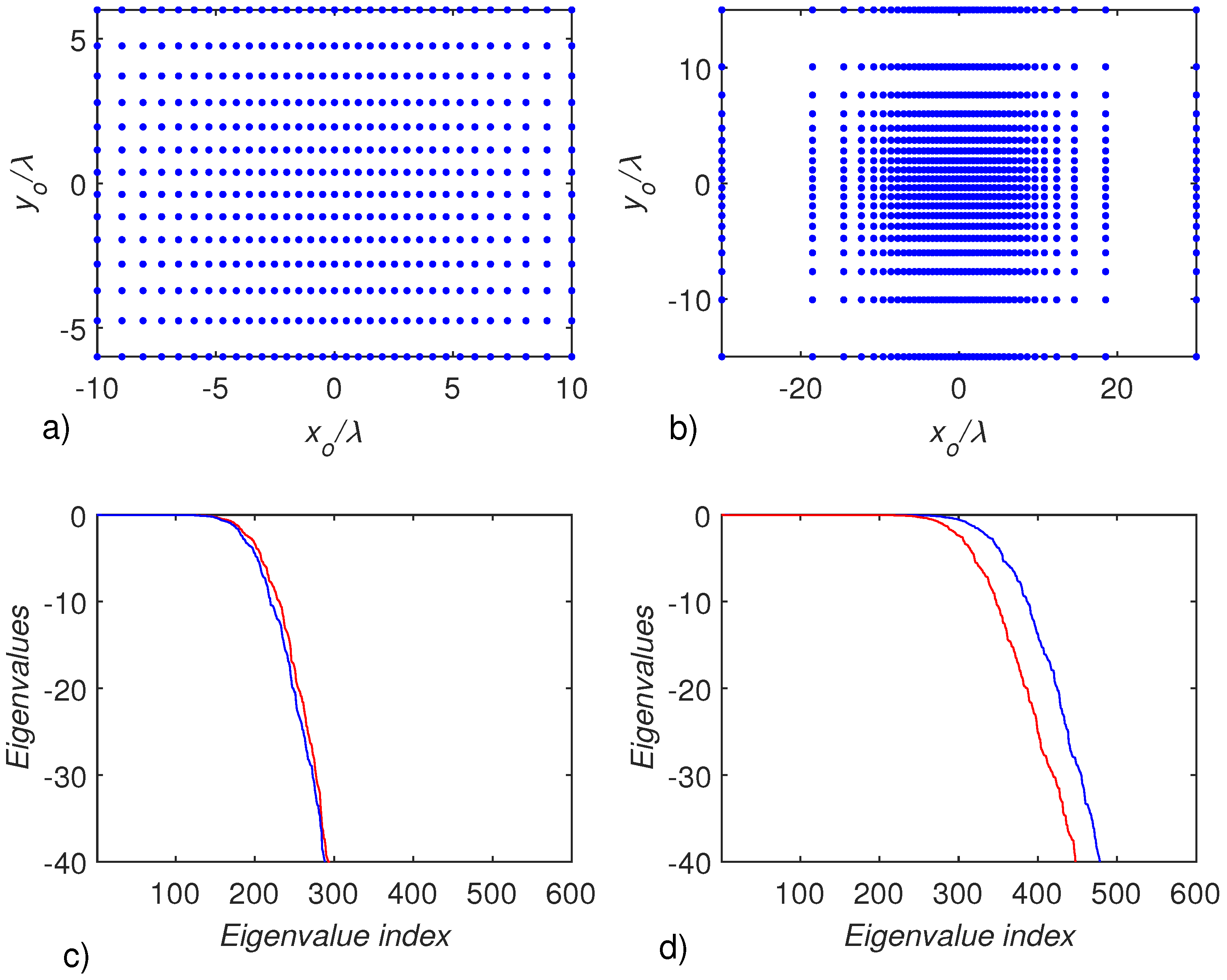
We consider a source domain S D = [ 8 λ , 8 λ ] × [ 4 λ , 4 λ ] (with X s = 8 λ and Y s = 4 λ ) and assume to collect the data over two measurement domains both located at z o = 7 λ : the first one is O D 1 = [ 10 λ , 10 λ ] × [ 6 λ , 6 λ ] (with X 0 = 10 λ and Y 0 = 6 λ ); the second one is O D 2 = [ 30 λ , 30 λ ] × [ 15 λ , 15 λ ] (with X 0 = 10 λ and Y 0 = 6 λ ). The corresponding results are reported in Figure 2. In particular, in panels (a) and (b) the sampling point distributions returned by the proposed non-uniform sampling scheme are sketched for the two considered observation domains. Panels (c) and (d) instead report the comparison between the eigenvalues of B N and A A . According to the theoretical derivation, we have a strict constraint on the size of the measurement aperture which should not exceed the one of the source. Nonetheless, in both the cases considered in Figure 2, the observation domain violates such a constraint, especially for the example reported in panels (b) and (d). By looking at such a figure the following conclusions can be drawn. First, the proposed sampling scheme is able to very well approximate the eigenvalues even when the observation domain O D slightly exceeds the source domain S D (see panel (c) which refers to O D 1 ). Instead, in panel (d), where O D 2 is much larger than S D , it is evident that the number of degrees of freedom is underestimated since the ‘knee’ of the eigenvalues starts before the actual one. This means that the sampling points are not enough (and not properly located). However, the initial part of the eigenvalue behavior is very well-approximated. Hence, we conclude that in this case, the proposed non-uniform sampling strategy is able to approximate only a subset of all possible radiated fields, i.e., the ones spanned by the singular functions corresponding to the singular values that are well-estimated. As a consequence, it is expected that the non-uniform sampling can allow for a good radiated field approximation if the field significantly projects on those singular functions, even when the constraint on the size of O D is not strictly verified.
The second important point that must be highlighted is that the number of samples required by the proposed sampling scheme is actually much lower than the ones arising from a λ / 2 sampling. Indeed, for the two cases, our method requires N = 462 and N = 840 , respectively for O D 1 and O D 2 , whereas the λ / 2 sampling requires 1025 and 7381 samples.
In order to appreciate the capability of the proposed sampling method of approximating the radiated field, we use the following relative error metric ( R E ) computed over the measurement aperture, that is
R E d B ( X 0 , Y 0 ) = 20 log 10 | | E E λ / 2 | | | | E λ / 2 | | ,
where E is the near-field obtained by collecting the data according to the proposed non-uniform sampling scheme and then interpolated over a λ / 2 grid, E λ / 2 is the near-field data directly collected over the uniform λ / 2 grid and · is the Euclidean norm. In order to highlight the role of the type of source, three different source distributions defined over ( x , y ) S D = [ 8 λ , 8 λ ] × [ 4 λ , 4 λ ] are considered, that is
  • J 1 ( x , y ) = cos 2 ( π x 2 X s ) e j k sin ( π / 20 ) cos ( π / 4 ) x cos 2 ( π y 2 Y s ) e j k sin ( π / 20 ) sin ( π / 4 ) y ;
  • J 2 ( x , y ) = 1 ;
  • J 3 ( x , y ) = 4 cos [ k sin ( π / 4 ) cos ( π / 4 ) x ] cos [ k sin ( π / 4 ) sin ( π / 4 ) y ] .
More in detail, the first source gives rise to very low side-lobes and hence it has been considered to see if, and to what extent, they can be estimated by using the proposed sampling scheme. The second source is constant and presents an abrupt decay at the edges of the source domain; its radiation pattern is a sinc-like function. Finally, the third current leads to a steered multi-beam radiation pattern. Basically, these examples present a growing level of difficulty, since moving from J 1 to J 3 the currents project over a large number of singular functions.
In Table 1, the relative error R E is given in dB for the different sources under consideration and the two measurement apertures addressed in Figure 2. As can be seen, for O D 1 = [ 10 λ , 10 λ ] × [ 6 λ , 6 λ ] , the error is relatively low for all the sources. This means that the proposed sampling scheme returns a good approximation for the near-field although the number of samples has been greatly reduced as compared to the λ / 2 sampling scheme. This was indeed expected since the proposed sampling scheme works well if the observation domain O D is similar in size to the source domain S D . When the measurement aperture is increased (see the third column of Table 1) the error decreases for J 1 ( x , y ) and J 2 ( x , y ) and increases for J 3 ( x , y ) . This is because the field radiated by J 1 and J 2 significantly projects on the singular functions corresponding to the singular values that are well-approximated (see panel (d) of Figure 2). Accordingly, the metric error benefits from the higher number of sampling points (that are required since O D 2 is larger than O D 1 ) that can be used to perform the interpolation. On the contrary, for J 3 , the error increases because the radiated field also projects on the singular functions of A which are not well-approximated by our discretization scheme. In other words, the field radiated by J 3 is also relevant for the points of O D 2 which exceed the limit of O D 1 and hence of S D .
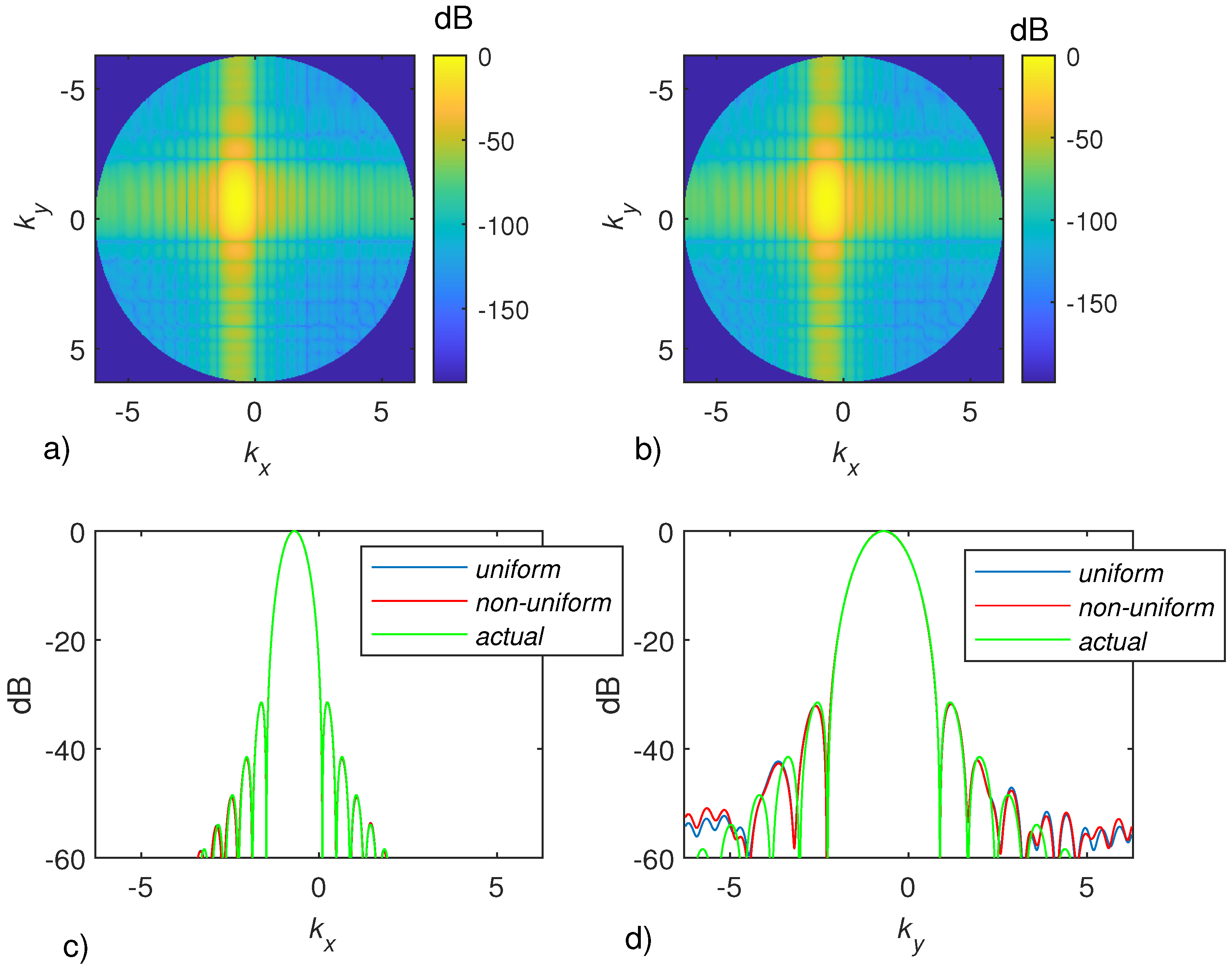
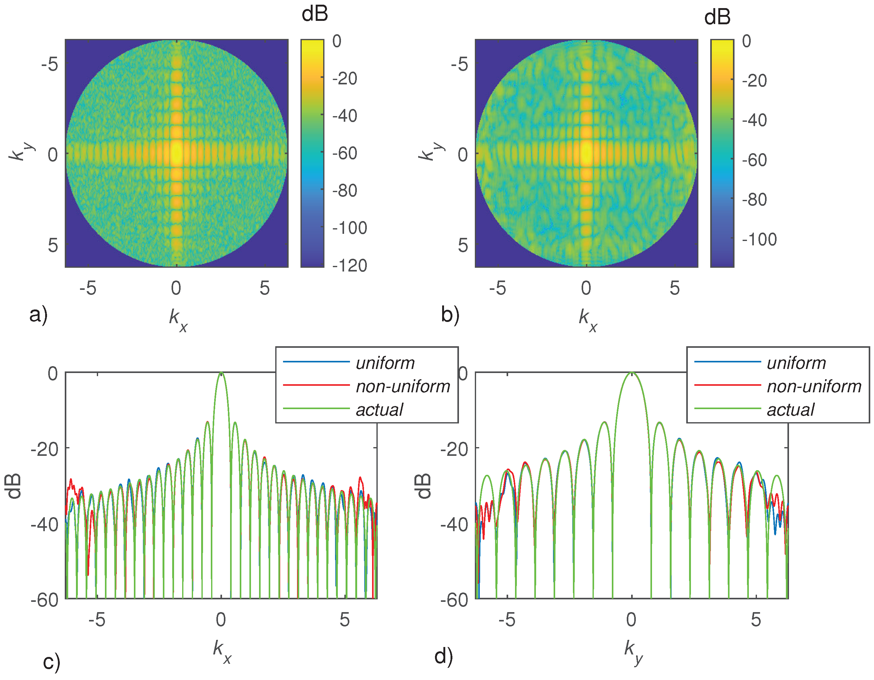
We now pass to analyzing the radiation patterns which are obtained by Fourier transforming (by means of a FFT procedure) the near-field data. The radiation patterns are reported as a function of the spectral variables k x = k sin θ cos ϕ and k y = k sin θ sin ϕ , with θ and ϕ being the usual polar angles, and shown only for the so-called ’visible’ domain, that is for k x 2 + k y 2 = k 2 . More in detail, after collecting the field data according to the proposed non-uniform sampling scheme, the field is interpolated over a uniform λ / 2 grid and finally, Fourier transformed.
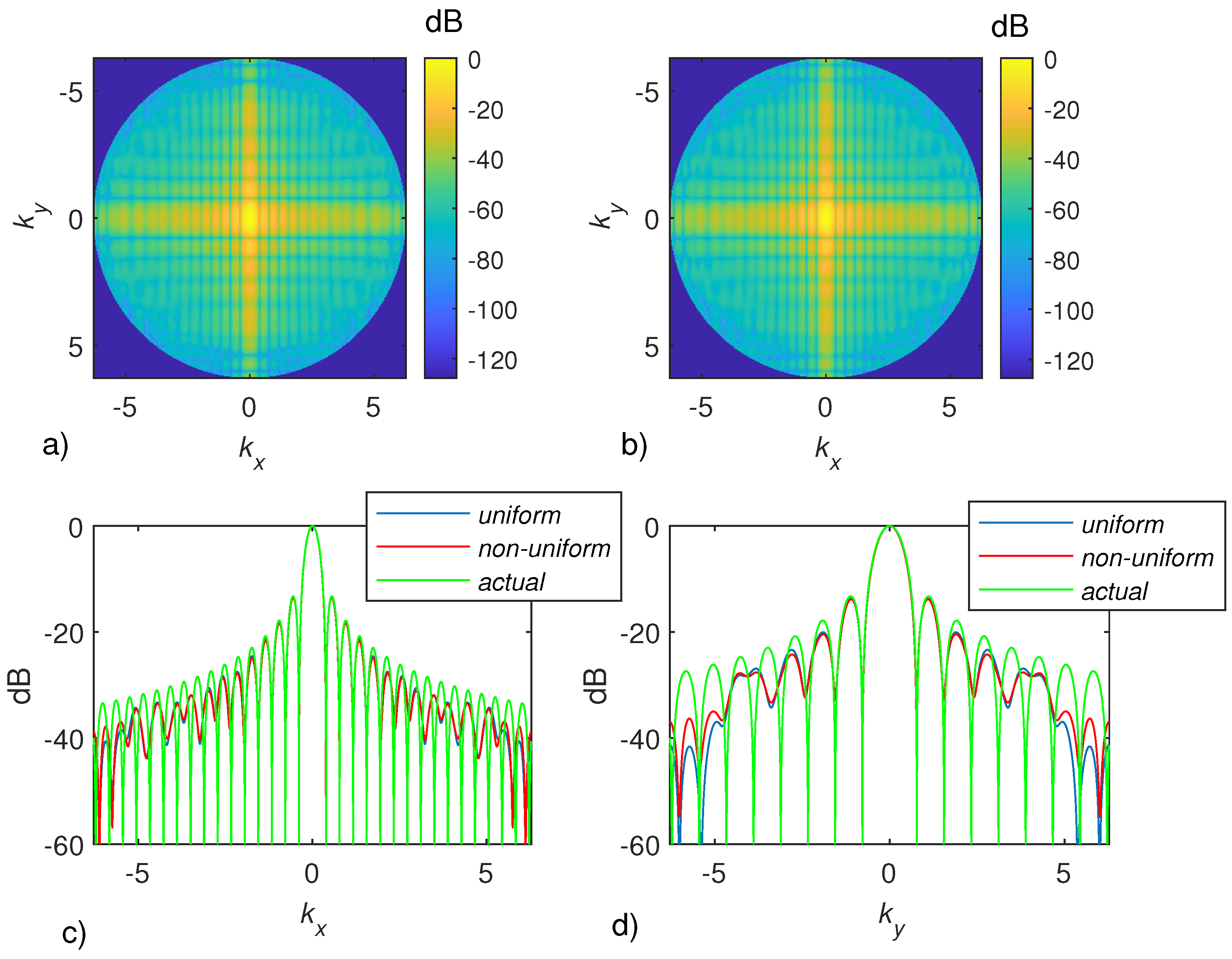
The radiation pattern corresponding to J 1 is reported in Figure 3 and Figure 4 for the measurement aperture O D 1 and O D 2 , respectively. For example, by comparing panels (a) and (b) of Figure 3 the radiation patterns computed by using the proposed method and the usual uniform sampling look very similar. This can be even better appreciated by looking at the cut-views shown in panels (c) and (d), where the blue lines refer to the radiation pattern computed by using the uniform λ / 2 sampling and the red ones to the radiation pattern obtained by the proposed method. In particular, herein, the actual radiation pattern (in green lines) is also reported for comparison purposes. Since for this case, the non-uniform sampling succeeds in approximating well the near-field (see Table 1) this very good match between the radiation patterns computed by using the two sampling schemes under comparison was indeed expected. In particular, they also exhibit a similar truncation error in the very low side-lobe region along k y (see panel (d)). This, of course, is because the observation domain is shorter along y axis. However, this error is dramatically reduced in 
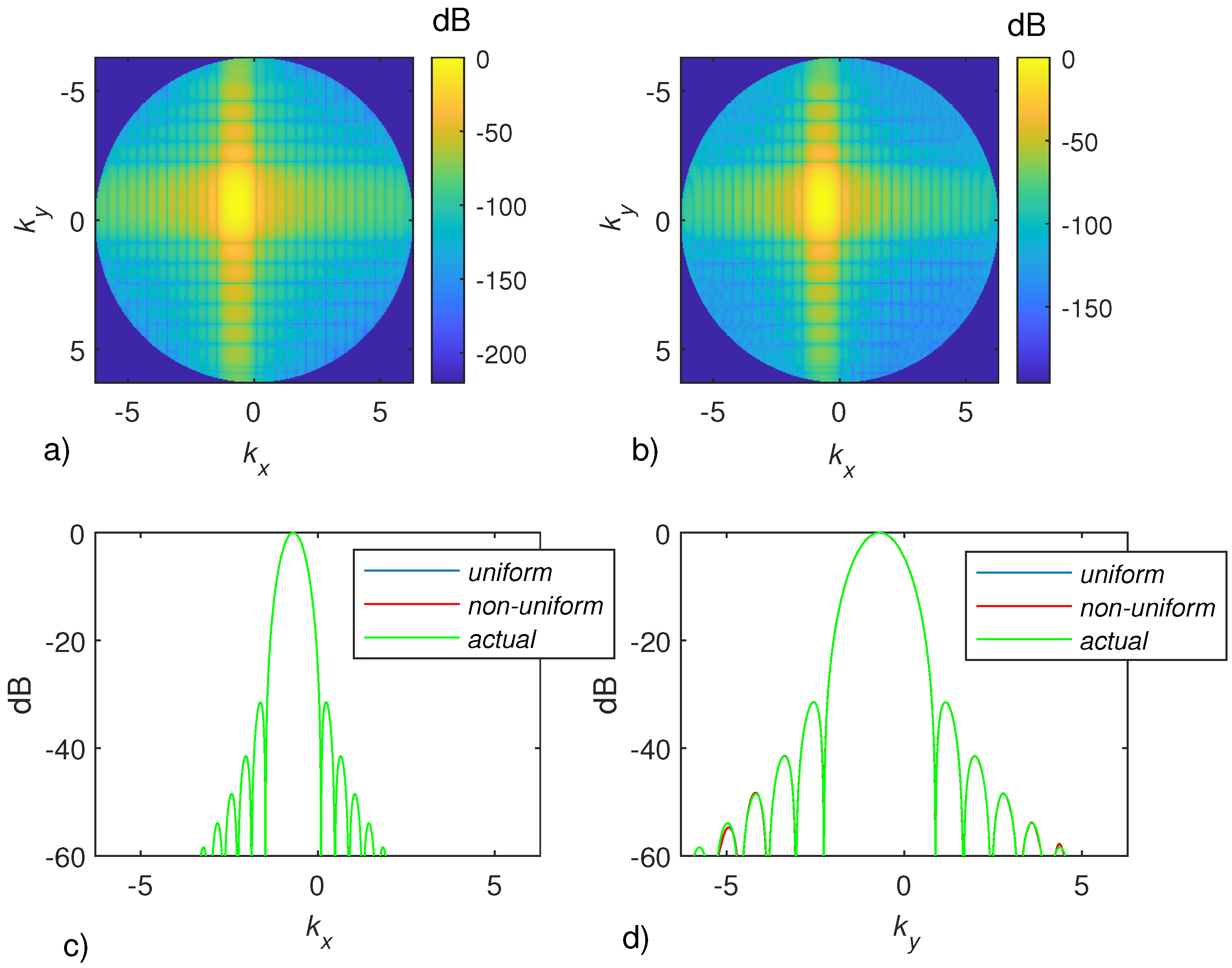
Figure 4 where the larger measurement aperture O D 2 was considered. In fact, since in this case, the aperture has been enlarged and the radiated field still projects well on the singular functions that have been well-approximated through the non-uniform sampling, the three lines overlap very well and appear indistinguishable.
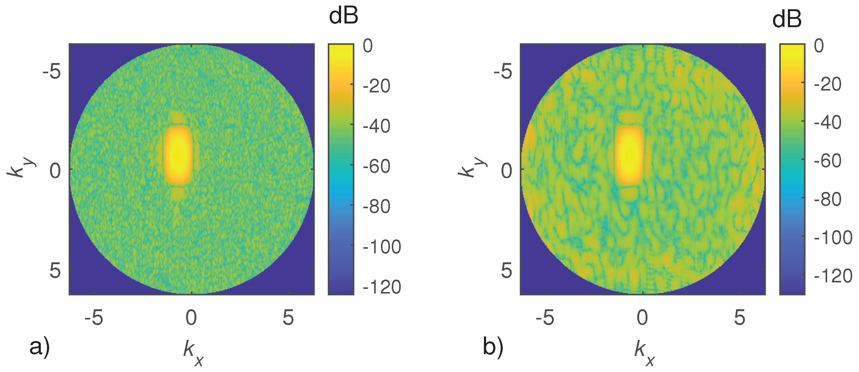
In Figure 5, we consider the same case as in Figure 4 but a complex white Gaussian noise is added to the field data. In particular, a signal to noise ratio (SNR), defined as
S N R = | | E | | | | N | | ,
with E the field data and N the noise, of 20 dB is considered. As can be seen, the two sampling schemes still return similar results (in particular look at panels (c) and (d)). Indeed, both succeed in approximating the first side-lobe of the actual radiation pattern whereas the very low side-lobe region is definitely affected by the noise. However, what matters here is that, though much fewer sampling points have been used by our method, the two sampling schemes show a similar effect of the noise.
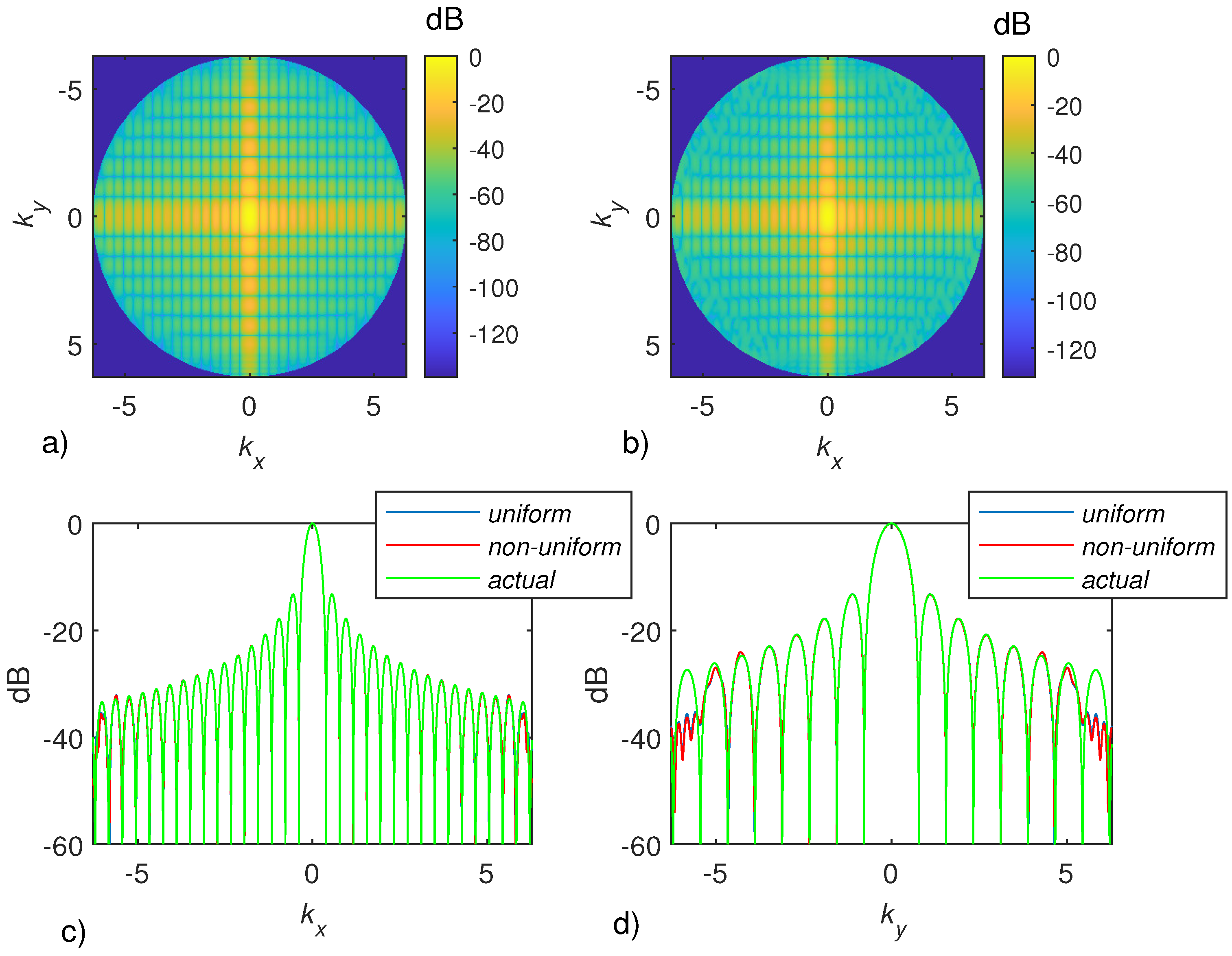
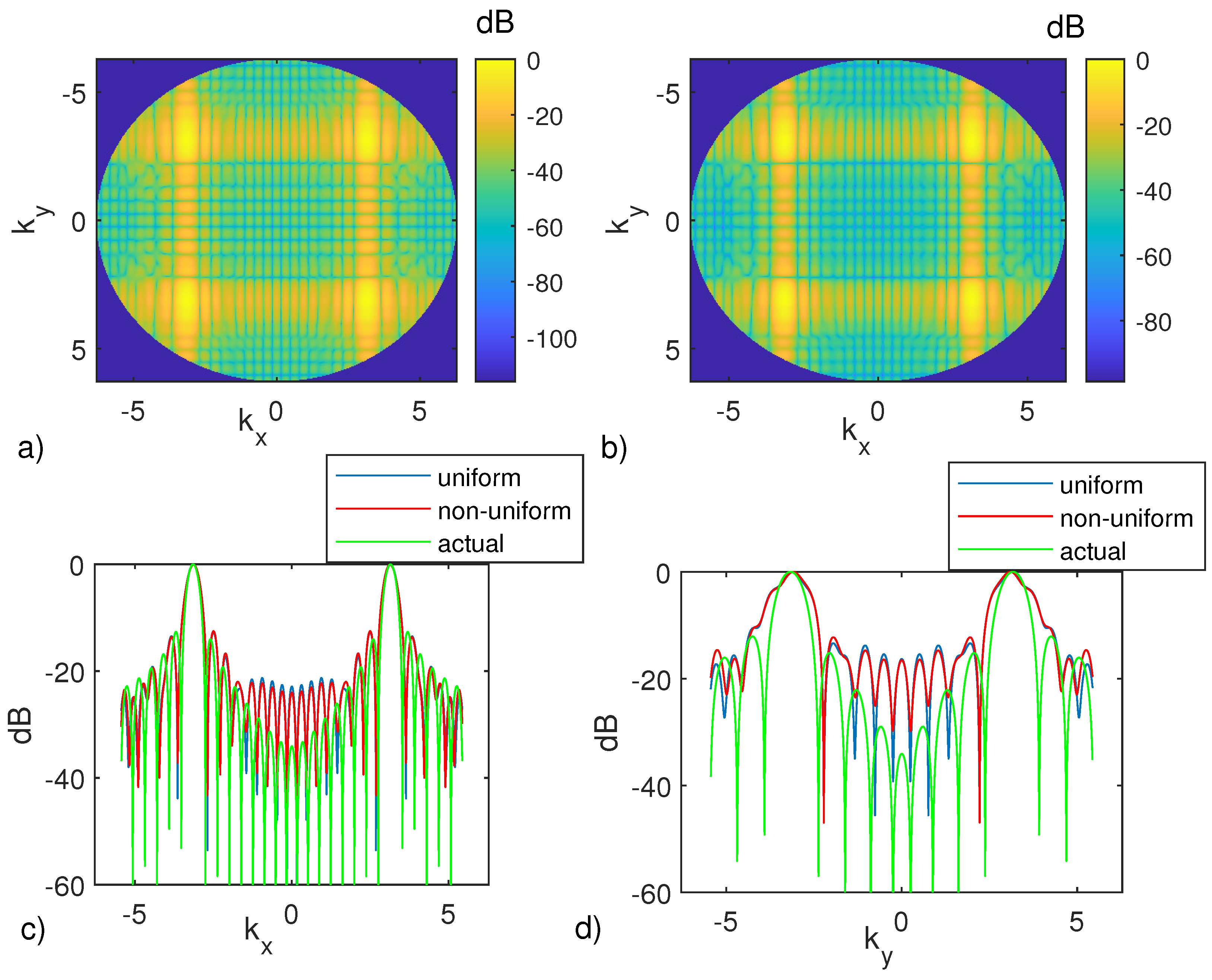
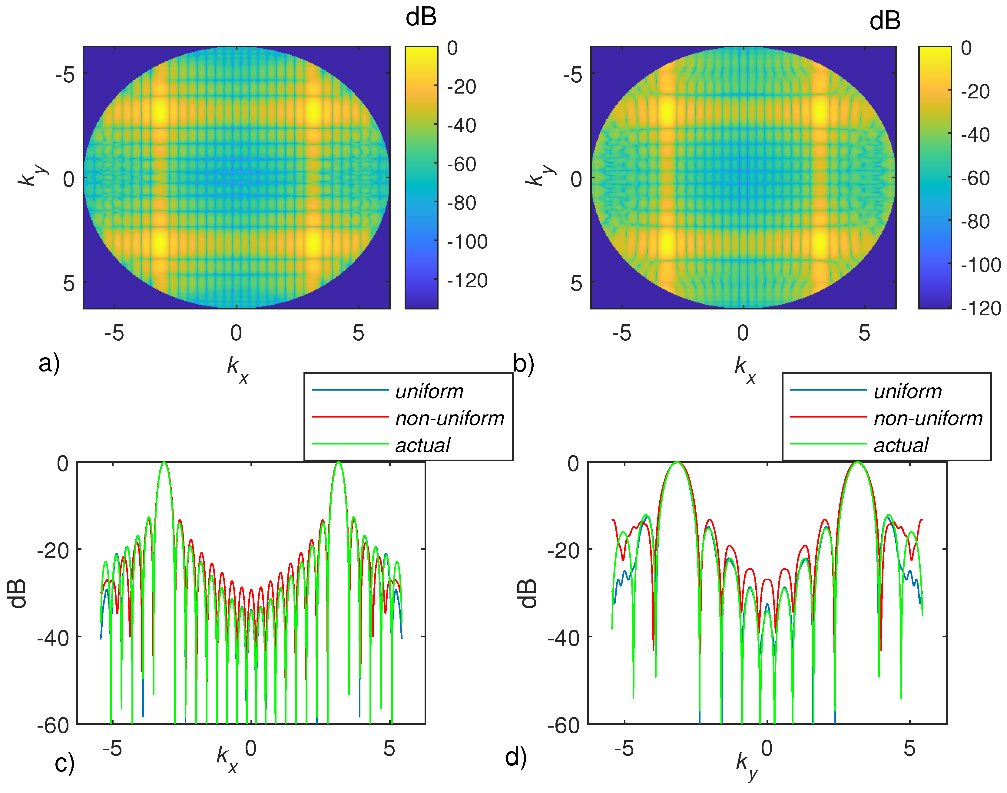
The results concerning J 2 are reported in Figure 6, Figure 7 and Figure 8. In particular, Figure 6 refers to O D 1 , Figure 7 to O D 2 and Figure 8 to O D 2 with noisy data and S N R = 20 dB. By looking at Figure 6 it can be appreciated that the radiation pattern computed by the two sampling schemes are still very similar and both exhibit a relevant truncation error (see panels (c) and (d)) since the returned radiation patterns (red and blue lines) are considerably different from the actual one (green lines). This error, however, is reduced to a large extent by increasing the measurement aperture as shown in Figure 7 where the three lines are indistinguishable. Moreover, the estimated radiation pattern through the two sampling schemes shows similar stability against the noise as illustrated in Figure 8.
Finally, Figure 9 and Figure 10 show the results concerning J 3 . According to what was reported at the beginning of this section, since for the case of O D 1 the proposed sampling strategy allows to obtain a good estimation of the near-field, the radiation patterns obtained by the non-uniform and the uniform sampling schemes are very similar for the case of O D 1 addressed in Figure 9. However, because of the size of O D 1 , there is a relevant truncation error, as highlighted in panels (c) and (d) of such a figure. The measurement aperture is enlarged at O D 2 in Figure 10. Now, though the truncation error is significantly reduced for both the sampling schemes, the actual pattern (green lines) is much better approximated by the one returned by the uniform sampling (blue lines) (see panels (c) and (d) of Figure 10). This is because, differently from J 1 and J 2 , J 3 presents relevant components over the singular functions that are not well-approximated by the non-uniform sampling scheme. This clearly highlights the role of the type of source.
Summarizing, regardless of the type of source, the proposed sampling strategy returns a good estimation for the near-field when the observation domain, O D , is equal or ‘slightly’ larger than the source domain, S D . When the measurement aperture is much larger than S D , the representation error depends on the type of sources and is relevant if the source significantly projects on the singular functions of A that are not well-approximated by the proposed discretization strategy. In the latter case, the estimated radiation pattern can suffer from a large deviation from the actual one. Therefore, it can be concluded that the method is better suited to broadside antennas and further theoretical work is required to generalize the sampling scheme to the case of beam-steered antennas.

5. Conclusions

In this paper, the problem of sampling the field radiated by a planar source and observed over a finite planar aperture located in the near-field has been addressed. The problem has been cast as the determination of the measurement spatial positions for which the singular values of the radiation operator are well-approximated. Thanks to suitable variable transformations, which ‘warp’ the spatial observation variables, the kernel function of A A has been approximated as a band-limited function and hence the standard sampling theorem used to discretize the problem. Basically, the new content conveyed by this paper consists in the introduction of a sampling scheme which allows us to reduce the number of measurements as compared to the most used sampling scheme in the industry for antenna characterization, to avoid to use of numerical iterative procedures for selecting the measurement positions, to extend our previous results which were concerned for the simpler case of strip currents.
The developed theory rigorously works for measurement apertures that are not too large as compared to the source’s size. Therefore, it has been concluded that the proposed method is better suited to broadside antennas. In this regard, it must be emphasized that the mentioned limitations arise because in the derivation we assumed S D O D . This greatly simplified the problem because it allowed us to find factorized warping transformation and the related sampling scheme. Accordingly, this contribution can be seen as a preliminary contribution that must be generalized in order to deal with larger measurement apertures and general source types. In view of the great reduction in the number of data points, we are stimulated in addressing this question in future developments.
Finally, it worth remarking that besides the radiation pattern estimation, determining how to sample the radiated field is inherently connected to the inverse source problem [38] and also to the computation of the information content that can be ’communicated’ from a source to an observation domain. In fact, it is well-known that the information content (quantified by the Shannon or the Kolmogorov metrics) are explicitly dependent on the singular value behavior of the radiation operator [39].

Author Contributions

Conceptualization, M.A.M., R.P. and R.S.; methodology, M.A.M. and R.S.; software, M.A.M.; writing—original draft preparation, M.A.M.; writing—review and editing, M.A.M., R.P. and R.S.; supervision, R.S.; funding acquisition, R.P. All authors have read and agreed to the published version of the manuscript.

Funding

This research was funded by the Italian Ministry of University and Research through the PON initiative under the project Leonardo 4.0.

Acknowledgments

The authors kindly thank Giuseppina Nuzzo for proofreading the manuscript.

Conflicts of Interest

The authors declare no conflict of interest.

Appendix A

In order to evaluate w m , Δ w x and Δ w y which are relevant for estimating Ω R ( r o , r o ) described in Section 3, we have to compute w x m a x ( x o , r o ) = max r S D { w x ( x o , r o , r ) } , w x m i n ( x o , r o ) = min r S D { w x ( x o , r o , r ) } , w y m a x ( r o , y o ) = max r S D { w y ( r o , y o , r ) } and w y m i n ( r o , y o ) = min r S D { w y ( r o , y o , r ) } . Since the Jacobian of the transformation w : r w ( r o , r o , r ) is full rank, both w x and w y cannot have stationary points inside S D . Therefore, their maxima and minima must be looked for over the boundary of the observation domain. By assuming S D O D and after simple but tedious calculations, it results that
w x m a x ( x o , r o ) = w x ( x o , r o , X s , y = y o ) w x m i n ( x o , r o ) = w x ( x o , r o , X s , y = y o ) w y m a x ( r o , y o ) = w y ( r o , y o , x = x o , Y s ) w y m i n ( r o , y o ) = w y ( r o , y o , x = x o , Y s ) ,
from which it readily follows that
w x m a x ( x o , x o ) = 1 x o x o x o x o k p x + X s ( p x + X s ) 2 + z o 2 d p x w x m i n ( x o , x o ) = 1 x o x o x o x o k p x X s ( p x X s ) 2 + z o 2 d p x w y m a x ( y o , y o ) = 1 y o y o y o y o k p y + Y s ( p y + Y s ) 2 + z o 2 d p y w y m i n ( y o , y o ) = 1 y o y o y o y o k p y Y s ( p y Y s ) 2 + z o 2 d p y .
In particular, Equation (A2) allows to highlight that w x and w y range within intervals that depend only on x o , x o and y o , y o , respectively. This is a very important aspect since it leads to the ’factorized’ sampling expansion presented in Section 3. More in detail, by using (A2) in (17), we obtain
Δ w x ( x o , x o ) = k 2 ( x o x o ) x o x o [ p x + X s ( p x + X s ) 2 + z o 2 p x X s ( p x X s ) 2 + z o 2 ] d p x w m x ( x o , x o ) = k 2 ( x o x o ) x o x o [ p x + X s ( p x + X s ) 2 + z o 2 + p x X s ( p x X s ) 2 + z o 2 ] d p x Δ w y ( y o , y o ) = k 2 ( y o y o ) y o y o [ p y + Y s ( p y + Y s ) 2 + z o 2 p y Y s ( p y Y s ) 2 + z o 2 ] d p y w m y ( y o , y o ) = k 2 ( y o y o ) y o y o [ p y + Y s ( p y + Y s ) 2 + z o 2 + p y Y s ( p y Y s ) 2 + z o 2 ] d p y .
In particular, by solving the integrals
Δ w x ( x o , x o ) = k ( x o + X s ) 2 + z o 2 ( x o + X s ) 2 + z o 2 ( x o X s ) 2 + z o 2 ( x o X s ) 2 + z o 2 2 ( x o x o ) w m x ( x o , x o ) = k ( x o + X s ) 2 + z o 2 ( x o + X s ) 2 + z o 2 ( x o X s ) 2 + z o 2 + ( x o X s ) 2 + z o 2 2 ( x o x o ) Δ w y ( y o , y o ) = k ( y o + y s ) 2 + z o 2 ( y o + y s ) 2 + z o 2 ( y o y s ) 2 + z o 2 ( y o y s ) 2 + z o 2 2 ( y o y o ) w m y ( y o , y o ) = k ( y o + y s ) 2 + z o 2 ( y o + y s ) 2 + z o 2 ( y o y s ) 2 + z o 2 + ( y o y s ) 2 + z o 2 2 ( y o y o ) .
Finally, by using the warping transformations presented in (19) and (20), it readily follows that w m x ( x o x o ) = γ x ( x o ) γ x ( x o ) , w m y ( y o y o ) = γ y ( y o ) γ y ( y o ) , Δ w x ( x o x o ) = ξ x ( x o ) ξ x ( x o ) and Δ w y ( y o y o ) = ξ y ( y o ) ξ y ( y o ) , and hence from (18) the kernel expression in (21) is obtained.

References

  1. Gillespie, E.S. Preface. IEEE Trans. Antennas Propag. 1988, 36, 725–726. [Google Scholar]
  2. Yaghjian, A.D. An overview of near-field antenna measurements. IEEE Trans. Antennas Propag. 1986, 34, 30–45. [Google Scholar] [CrossRef] [Green Version]
  3. Francis, M.H.; Wittmann, R.W. Near-field scanning measurements: Theory and practice. In Modern Antenna Handbook; Balanis, C.A., Ed.; John Wiley & Sons: Hoboken, NJ, USA, 2008; pp. 929–976. [Google Scholar]
  4. Capozzoli, A.; Celentano, L.; Curcio, C.; Liseno, A.; Savarese, S. Twice optimised near-field scanning system for antenna characterisation. IET Microw. Antennas Propag. 2020, 14, 163–173. [Google Scholar] [CrossRef]
  5. Hansen, T.B.; Yaghjian, A.D. Plane-Wave Theory of Time-Domain Fields: Near-Field Scanning Applications; Wiley-IEEE Press: Hoboken, NJ, USA, 1999. [Google Scholar]
  6. Leach, W.; Paris, D. Probe compensated near-field measurements on a cylinder. IEEE Trans. Antennas Propag. 1973, AP-21, 435–445. [Google Scholar] [CrossRef]
  7. Breinbjerg, O. Spherical Near-Field Antenna Measurements—The Most Accurate Antenna Measurement Technique. In Proceedings of the 2016 IEEE International Symposium on Antennas and Propagation (APSURSI), Fajardo, Puerto Rico, 26 June–1 July 2016; pp. 1019–1020. [Google Scholar]
  8. Varela, F.R.; Iragüen, B.G.; Sierra-Castañer, M. Near-Field to Far-Field Transformation on Arbitrary Surfaces via Multi-Level Spherical Wave Expansion. IEEE Trans. Antennas Propagat. 2020, 68, 500–508. [Google Scholar] [CrossRef]
  9. Schmidt, C.H.; Eibert, T.F. Multilevel Plane Wave Based Near-Field Far-Field Transformation for Electrically Large Antennas in Free-Space or Above Material Halfspace. IEEE Trans. Antennas Propagat. 2009, 57, 1382–1390. [Google Scholar] [CrossRef]
  10. Bucci, O.M.; Gennarelli, C.; Savarese, C. Representation of Electromagnetic Fields over Arbitrary Surfaces by a Finite and Nonredundant Number of Samples. IEEE Trans. Antennas Propagat. 1998, 46, 351–359. [Google Scholar] [CrossRef]
  11. Maisto, M.A.; Solimene, R.; Pierri, R. Optimal choice of measurement points in near field: Numerical results. In Proceedings of the 2018 IEEE International Symposium on Antennas and Propagation USNC/URSI National Radio Science Meeting, Boston, MA, USA, 8–13 July 2018; pp. 2561–2562. [Google Scholar]
  12. Maisto, M.A.; Solimene, R.; Pierri, R. Efficient Sampling of the Near Field Radiated by a Planar Source: Numerical Results. In Proceedings of the 2019 PhotonIcs & Electromagnetics Research Symposium-Spring (PIERS-Spring), Rome, Italy, 17–20 June 2019; pp. 915–918. [Google Scholar]
  13. D’Agostino, F.; Ferrara, F.; Gennarelli, C.; Guerriero, R.; Migliozzi, M. Fast and accurate far-field prediction by using a reduced number of bipolar measurements. IEEE Antennas Wirel. Propag. Lett. 2017, 16, 2939–2942. [Google Scholar] [CrossRef]
  14. Migliore, M.D. Near Field Antenna Measurement Sampling Strategies: From Linear to Nonlinear Interpolation. Electronics 2018, 7, 257. [Google Scholar] [CrossRef] [Green Version]
  15. Capozzoli, A.; Curcio, C.; Liseno, A.; Vinetti, P. Field sampling and field reconstruction: A new perspective. Radio Sci. 2010, 45, 1–31. [Google Scholar] [CrossRef]
  16. Reeves, S.J.; Heck, L.P. Selection of observations in signal recon-struction. IEEE Trans. Signal Process. 1995, 43, 788–791. [Google Scholar] [CrossRef] [Green Version]
  17. Joshi, S.; Boyd, S. Sensor selection via convex optimization. IEEE Trans. Signal Process. 2008, 57, 451–462. [Google Scholar] [CrossRef] [Green Version]
  18. Ranieri, J.; Chebira, A.; Vetterli, M. Near-optimal sensor placement for linear inverse problems. IEEE Trans. Signal Process. 2014, 62, 1135–1146. [Google Scholar] [CrossRef] [Green Version]
  19. Jiang, C.; Soh, Y.; Li, H. Sensor placement by maximal projection on minimum eigenspace for linear inverse problems. IEEE Trans. Signal Process. 2016, 64, 5595–5610. [Google Scholar] [CrossRef] [Green Version]
  20. Wang, J.; Yarovoy, A. Sampling design of synthetic volume arrays for three-dimensional microwave imaging. IEEE Trans. Comp. Imag. 2018, 4, 648–660. [Google Scholar] [CrossRef]
  21. Capozzoli, A.; Curcio, C.; Liseno, A. Truncation in “Quasi-Raster” Near-Field Acquisitions. IEEE Antennas Propag. Mag. 2012, 54, 174–183. [Google Scholar] [CrossRef]
  22. Newsam, G.; Barakat, R. Essential dimension as a well-defined number of degrees of freedom of finite convolution operators appearing in optics. J. Opt. Soc. Am. A 1985, 2, 2040–2045. [Google Scholar] [CrossRef]
  23. Piestun, R.; Miller, D.A.B. Electromagnetic degrees of freedom of an optical system. J. Opt. Soc. Am. A 2000, 17, 892–902. [Google Scholar] [CrossRef]
  24. Maisto, M.A.; Solimene, R.; Pierri, R. Preliminary Study of Radiation Operator Properties for NDF and Resolution Estimation. In Proceedings of the 2019 Photonics & Electromagnetics Research Symposium-Fall (PIERS-Fall), Xiamen, China, 17–20 December 2019; pp. 404–409. [Google Scholar]
  25. Maisto, M.A.; Solimene, R.; Pierri, R. Sampling approach for singular system computation of a radiation operator. J. Opt. Soc. Am. A 2019, 36, 353–361. [Google Scholar]
  26. Jerri, A. The Shannon sampling theorem—Its various extensions and applications: A tutorial review. Proc. IEEE 1977, 65, 1565–1596. [Google Scholar] [CrossRef]
  27. Maisto, M.A.; Solimene, R.; Pierri, R. Valid angle criterion and radiation pattern estimation via singular value decomposition for planar scanning. IET Microw. Antennas Propag. 2019, 13, 2342–2348. [Google Scholar] [CrossRef]
  28. Cheney, M.; Bonneau, R.J. Imaging that exploits multipath scattering from point scatterers. Inverse Probl. 2004, 20, 1691–1711. [Google Scholar] [CrossRef]
  29. Horiuchi, K. Sampling principle for continuos signals with time-varying bands. Inf. Control 1968, 13, 53–61. [Google Scholar] [CrossRef] [Green Version]
  30. Maisto, M.A.; Solimene, R.; Pierri, R. Depth resolution in strip current reconstructions in near non-reactive zone. J. Opt. Soc. Am. A 2019, 36, 975–982. [Google Scholar] [CrossRef] [PubMed]
  31. Maisto, M.A.; Solimene, R.; Pierri, R. Transverse Resolution in Microwave Imaging for Strip Objects Buried in a Half-Space Medium. Prog. Electromagn. Res. M 2020, 88, 145–157. [Google Scholar] [CrossRef] [Green Version]
  32. Krasnov, M.L.; Kiselev, A.I.; Makarenko, G.I. Integral Equations; MIR: Moscow, Russia, 1976. [Google Scholar]
  33. Maisto, M.A.; Solimene, R.; Pierri, R. Resolution limits in inverse source problem for strip currents not in Fresnel zone. J. Opt. Soc. Am. A 2019, 36, 826–833. [Google Scholar] [CrossRef]
  34. Clark, J.J.; Palmer, M.R.; Lawrence, P.D. A transformation method for the reconstruction of functions from nonuniformly spaced samples. IEEE Trans. Acoust. Speech Signal Process. 1985, 33, 1151–1165. [Google Scholar] [CrossRef]
  35. Cochran, D.; Clark, J.J. On the sampling and reconstruction of time warped band-limited signals. In Proceedings of the International Conference on Acoustics, Speech, and Signal Processing, Albuquerque, NM, USA, 3–6 April 1990. [Google Scholar]
  36. Wei, D.; Oppenheim, A.V. Sampling Based on Local Bandwidth. In Proceedings of the Conference Record of the Forty-First Asilomar Conference on Signals, Systems and Computers, Pacific Grove, CA, USA, 4–7 November 2007. [Google Scholar]
  37. Khare, K. Sampling theorem, bandlimited integral kernels and inverse problems. Inverse Probl. 2007, 23, 1395. [Google Scholar] [CrossRef]
  38. Leone, G.; Maisto, M.A.; Pierri, R. Inverse Source of Circumference Geometries: SVD Investigation Based on Fourier Analysis. Prog. Electromagn. Res. M 2018, 76, 217–230. [Google Scholar] [CrossRef] [Green Version]
  39. De Micheli, E.; Viano, G.A. Fredholm Integral Equations of the First Kind and Topological Information Theory. Integr. Equ. Oper. Theory 2012, 73, 553–571. [Google Scholar] [CrossRef] [Green Version]
Figure 1. Geometry of the problem.
Electronics 09 01047 g001
Figure 2. Illustrating the sampling points positions (a,b) and the eigenvalue behaviors (c,d). The source domain parameters are X s = 8 λ and Y s = 4 λ . Panels (a,b) refer to an observation domain of parameters X 0 = 10 λ and Y 0 = 6 λ ; (b,d) refer to an observation domain of parameters X 0 = 30 λ , Y 0 = 15 λ . In both the cases z o = 7 λ . In (a,b) the markers highlight the sampling positions. In (c,d) the blue lines show the actual eigenvalue behaviors (i.e., the ones of A A ) whereas the red lines show the behaviors corresponding to B N obtained by using the proposed sampling scheme.
Electronics 09 01047 g002
Figure 3. Normalized amplitude of the radiation pattern of J 1 ( x , y ) with X s = 8 λ , Y s = 4 λ , z o = 7 λ , X 0 = 10 λ and Y 0 = 6 λ . In (a), the radiation pattern is obtained by employing the near-field data according to the proposed non-uniform sampling scheme over the grid shown in (a) of Figure 2 and then interpolated over a λ / 2 grid. In (b), the radiation pattern is obtained by directly employing the near-field data over a uniform λ / 2 grid. Panels (c,d) have been obtained by fixing k y = k sin ( π / 20 ) sin ( π / 4 ) and k x = k sin ( π / 20 ) cos ( π / 4 ) , respectively, and compare the radiation pattern cut-views passing through the main-beam maximum. The green lines report the actual radiation pattern, the blue lines the radiation pattern computed by using the uniform λ / 2 sampling and the red ones show the radiation pattern obtained by the proposed method. Noiseless case.
Electronics 09 01047 g003
Figure 4. Normalized amplitude of the radiation pattern of J 1 ( x , y ) with X s = 8 λ , Y s = 4 λ , z o = 7 λ , X 0 = 30 λ and Y 0 = 15 λ . In (a), the radiation pattern is obtained by employing the near-field data according to the proposed non-uniform sampling scheme over the grid shown in panel (b) of Figure 2 and then interpolated over a λ / 2 grid. In (b), the radiation pattern is obtained by directly employing the near-field data over a uniform λ / 2 grid. Panels (c,d) have been obtained by fixing k y = k sin ( π / 20 ) sin ( π / 4 ) and k x = k sin ( π / 20 ) cos ( π / 4 ) , respectively, and compare the radiation pattern cut-views passing through the main-beam maximum. The green lines refer to the actual radiation pattern, the blue lines to the radiation pattern computed by using the uniform λ / 2 sampling and the red ones show the radiation pattern obtained by the proposed method. Noiseless case.
Electronics 09 01047 g004
Figure 5. Normalized amplitude of the radiation pattern of J 1 ( x , y ) with X s = 8 λ , Y s = 4 λ , z o = 7 λ , X 0 = 30 λ and Y 0 = 15 λ . In (a), the radiation pattern is obtained by employing the near-field data according to the proposed non-uniform sampling scheme over the grid shown in (b) of Figure 2 and then interpolated over a λ / 2 grid. In (b), the radiation pattern is obtained by directly employing the near-field data over a uniform λ / 2 grid. Panels (c,d) have been obtained by fixing k y = k sin ( π / 20 ) sin ( π / 4 ) and k x = k sin ( π / 20 ) cos ( π / 4 ) , respectively, and compare the radiation pattern cut-views passing through the main-beam maximum. The green lines refer to the actual radiation pattern, the blue lines to the radiation pattern computed by using the uniform λ / 2 sampling and the red ones show the radiation pattern obtained by the proposed method. Noisy case with additive complex white Gaussian noise and S N R = 20 dB.
Electronics 09 01047 g005aElectronics 09 01047 g005b
Figure 6. Normalized amplitude of the radiation pattern of J 2 ( x , y ) with X s = 8 λ , Y s = 4 λ , z o = 7 λ , X 0 = 10 λ and Y 0 = 6 λ . In (a), the radiation pattern is obtained by employing the near-field data according to the proposed non-uniform sampling scheme over the grid shown in panel (a) of Figure 2 and then interpolated over a λ / 2 grid. In (b), the radiation pattern is obtained by directly employing the near-field data over a uniform λ / 2 grid. Panels (c,d) have been obtained by fixing k y = 0 and k x = 0 , respectively, and compare the radiation pattern cut-views passing through the main-beam maximum. The green lines refer to the actual radiation pattern, the blue lines to the radiation pattern computed by using the uniform λ / 2 sampling and the red ones show the radiation pattern obtained by the proposed method. Noiseless case.
Electronics 09 01047 g006
Figure 7. Normalized amplitude of the radiation pattern of J 2 ( x , y ) with X s = 8 λ , Y s = 4 λ , z o = 7 λ , X 0 = 30 λ and Y 0 = 15 λ . In (a), the radiation pattern is obtained by employing the near-field data according to the proposed non-uniform sampling scheme over the grid shown in (b) of Figure 2 and then interpolated over a λ / 2 grid. In (b), the radiation pattern is obtained by directly employing the near-field data over a uniform λ / 2 grid. Panels (c,d) have been obtained by fixing k y = k sin ( π / 20 ) sin ( π / 4 ) and k x = k sin ( π / 20 ) cos ( π / 4 ) , respectively, and compare the radiation pattern cut-views passing through the main-beam maximum. The green lines refer to the actual radiation pattern, the blue lines to the radiation pattern computed by using the uniform λ / 2 sampling and the red ones show the radiation pattern obtained by the proposed method. Noiseless case.
Electronics 09 01047 g007
Figure 8. Normalized amplitude of the radiation pattern of J 2 ( x , y ) with X s = 8 λ , Y s = 4 λ , z o = 7 λ , X 0 = 30 λ and Y 0 = 15 λ . In (a), the radiation pattern is obtained by employing the near-field data according to the proposed non-uniform sampling scheme over the grid shown in (b) of Figure 2 and then interpolated over a λ / 2 grid. In (b), the radiation pattern is obtained by directly employing the near-field data over a uniform λ / 2 grid. Panels (c,d) have been obtained by fixing k y = k sin ( π / 20 ) sin ( π / 4 ) and k x = k sin ( π / 20 ) cos ( π / 4 ) , respectively, and compare the radiation pattern cut-views passing through the main-beam maximum. The green lines refer to the actual radiation pattern, the blue lines to the radiation pattern computed by using the uniform λ / 2 sampling and the red ones show the radiation pattern obtained by the proposed method. Noisy case with additive complex white Gaussian noise and S N R = 20 dB.
Electronics 09 01047 g008
Figure 9. Normalized amplitude of the radiation pattern of J 3 ( x , y ) with X s = 8 λ , Y s = 4 λ , z o = 7 λ , X 0 = 10 λ and Y 0 = 6 λ . In panel (a), the radiation pattern is obtained by employing the near-field data according to the proposed non-uniform sampling scheme over the grid shown in (a) of Figure 2 and then interpolated over a λ / 2 grid. In (b), the radiation pattern is obtained by directly employing the near-field data over a uniform λ / 2 grid. Panels (c,d) have been obtained by fixing k y = k sin ( π / 4 ) sin ( π / 4 ) and k x = k sin ( π / 4 ) cos ( π / 4 ) , respectively, and compare the radiation pattern cut-views passing through the main-beam maximum. The green lines refer to the actual radiation pattern, the blue lines to the radiation pattern computed by using the uniform λ / 2 sampling and the red ones show the radiation pattern obtained by the proposed method. Noiseless case.
Electronics 09 01047 g009
Figure 10. Normalized amplitude of the radiation pattern of J 2 ( x , y ) with X s = 8 λ , Y s = 4 λ , z o = 7 λ , X 0 = 30 λ and Y 0 = 15 λ . In (a), the radiation pattern is obtained by employing the near-field data according to the proposed non-uniform sampling scheme over the grid shown in (b) of Figure 2 and then interpolated over a λ / 2 grid. In (b), the radiation pattern is obtained by directly employing the near-field data over a uniform λ / 2 grid. Panels (c,d) have been obtained by fixing k y = k sin ( π / 4 ) sin ( π / 4 ) and k x = k sin ( π / 4 ) cos ( π / 4 ) , respectively, and compare the radiation pattern cut-views passing through the main-beam maximum. The green lines refer to the actual radiation pattern, the blue lines to the radiation pattern computed by using the uniform λ / 2 sampling and the red ones show the radiation pattern obtained by the proposed method. Noiseless case.
Electronics 09 01047 g010
Table 1. Relative error metric ( R E ) for different source types and measurement apertures.
Source Type RE dB ( 10 λ , 6 λ ) RE dB ( 30 λ , 15 λ )
J 1 ( x , y ) −58.65−81.07
J 2 ( x , y ) −31.53−33.54
J 3 ( x , y ) −19.28−8.5

