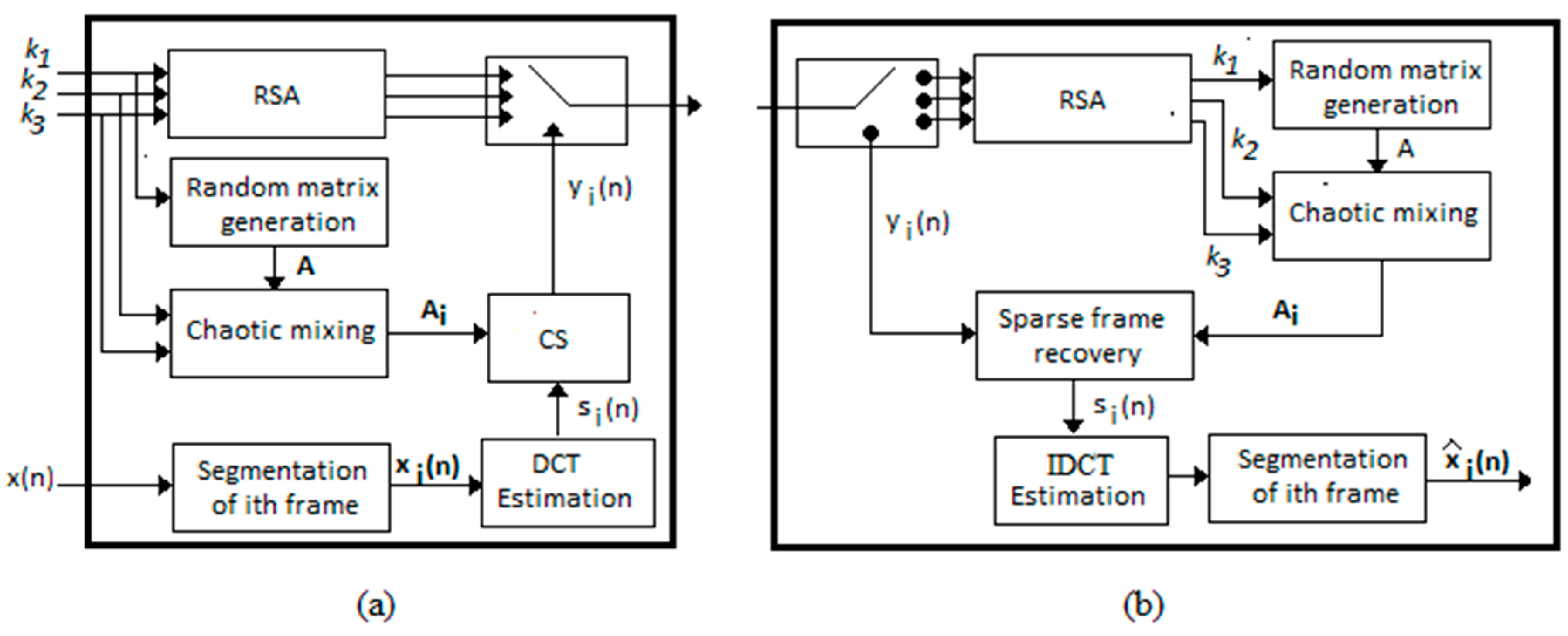
Figure 1.
Proposed encryption/des-encryption system. (a) Encryption and compression stage, (b) des-encryption and decompression stage. DCT, Discrete Cosine Transform; IDCT, Inverse DCT; CS, Compressive Sensing; RSA, Rivest, Shamir, and Adleman.
Figure 1.
Proposed encryption/des-encryption system. (a) Encryption and compression stage, (b) des-encryption and decompression stage. DCT, Discrete Cosine Transform; IDCT, Inverse DCT; CS, Compressive Sensing; RSA, Rivest, Shamir, and Adleman.
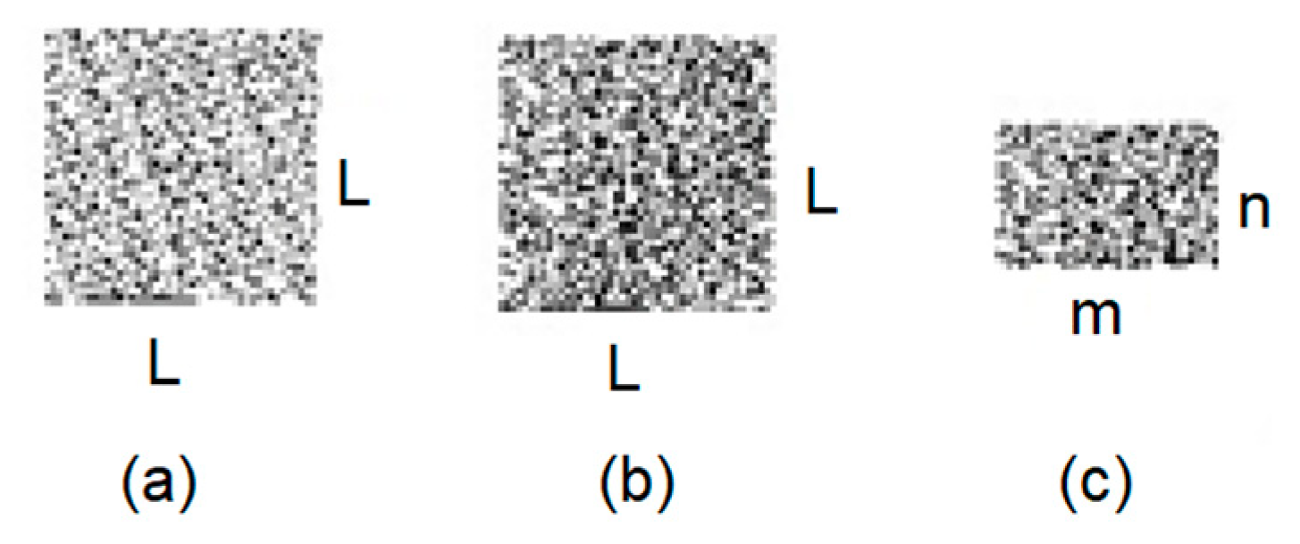
Figure 2.
Generation of matrix , using chaotic mixing. (a) Matrix A during frame j − 1, (b) matrix A during frame j, and (c) matrix during frame j.
Figure 2.
Generation of matrix , using chaotic mixing. (a) Matrix A during frame j − 1, (b) matrix A during frame j, and (c) matrix during frame j.
Figure 3.
(a). Original violin signal with a bit rate of 704 kb/s. (b). Decoded violin signal using the same sensing matrix during the encoding process with a bit rate of 704 kb/s. (c). Decoded violin signal using different sensing matrixes when the encoding and decoding processes are different, with a bit rate of 704 kb/s. (d). Decoded violin signal using the same sensing matrix during the encoding process with a bit rate of 176 kb/s. (e). Decoded violin signal using different sensing matrix during the encoding and decoding processes, with a bit rate of 176 kb/s. (f). Original popular music segment with a bit rate of 704 kb/s. (g). Decoded popular signal using the same sensing matrix during the encoding and decoding process with a bit rate of 352 kb/s. (h). Decoded popular signal using the different sensing matrix during the encoding and decoding process with a bit rate of 352 kb/s.
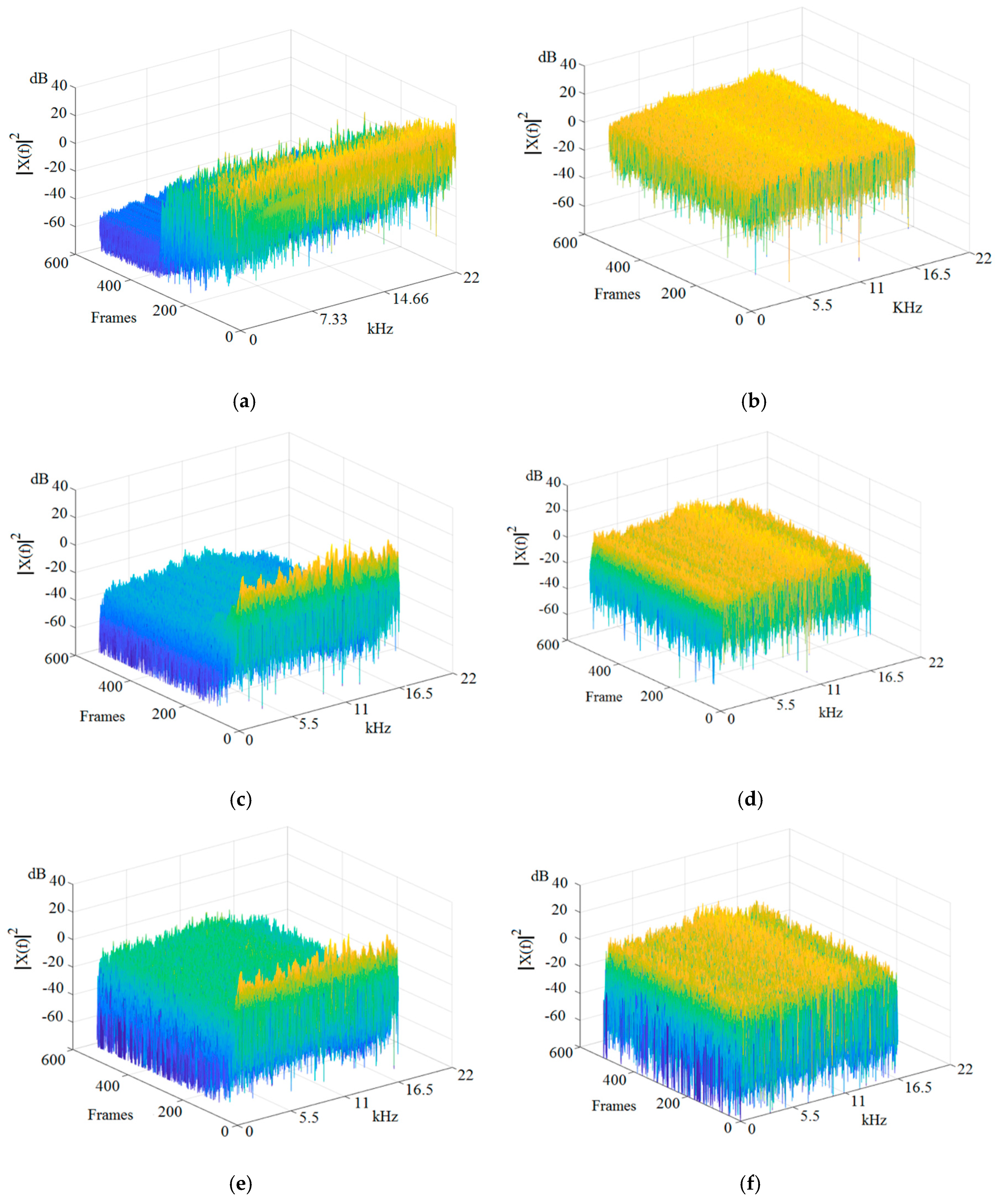
Figure 4.
(a). Spectrogram of a music signal obtained from a Bach concert with a bit rate of 704 kb/s. (b). Spectrogram of a encrypted music Bach violin signal with a bit rate of 704 kb/s. (c). Spectrogram of a decoded signal obtained using the same sensing matrix for encoding and decoding process with a bit rate of 176 kb/s. (d). Spectrogram of a decoded signal obtained using different sensing matrixes during the encoding and decoding process with a bit rate of 176 kb/s. (e). Spectrogram of a decoded signal obtained using the same sensing matrix for encoding and decoding process with a bit rate of 176 kb/s. (f). Spectrogram of a decoded signal obtained using different sensing matrixes during the encoding and decoding process with a bit rate of 176 kb/s.
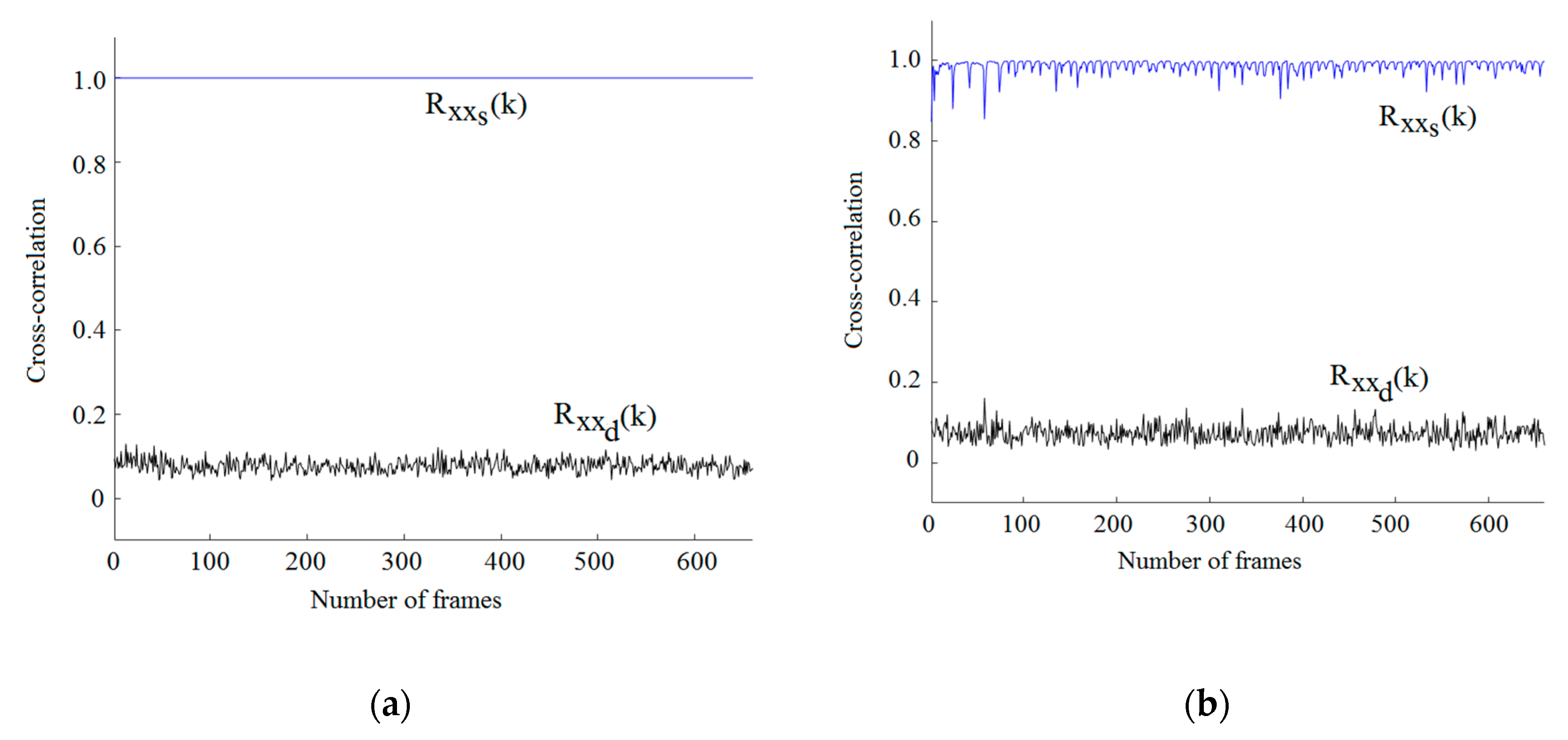
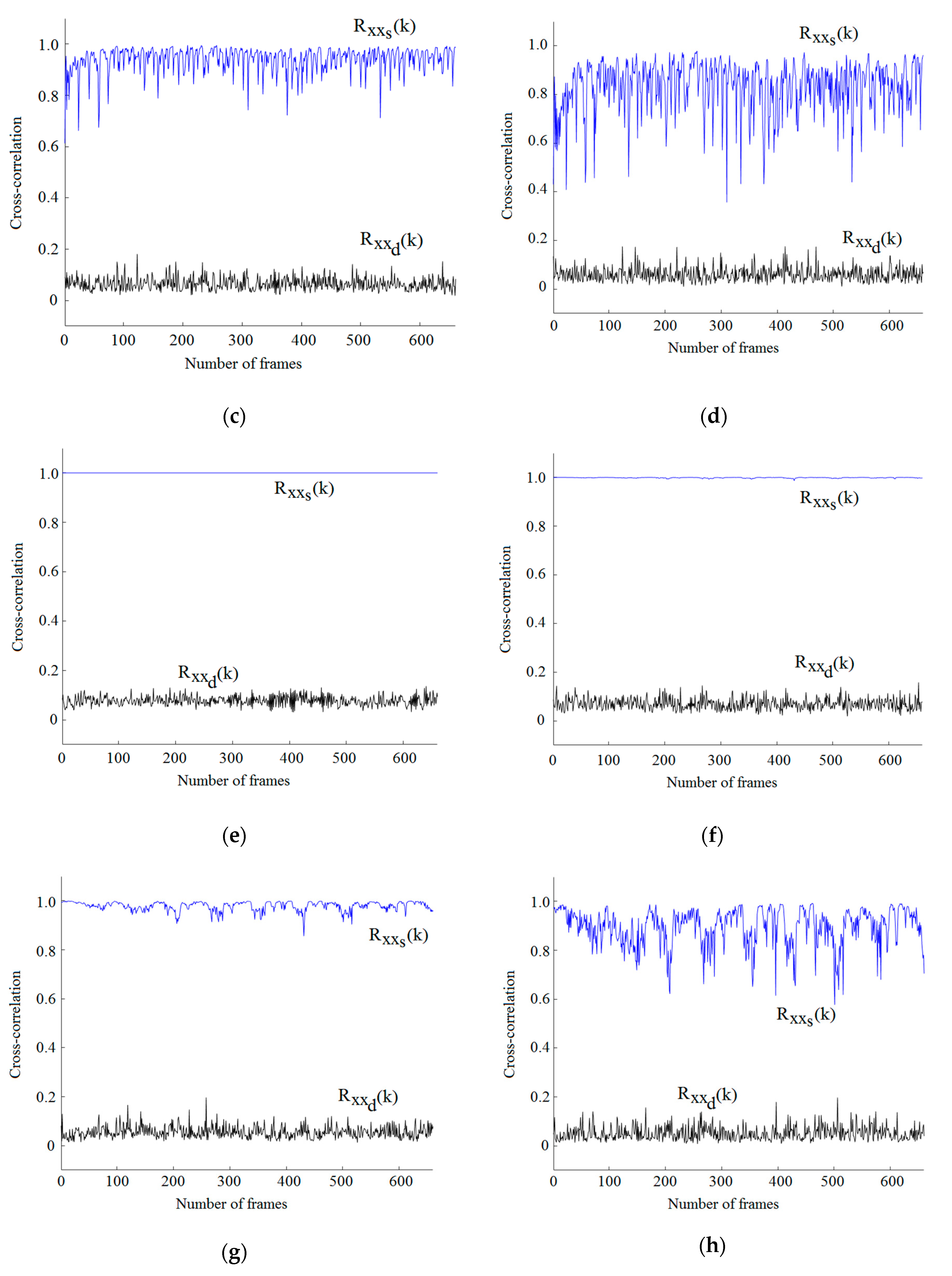
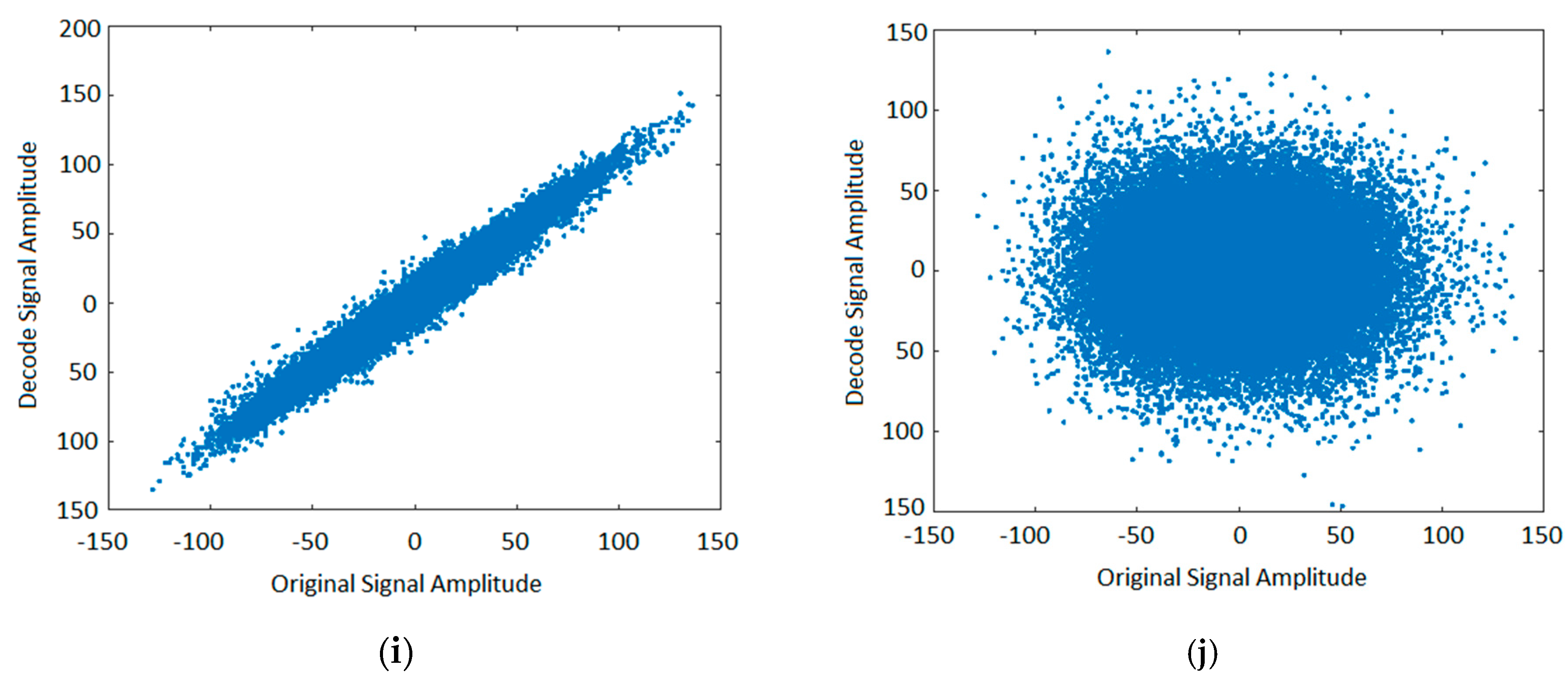
Figure 5.
(a). Correlation coefficient of popular music using the same, as well as a different sensing matrix, with 704 kb/s. (b). Correlation coefficient when popular music is decoded using the same, as well as a different sensing matrix, with 352 kb/s. (c). Correlation coefficient of popular music using the same, as well as a different sensing matrix, with 176 kb/s. (d). Correlation coefficient when popular music is decoded using the same, as well as a different sensing matrix, with 88 kb/s. (e). Correlation coefficient when classic music is decoded using the same, as well as a different sensing matrix, with 704 kb/s. (f). Correlation coefficient when classic music is decoded using the same, as well as a different sensing matrix, with 352 kb/s. (g). Correlation coefficient when classic music is decoded using the same, as well as a different sensing matrix, with 176 kb/s. (h). Correlation coefficient when classic music is decoded using the same, as well as a different sensing matrix, with 88 kb/s. (i). Dispersion diagram of the encoded and decoded signal when the same sensing matrix is used for encoding and decoding popular audio music. (j). Dispersion diagram of the encoded and decoded signal when different sensing matrixes are used for encoding and decoding a music signal.
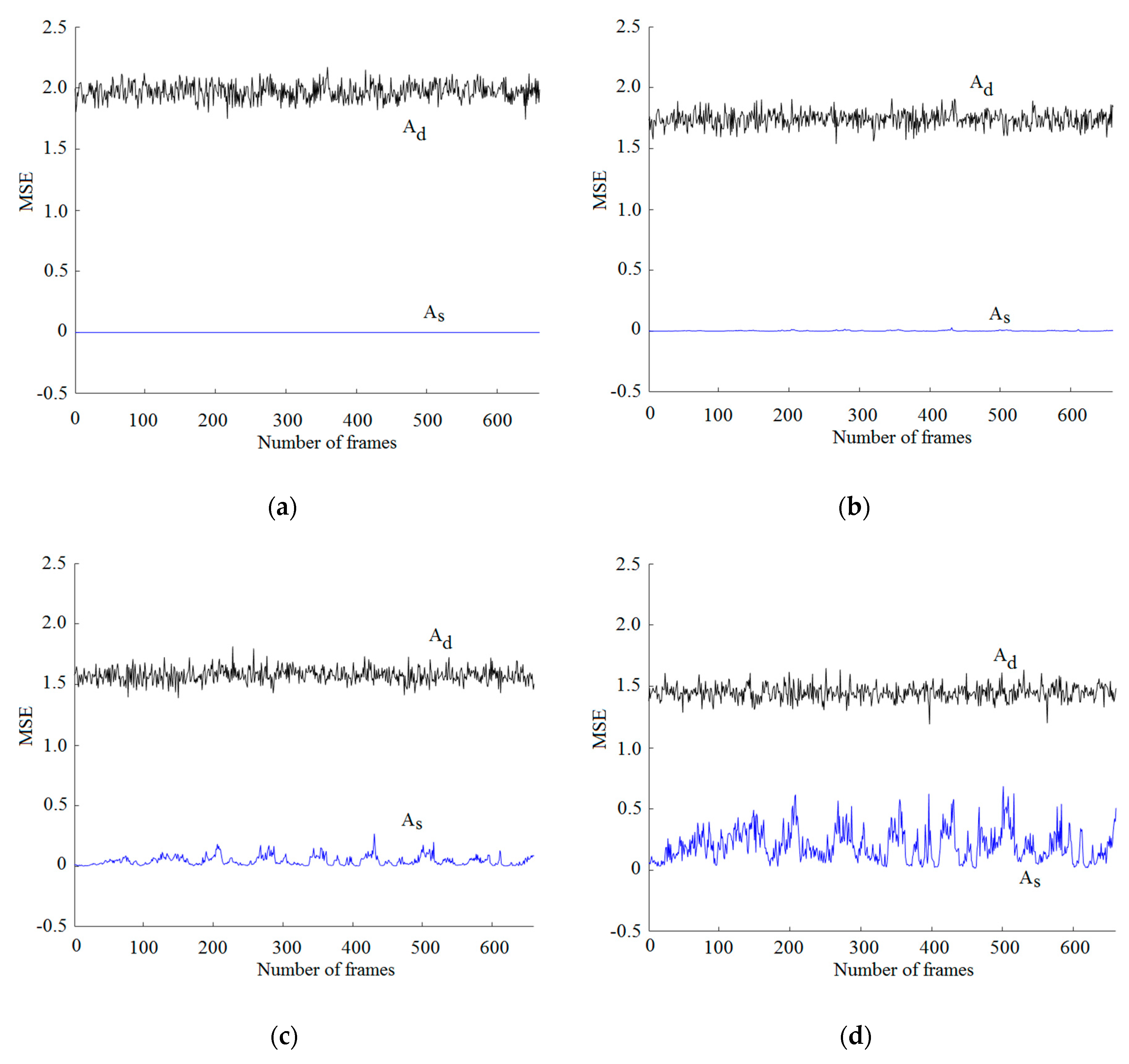
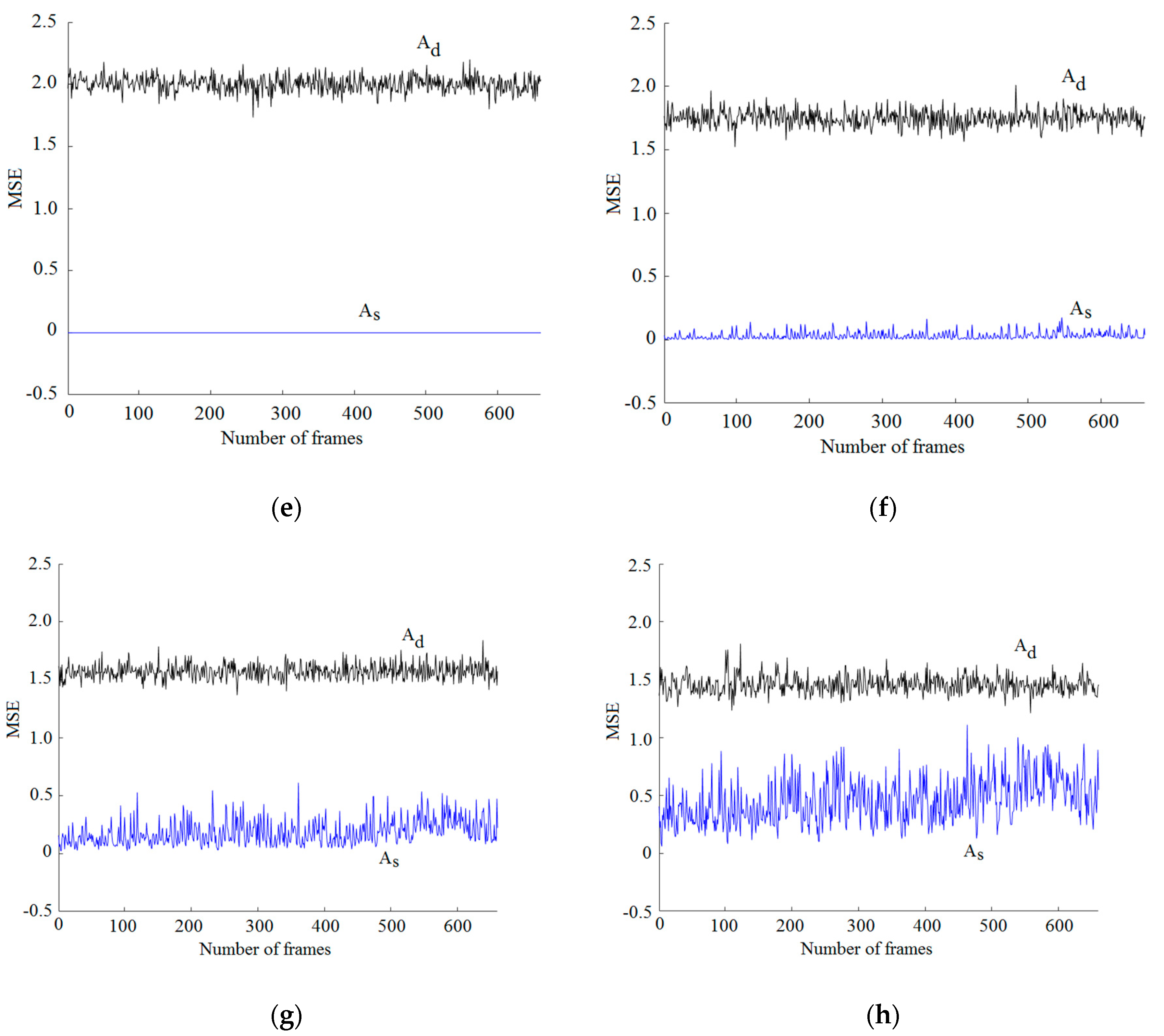
Figure 6.
(a) Mean square error (MSE) estimated when classic music, with a bit rate of 704 kb/s, is decoded using the same, As, and different, Ad, sensing matrix. (b) MSE obtained when classic music, with a bit rate of 352 kb/s, is decoded using the same, As, and different, Ad, sensing matrix. (c) MSE obtained when classic music with a bit rate of 176 kb/s is decoded using the same, As, and different, Ad, sensing matrix. (d) MSE obtained when classic music, with a bit rate of 88 kb/s, is decoded using the same, As, and different sensing matrix. (e) MSE using the same, As, and different, Ad, sensing matrix with a bit rate of 704 kb/s. (f) MSE using the same, As, and different, Ad, sensing matrix with a bit rate of 352 kb/s. (g) MSE using the same, As, and different, Ad, sensing matrix with a bit rate of 176 kb/s. (h) MSE using the same, As, and different, Ad, sensing matrix with a bit rate of 88 kb/s.
Figure 7.
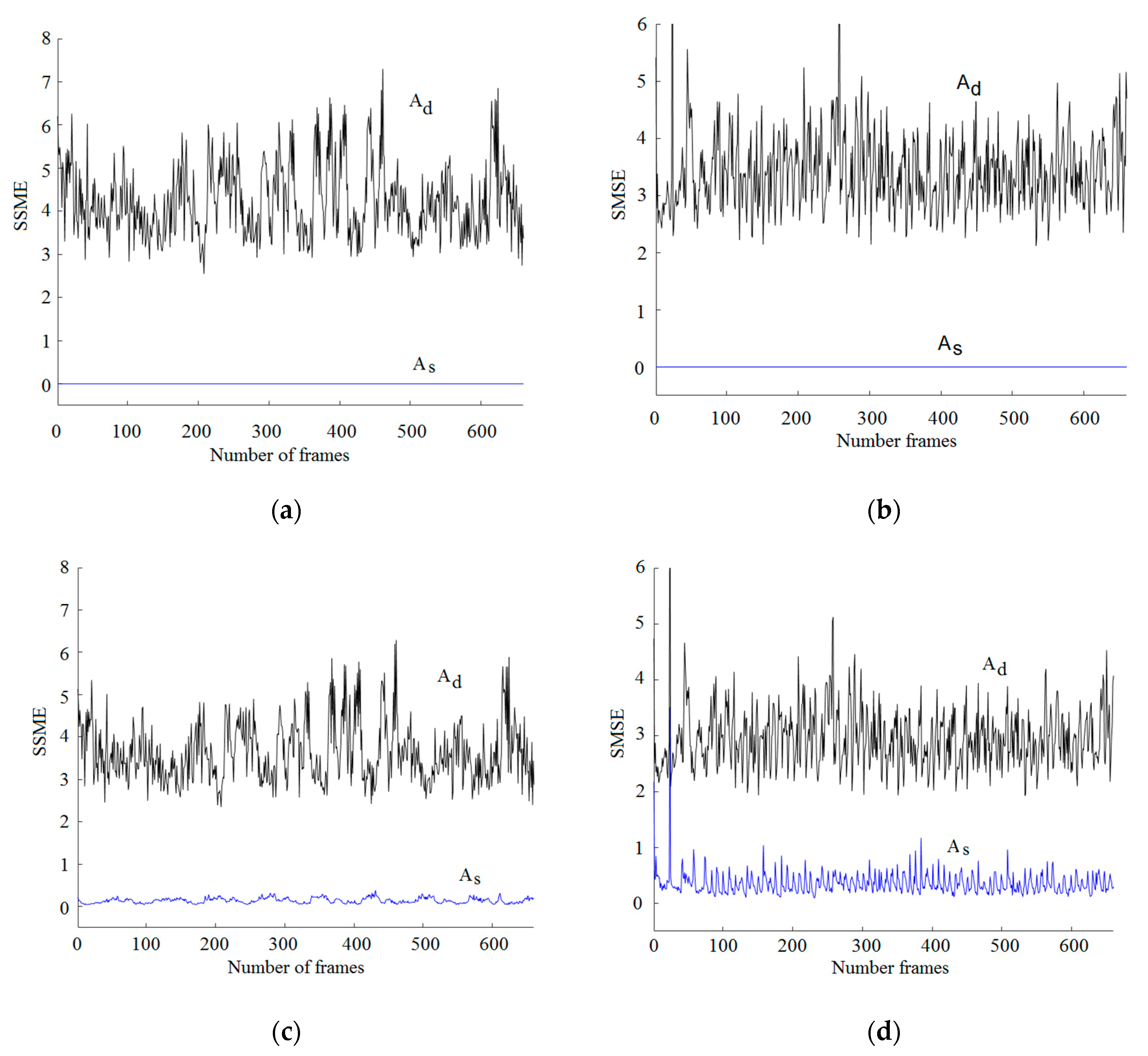
(a) Spectral similarity (SMSE) obtained when classic music is decoded using the same sensing matrix, with a sampling rate of 704 kb/s. (b) Spectral similarity (SMSE) obtained when classic music is decoded using the same sensing matrix, with a sampling rate of 352 kb/s. (c) Spectral similarity (SMSE) obtained when classic music is decoded using the same sensing matrix, with a sampling rate of 176 kb/s. (d) Spectral similarity (SMSE) obtained when classic music is decoded using the same sensing matrix, with a sampling rate of 88 kb/s.
Figure 7.
(a) Spectral similarity (SMSE) obtained when classic music is decoded using the same sensing matrix, with a sampling rate of 704 kb/s. (b) Spectral similarity (SMSE) obtained when classic music is decoded using the same sensing matrix, with a sampling rate of 352 kb/s. (c) Spectral similarity (SMSE) obtained when classic music is decoded using the same sensing matrix, with a sampling rate of 176 kb/s. (d) Spectral similarity (SMSE) obtained when classic music is decoded using the same sensing matrix, with a sampling rate of 88 kb/s.
Table 1.
Similarity, spectral similarity, and Person correlation obtained using the proposed system when popular music is encoded using a different number of samples/frames. MSE, mean square error; SMSE, spectral similarity.
Table 1.
Similarity, spectral similarity, and Person correlation obtained using the proposed system when popular music is encoded using a different number of samples/frames. MSE, mean square error; SMSE, spectral similarity.
| Samples/Frame | MSE | SMSE | Pearson-Correlation | kb/s |
|---|
| Same Matrix | Different Matrix | Same Matrix | Different Matrix | Same Matrix | Different Matrix |
|---|
| 128 | 0.4723 | 1.452 | 1.0219 | 2.1325 | 0.8636 | 0.0605 | 88 |
| 256 | 0.1920 | 1.539 | 0.7180 | 2.5095 | 0.9409 | 0.0651 | 176 |
| 512 | 0.0333 | 1.744 | 0.3524 | 2.9474 | 0.9872 | 0.0730 | 352 |
| 700 | 2 × 10⁻⁶ | 2.003 | 0.1696 | 3.1471 | 0.9968 | 0.0731 | 492 |
| 1024 | 2 × 10⁻⁶ | 2.003 | 1.1 × 10⁻⁶ | 3.4118 | 1.0000 | 0.0774 | 704 |
Table 2.
Similarity spectral similarity and Person correlation provided by the proposed system when classic music is encoded using a different number of samples/frames.
Table 2.
Similarity spectral similarity and Person correlation provided by the proposed system when classic music is encoded using a different number of samples/frames.
| Samples/Frame | MSE | SMSE | Pearson-Correlation | kb/s |
|---|
| Same Matrix | Different Matrix | Same Matrix | Different Matrix | Same Matrix | Different Matrix |
|---|
| 128 | 0.2863 | 1.458 | 0.9343 | 2.5923 | 0.8952 | 0.0510 | 88 |
| 256 | 0.1114 | 1.579 | 0.4949 | 3.0590 | 0.9787 | 0.0530 | 176 |
| 512 | 0.0260 | 1.744 | 0.1394 | 3.6377 | 0.9978 | 0.0700 | 352 |
| 700 | 0.0066 | 1.846 | 0.0623 | 3.9016 | 0.9987 | 0.0699 | 492 |
| 1024 | 4 × 10⁻⁶ | 1.994 | 4.7 × 10⁻⁶ | 4.2401 | 1.0000 | 0.0778 | 704 |
Table 3.
UACI and NSCR obtained using the proposed algorithm.
Table 3.
UACI and NSCR obtained using the proposed algorithm.
| Type | 704 kb/s | 352 kb/s | 176 kb/s |
|---|
| UACI | NSCR | UACI | NSCR | UACI | NSCR |
|---|
| Speech | 31.91 | 99.02 | 34.60 | 99.02 | 32.36 | 99.20 |
| Classic music | 29.32 | 98.96 | 29.32 | 98.05 | 33.70 | 98.98 |
| Popular music | 32.54 | 99.09 | 39.13 | 99.03 | 33.70 | 99.06 |
| Pop music | 35.05 | 99.88 | 39.16 | 99.12 | 32.54 | 99.03 |
Table 4.
Person correlation coefficient obtained using the proposed system and those proposed by G. Sudhish et al. [
3], Kordov [
25], and Sathiyamurthi [
24], with a bit rate of 704 kb/s.
Table 4.
Person correlation coefficient obtained using the proposed system and those proposed by G. Sudhish et al. [
3], Kordov [
25], and Sathiyamurthi [
24], with a bit rate of 704 kb/s.
| Scheme | Proposed | Ref. [7] | Ref. [25] | Ref. [24] |
|---|
| Classic | Popular | Classic | Popular | Classic | Popular | Classic | Popular |
|---|
| Same matrix | 0.9999 | 0.9999 | 0.9998 | 0.9998 | 0.9997 | 0.9998 | 0.9999 | 0.9999 |
| Different matrix | 0.0774 | 0.0778 | 0.0004 | 0.0003 | 0.0169 | 0.0048 | 0.0384 | 0.0157 |
Table 5.
Mean square error obtained using the proposed system and those proposed by G. Sudhish et al. [
3], Kordov [
25], and Sathiyamurthi [
24], with a bit rate of 704 kb/s.
Table 5.
Mean square error obtained using the proposed system and those proposed by G. Sudhish et al. [
3], Kordov [
25], and Sathiyamurthi [
24], with a bit rate of 704 kb/s.
| Scheme | Proposed (dB) | Ref. [3] (dB) | Ref. [25] (dB) | Ref. [24] (dB) |
|---|
| Classic | Popular | Classic | Popular | Classic | Popular | Classic | Popular |
|---|
| Same matrix | −53.27 | −53.27 | −31.308 | −31.302 | −20.655 | −26.193 | −32.596 | −33.098 |
| Different matrix | 6.2738 | 5.3298 | 2.2713 | 2.7717 | 5.8798 | 6.4667 | 2.4294 | 2.2632 |
Table 6.
Pearson-correlation coefficient and mean square error obtained using the proposed system and the system proposed by G. Sudhish et al. [
3], with bit rates of 352 kb/s and 176 kb/s.
Table 6.
Pearson-correlation coefficient and mean square error obtained using the proposed system and the system proposed by G. Sudhish et al. [
3], with bit rates of 352 kb/s and 176 kb/s.
| Scheme | Proposed | Sudhish et al. [3] | |
|---|
| Correlation | MSE (dB) | Correlation | MSE (dB) | Bit Rate |
|---|
| Classic | Popular | Classic | Popular | Classic | Popular | Classic | Popular | kb/s |
|---|
| Same matrix | 0.9978 | 0.9872 | −15.850 | −14.775 | 0.9989 | 0.0044 | −26.383 | −21.307 | 352 |
| Different matrix | 0.0730 | 0.0530 | 5.6083 | 2.4165 | 0.9971 | 0.0043 | 2.0798 | 2.3970 | 352 |
| Same matrix | 0.9787 | 0.0530 | −7.1670 | −9.5311 | 0.9940 | 0.0015 | −19.066 | −16.778 | 176 |
| Different matrix | 0.0530 | 0.0651 | 1.9841 | 1.8730 | 0.9898 | 0.0010 | 2.0548 | 2.4157 | 176 |
Table 7.
NSCR and UACI parameters obtained using the proposed system, and the systems proposed by G. Kordov [
25] and Sathiyamurthi [
24] with a bit rate of 704 kb/s.
Table 7.
NSCR and UACI parameters obtained using the proposed system, and the systems proposed by G. Kordov [
25] and Sathiyamurthi [
24] with a bit rate of 704 kb/s.
| Audio Signal | Proposed | Ref. [25] | Ref. [24] |
|---|
| | NSCR | UACI | NSCR | UACI | NSCR |
|---|
| Speech | 99.02% | 31.09% | 99.24% | 33.30% | 99.99% |
| Classical | 98.02% | 29.52% | 99.22% | 33.26% | 99.94% |
| Popular | 99.09% | 32.54% | 99.08% | 37.10% | 99.72% |

 and
and 


