Optimization of Public Transport Services to Minimize Passengers’ Waiting Times and Maximize Vehicles’ Occupancy Ratios


Abstract
:1. Introduction
2. State-of-the-Art
3. Problem Statement
4. Proposed Model
- Departure time of the vehicle from station i ;
- Vehicle assignment— the vehicle v of service s with given capacity c.
4.1. Assumptions, Variables, Parameters Which Are Time Dependent
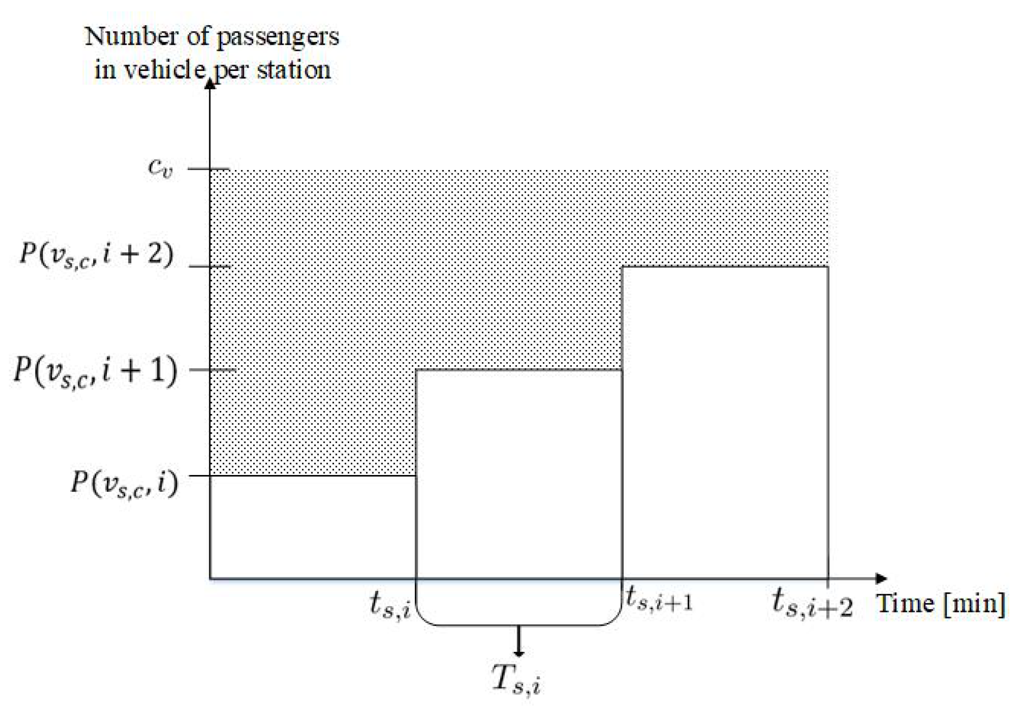
4.2. Assumptions, Variables, Parameters and Sets—Passengers, PWT and VOR
4.3. Objective Function
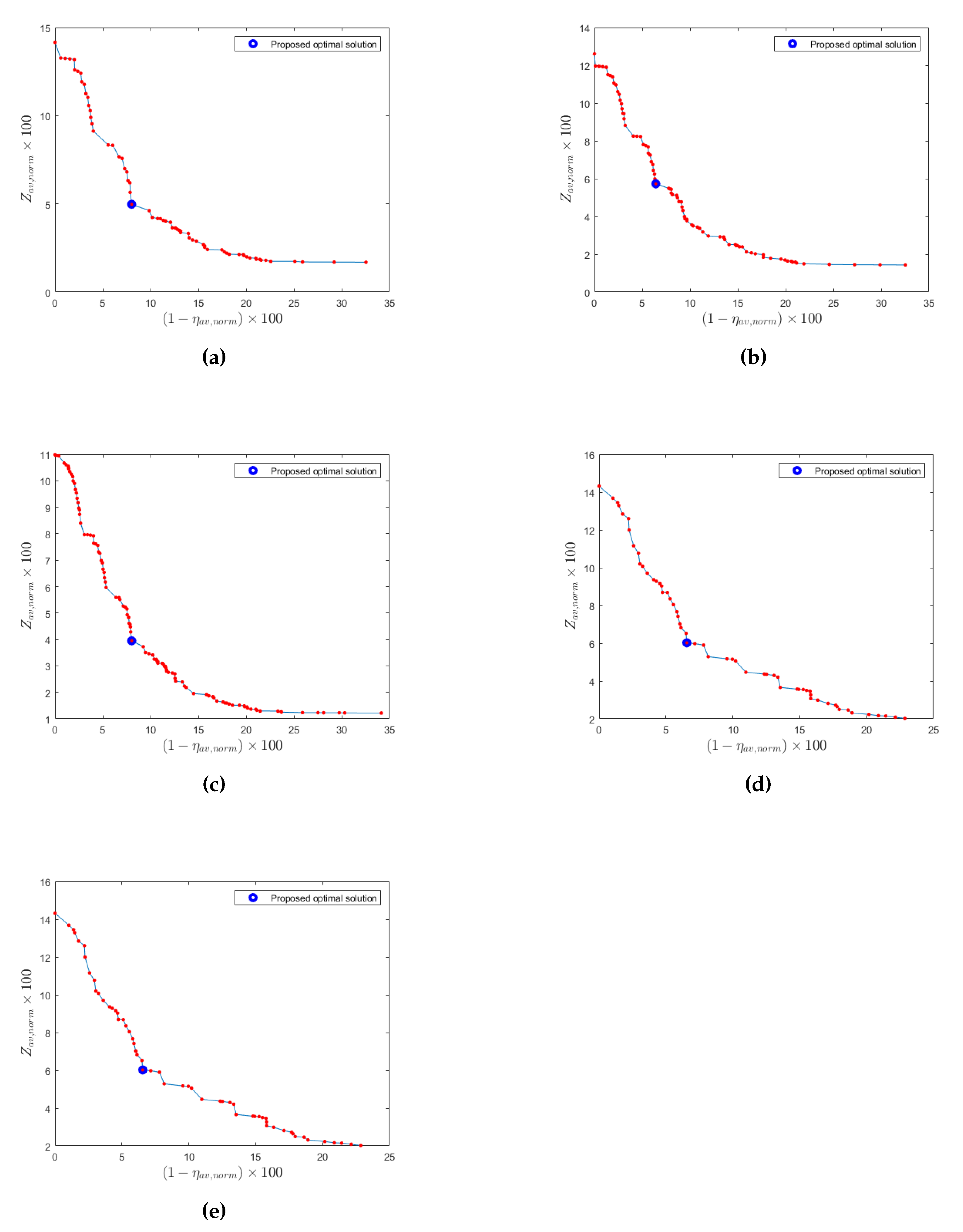
5. Results
5.1. Experiment 1
- Desired occupancy of each vehicle: 70;
- Possible departure time (in minutes) at the first terminal is defined by the time intervals for each service respectively:
- -
- -
- -
- .
5.2. Experiment 2
6. Analysis and Discussion
7. Conclusions
Author Contributions
Funding
Conflicts of Interest
Abbreviations
| PT | Public transportation |
| PSO | Particle swarm optimization |
| PWT | Passenger waiting time |
| VOR | Vehicles’ occupancy ratio |
| TTP | Train timetabling problem |
| WT | Waiting time |
| MOPSO | Multiobjective particle swarm optimization |
| GA | Genetic algorithm |
| TSP | Timetable synchronization problem |
| B&B | Branch and bound |
| OHM | Optimization based heuristic method |
| MIP | Mixed integer programming |
| PRTS | Periodic railway timetable scheduling problem |
| DE | Differential evolution |
| HPSO | Hybrid method of traditional PSO |
| OD | Origin-destination |
| TOPSIS | Technique for order of preference by similarity to ideal solution |
| AH | Average headway |
| EWT | Expected waiting time |
References
- Ceder, A. Bus frequency determination using passenger count data. Transp. Res. Part A General 1984, 18, 439–453. [Google Scholar] [CrossRef]
- Ceder, A.; Wilson, N.H. Bus network design. Transp. Res. Part B Methodol. 1986, 20, 331–344. [Google Scholar] [CrossRef]
- Ceder, A. Methods for creating bus timetables. Transp. Res. Part A General 1987, 21, 59–83. [Google Scholar] [CrossRef]
- Isaai, M.T.; Singh, M.G. Hybrid applications of constraint satisfaction and meta-heuristics to railway timetabling: A comparative study. IEEE Trans. Syst. Man Cybern. Part C (Appl. Rev.) 2001, 31, 87–95. [Google Scholar] [CrossRef]
- ShangGuan, W.; Yan, X.H.; Cai, B.G.; Wang, J. Multiobjective optimization for train speed trajectory in CTCS high-speed railway with hybrid evolutionary algorithm. IEEE Trans. Intell. Transp. Syst. 2015, 16, 2215–2225. [Google Scholar] [CrossRef]
- Park, Y.B. A hybrid genetic algorithm for the vehicle scheduling problem with due times and time deadlines. Int. J. Prod. Econ. 2001, 73, 175–188. [Google Scholar] [CrossRef]
- Caprara, A.; Fischetti, M.; Toth, P. Modeling and solving the train timetabling problem. Oper. Res. 2002, 50, 851–861. [Google Scholar] [CrossRef]
- Siebert, M.; Goerigk, M. An experimental comparison of periodic timetabling models. Comput. Oper. Res. 2013, 40, 2251–2259. [Google Scholar] [CrossRef]
- Shafia, M.A.; Sadjadi, S.J.; Jamili, A.; Tavakkoli-Moghaddam, R.; Pourseyed-Aghaee, M. The periodicity and robustness in a single-track train scheduling problem. Appl. Soft Comput. 2012, 12, 440–452. [Google Scholar] [CrossRef]
- Bussieck, M.R.; Kreuzer, P.; Zimmermann, U.T. Optimal lines for railway systems. Eur. J. Oper. Res. 1997, 96, 54–63. [Google Scholar] [CrossRef]
- Yalcınkaya, Ö.; Bayhan, G.M. Modelling and optimization of average travel time for a metro line by simulation and response surface methodology. Eur. J. Oper. Res. 2009, 196, 225–233. [Google Scholar] [CrossRef]
- Ceder, A. Public Transit Planning and Operation: Modeling, Practice and Behavior; CRC Press: Boca Raton, FL, USA, 2016. [Google Scholar]
- Chang, S.J.; Hsu, S.C. Modeling of passenger waiting time in intermodal station with constrained capacity on intercity transit. Int. J. Urban Sci. 2004, 8, 51–60. [Google Scholar] [CrossRef]
- Baita, F.; Pesenti, R.; Ukovich, W.; Favaretto, D. A comparison of different solution approaches to the vehicle scheduling problem in a practical case. Comput. Oper. Res. 2000, 27, 1249–1269. [Google Scholar] [CrossRef]
- Hassold, S.; Ceder, A. Multiobjective approach to creating bus timetables with multiple vehicle types. Transp. Res. Rec. 2012, 2276, 56–62. [Google Scholar] [CrossRef]
- Hassold, S.; Ceder, A. Public transport vehicle scheduling featuring multiple vehicle types. Transp. Res. Part B Methodol. 2014, 67, 129–143. [Google Scholar] [CrossRef]
- Wang, Y.; Tang, T.; Ning, B.; van den Boom, T.J.; De Schutter, B. Passenger-demands-oriented train scheduling for an urban rail transit network. Transp. Res. Part C Emerg. Technol. 2015, 60, 1–23. [Google Scholar] [CrossRef]
- Sun, H.; Wu, J.; Ma, H.; Yang, X.; Gao, Z. A Bi-Objective Timetable Optimization Model for Urban Rail Transit Based on the Time-Dependent Passenger Volume. IEEE Trans. Intell. Transp. Syst. 2019, 20, 604–615. [Google Scholar] [CrossRef]
- Wong, R.C.W.; Yuen, T.W.Y.; Fung, K.W.; Leung, J.M.Y. Optimizing Timetable Synchronization for Rail Mass Transit. Transp. Sci. 2008, 42, 57–69. [Google Scholar] [CrossRef]
- Wu, Y.; Tang, J.; Yu, Y.; Pan, Z. A stochastic optimization model for transit network timetable design to mitigate the randomness of traveling time by adding slack time. Transp. Res. Part C Emerg. Technol. 2015, 52, 15–31. [Google Scholar] [CrossRef]
- Wu, J.; Liu, M.; Sun, H.; Li, T.; Gao, Z.; Wang, D.Z. Equity-based timetable synchronization optimization in urban subway network. Transp. Res. Part C Emerg. Technol. 2015, 51, 1–18. [Google Scholar] [CrossRef]
- Shafahi, Y.; Khani, A. A practical model for transfer optimization in a transit network: Model formulations and solutions. Transp. Res. Part A Policy Pract. 2010, 44, 377–389. [Google Scholar] [CrossRef]
- Liu, T.; Ceder, A.A. Integrated public transport timetable synchronization and vehicle scheduling with demand assignment: A bi-objective bi-level model using deficit function approach. Transp. Res. Part B Methodol. 2018, 117, 935–955. [Google Scholar] [CrossRef]
- Zhong, J.H.; Shen, M.; Zhang, J.; Chung, H.S.H.; Shi, Y.H.; Li, Y. A differential evolution algorithm with dual populations for solving periodic railway timetable scheduling problem. IEEE Trans. Evolut. Comput. 2012, 17, 512–527. [Google Scholar] [CrossRef]
- Niu, H.; Zhang, M. An optimization to schedule train operations with phase-regular framework for intercity rail lines. Discret. Dyn. Nat. Soc. 2012, 2012. [Google Scholar] [CrossRef]
- Barrena, E.; Canca, D.; Coelho, L.C.; Laporte, G. Exact formulations and algorithm for the train timetabling problem with dynamic demand. Comput. Oper. Res. 2014, 44, 66–74. [Google Scholar] [CrossRef]
- Barrena, E.; Canca, D.; Coelho, L.C.; Laporte, G. Single-line rail rapid transit timetabling under dynamic passenger demand. Transp. Res. Part B Methodol. 2014, 70, 134–150. [Google Scholar] [CrossRef]
- Vansteenwegen, P.; Van Oudheusden, D. Developing railway timetables which guarantee a better service. Eur. J. Oper. Res. 2006, 173, 337–350. [Google Scholar] [CrossRef]
- Vansteenwegen, P.; Van Oudheusden, D. Decreasing the passenger waiting time for an intercity rail network. Transp. Res. Part B Methodol. 2007, 41, 478–492. [Google Scholar] [CrossRef]
- Corman, F.; D’Ariano, A.; Pacciarelli, D.; Pranzo, M. Bi-objective conflict detection and resolution in railway traffic management. Transp. Res. Part C Emerg. Technol. 2012, 20, 79–94. [Google Scholar] [CrossRef]
- Parbo, J.; Nielsen, O.A.; Prato, C.G. User perspectives in public transport timetable optimisation. Transp. Res. Part C Emerg. Technol. 2014, 48, 269–284. [Google Scholar] [CrossRef] [Green Version]
- Berrebi, S.J.; Watkins, K.E.; Laval, J.A. A real-time bus dispatching policy to minimize passenger wait on a high frequency route. Transp. Res. Part B Methodol. 2015, 81, 377–389. [Google Scholar] [CrossRef]
- Li, J.; Hu, J.; Zhang, Y. Optimal combinations and variable departure intervals for micro bus system. Tsinghua Sci. Technol. 2017, 22, 282–292. [Google Scholar] [CrossRef]
- Hussain, B.; Khan, A.; Javaid, N.; Hasan, Q.U.; A Malik, S.; Ahmad, O.; Dar, A.H.; Kazmi, A. A Weighted-Sum PSO Algorithm for HEMS: A New Approach for the Design and Diversified Performance Analysis. Electronics 2019, 8, 180. [Google Scholar] [CrossRef] [Green Version]
- Zuo, X.; Li, B.; Huang, X.; Zhou, M.; Cheng, C.; Zhao, X.; Liu, Z. Optimizing hospital emergency department layout via multiobjective tabu search. IEEE Trans. Autom. Sci. Eng. 2019, 16, 1137–1147. [Google Scholar] [CrossRef]
- Wu, Q.; Zhou, M.; Zhu, Q.; Xia, Y.; Wen, J. MOELS: Multiobjective Evolutionary List Scheduling for Cloud Workflows. IEEE Trans. Autom. Sci. Eng. 2019, 17, 166–176. [Google Scholar] [CrossRef]
- Gao, K.; Cao, Z.; Zhang, L.; Chen, Z.; Han, Y.; Pan, Q. A review on swarm intelligence and evolutionary algorithms for solving flexible job shop scheduling problems. IEEE/CAA J. Autom. Sin. 2019, 6, 904–916. [Google Scholar] [CrossRef]
- Coello, C.A.C.; Pulido, G.T.; Lechuga, M.S. Handling multiple objectives with particle swarm optimization. IEEE Trans. Evol. Comput. 2004, 8, 256–279. [Google Scholar] [CrossRef]
- Lv, Z.; Wang, L.; Han, Z.; Zhao, J.; Wang, W. Surrogate-assisted particle swarm optimization algorithm with Pareto active learning for expensive multi-objective optimization. IEEE/CAA J. Autom. Sin. 2019, 6, 838–849. [Google Scholar] [CrossRef]
- Wang, Z.; Rangaiah, G.P. Application and analysis of methods for selecting an optimal solution from the Pareto-optimal front obtained by multiobjective optimization. Ind. Eng. Chem. Res. 2017, 56, 560–574. [Google Scholar] [CrossRef]


| Paper | Year | Objective | Constraints | Solution Method | Case |
|---|---|---|---|---|---|
| [28] | 2006 | Minimize the waiting time | Running time, departure time, buffer time, spacing time | Linear programming | real |
| [19] | 2008 | Minimize the interchange waiting times | Running time, dwell times, trip times, headways, turnaround | B&B, heuristic | real |
| [22] | 2010 | Minimize the waiting time | Headway bounds, extra dwell times | Genetic algorithm | real |
| [15] | 2012 | Minimize the expected passenger waiting time and Minimize the discrepancy from a desired occupancy level on the vehicles | Headway bounds, vehicle capacity | A multi-objective label-correcting algorithm | real |
| [25] | 2012 | Minimize the waiting time | Headway, in-train passengers, passenger demands, fleet-size, number of boarded passengers | Genetic algorithm | real |
| [24] | 2013 | Minimize the waiting time | Traveling time | Evolutionary algorithm | real |
| [31] | 2014 | Minimize the waiting time | Headway, departure time | Tabu Search algorithm | test |
| [17] | 2015 | Minimize the total travel time of all passengers and the energy consumption of the trains using a weighted sum strategy | Headway, train capacity | Evolutionary algorithms | test |
| [21] | 2015 | Minimize the maximal passenger waiting time | Headway, departure time, running time | Genetic algorithm | real |
| [32] | 2015 | Minimize the waiting time | Headway | Analytical | test |
| [33] | 2017 | Minimize the waiting time | Headway | Improvements of the Genetic Algorithm and Particle Swarm Optimization | test |
| [23] | 2018 | Vehicle scheduling problem with the transit assignment | Headway, the number of vehicle departures, fleet size | Heuristic | test |
| [18] | 2019 | Minimize the PWT and energy consumption | Headway | Genetic algorithm | real |
| This paper | Minimize the waiting time and maximize vehicles’ occupancy | Headway, passenger demands, number of boarded passengers | Particle swarm optimization | test |
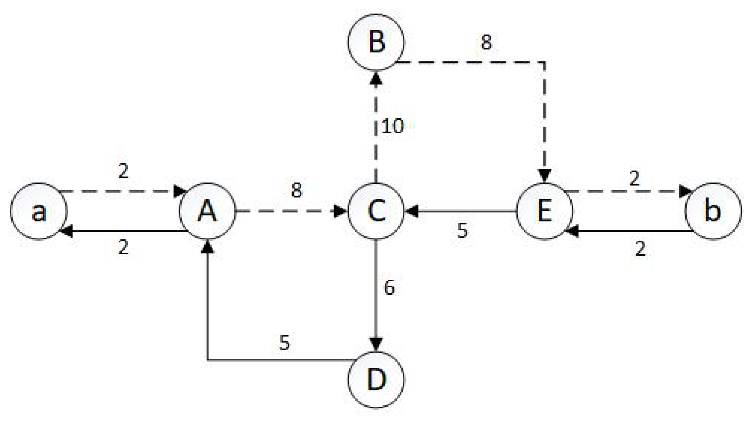
| From\To | A | B | C | D | E |
|---|---|---|---|---|---|
| A | 0 | 100 | 50 | 70 | 80 |
| B | 0 | 0 | 0 | 0 | 50 |
| C | 50 | 20 | 0 | 80 | 60 |
| D | 60 | 0 | 0 | 0 | 0 |
| E | 80 | 100 | 20 | 60 | 0 |
| GENERAL | |
| OD | Origin-destination |
| Set of OD pairs for a given service s | |
| Set of services for a given OD pair | |
| Set of vehicles | |
| Set of stations | |
| L | Set of lines |
| Vehicle v with capacity c, for service s | |
| INDEXES | |
| Service s from the set of services | |
| Station i from the set of stations | |
| Vehicle v from the set of vehicles | |
| Line l from the set of lines | |
| VARIABLES | |
| Departure time of the vehicle at station i for service s | |
| Arrival time of the vehicle at station i for service s | |
| Desired occupancy | |
| Dwelling time at station i for service s | |
| Running time – traveling time between adjacent | |
| stations i and for service s | |
| Sum of running time between all adjacent | |
| stations for service s | |
| Headway – difference between departure times at station i | |
| for consecutive services s and | |
| Difference between departure times of vehicle v | |
| between adjacent stations i and for a given service s | |
| Time horizon for i-th station | |
| Total number of passengers in vehicle v in station i | |
| Number of passengers entering the vehicle in station i | |
| heading for destination j ( OD pair) | |
| Number of passengers who entered the vehicle | |
| in station k with traveling to j | |
| Number of passengers exiting vehicle v of service s at station i | |
| Number of passengers entering vehicle v of service s at station i | |
| Number of passengers in vehicle v of service s arriving at station i | |
| Number of passengers remaining at station i | |
| after vehicle v of service s leaves the station | |
| Average waiting time at station i | |
| Average number of passengers per time | |
| Amount of PWT at station i for service s | |
| Total vehicles’ occupancy ratio for all services for a given line | |
| Average vehicle occupancy ratio for service s |
| Dep. Time | Number of Passengers Left at the Station | Waiting Time | Amount of PWT (Equation (11)) | ||||||||||
|---|---|---|---|---|---|---|---|---|---|---|---|---|---|
| q = 4 | Proposed method | [7:15, 7:28, 7:38, 7:46] | 0.142 | 230 | 152 | 8 | 13 | 12 | 12 | 4386.45 | 2813.87 | 336.74 | |
| 460 | 304 | 16 | 10 | 9 | 9 | 5674.19 | 3684.52 | 339.03 | |||||
| 690 | 456 | 24 | 8 | 7 | 7 | 6379.35 | 4163.61 | 335.23 | |||||
| 920 | 608 | 32 | 90 | 89 | 89 | 92,467.74 | 60,520.65 | 4491.29 | |||||
| Results according to [23] | [7:15, 7:30, 7:45, 8:00] | 0.161 | 230 | 152 | 8 | 15 | 14 | 14 | 5700 | 3630 | 495 | ||
| 460 | 304 | 16 | 15 | 14 | 14 | 9150 | 5910 | 615 | |||||
| 690 | 456 | 24 | 15 | 14 | 14 | 12,600 | 8190 | 735 | |||||
| 920 | 608 | 32 | 90 | 89 | 89 | 96,300 | 62,820 | 5130 | |||||
| q = 5 | Proposed method | [7:12, 7:24, 7:35, 7:43, 7:49] | 0.126 | 230 | 152 | 8 | 12 | 11 | 11 | 4239.73 | 2711.84 | 342.62 | |
| 460 | 304 | 16 | 11 | 10 | 10 | 6416.42 | 4157.85 | 402.07 | |||||
| 690 | 456 | 24 | 8 | 7 | 7 | 6506.49 | 4239.89 | 356.41 | |||||
| 920 | 608 | 32 | 6 | 5 | 5 | 6259.86 | 4091.92 | 315.31 | |||||
| 1150 | 760 | 40 | 72 | 71 | 71 | 91,678.38 | 60,047.03 | 4359.73 | |||||
| Results according to [23] | [7:12, 7:24, 7:36, 7:48, 8:00] | 0.141 | 230 | 152 | 8 | 12 | 11 | 11 | 4560 | 2904 | 396 | ||
| 460 | 304 | 16 | 12 | 11 | 11 | 7320 | 4728 | 492 | |||||
| 690 | 456 | 24 | 12 | 11 | 11 | 10,080 | 6552 | 588 | |||||
| 920 | 608 | 32 | 12 | 11 | 11 | 12,840 | 8376 | 684 | |||||
| 1150 | 760 | 40 | 72 | 71 | 71 | 93,600 | 61,200 | 4680 | |||||
| q = 6 | Proposed method | [7:10, 7:20, 7:30, 7:40, 7:47, 7:51] | 0.114 | 230 | 152 | 8 | 10 | 9 | 9 | 3635.37 | 2321.22 | 302.56 | |
| 460 | 304 | 16 | 10 | 9 | 9 | 5935.37 | 3841.22 | 382.56 | |||||
| 690 | 456 | 24 | 10 | 9 | 9 | 8235.37 | 5361.22 | 462.56 | |||||
| 920 | 608 | 32 | 7 | 6 | 6 | 7374.76 | 4816.85 | 379.79 | |||||
| 1150 | 760 | 40 | 4 | 3 | 3 | 5134.15 | 3360.49 | 249.02 | |||||
| 1380 | 912 | 48 | 60 | 59 | 59 | 90,812.20 | 59,527.32 | 4215.37 | |||||
| Results according to [23] | [7:10, 7:20, 7:30, 7:40, 7:50, 8:00] | 0.127 | 230 | 152 | 8 | 10 | 9 | 9 | 3800 | 2420 | 330 | ||
| 460 | 304 | 16 | 10 | 9 | 9 | 6100 | 3940 | 410 | |||||
| 690 | 456 | 24 | 10 | 9 | 9 | 8400 | 5460 | 490 | |||||
| 920 | 608 | 32 | 10 | 9 | 9 | 10,700 | 6980 | 570 | |||||
| 1150 | 760 | 40 | 10 | 9 | 9 | 13,000 | 8500 | 650 | |||||
| 1380 | 912 | 48 | 60 | 59 | 59 | 91,800 | 60,120 | 4380 | |||||
| q = 4 | Proposed method | [7:15, 7:28, 7:38, 7:46] | 0.169 | 190 | 178 | 21 | 13 | 12 | 12 | 3680.26 | 3291.52 | 552.29 | |
| 380 | 355 | 41 | 10 | 9 | 9 | 4730.97 | 4301.94 | 624.84 | |||||
| 570 | 533 | 62 | 8 | 7 | 7 | 5304.77 | 4865.55 | 667.87 | |||||
| 760 | 711 | 83 | 90 | 89 | 89 | 76,778.71 | 70,757.42 | 9403.55 | |||||
| Results according to [23] | [7:15, 7:30, 7:45, 8:00] | 0.192 | 190 | 178 | 21 | 15 | 14 | 14 | 4800 | 4245 | 765 | ||
| 380 | 355 | 41 | 15 | 14 | 14 | 7650 | 6900 | 1065 | |||||
| 570 | 533 | 62 | 15 | 14 | 14 | 10,500 | 9570 | 1380 | |||||
| 760 | 711 | 83 | 90 | 89 | 89 | 80,100 | 73,440 | 10,170 | |||||
| q = 5 | Proposed method | [7:12, 7:24, 7:35, 7:43, 7:49] | 0.150 | 190 | 178 | 21 | 12 | 11 | 11 | 3562.43 | 3171.81 | 547.95 | |
| 380 | 355 | 41 | 11 | 10 | 10 | 5355.56 | 4854.49 | 722.28 | |||||
| 570 | 533 | 62 | 8 | 7 | 7 | 5414.95 | 4954.54 | 693.30 | |||||
| 760 | 711 | 83 | 6 | 5 | 5 | 5201.22 | 4783.91 | 645.97 | |||||
| 950 | 888 | 103 | 72 | 71 | 71 | 76,094.59 | 70,150.86 | 9191.68 | |||||
| Results according to [23] | [7:12, 7:24, 7:36, 7:48, 8:00] | 0.168 | 190 | 178 | 21 | 12 | 11 | 11 | 3840 | 3396 | 612 | ||
| 380 | 355 | 41 | 12 | 11 | 11 | 6120 | 5520 | 852 | |||||
| 570 | 533 | 62 | 12 | 11 | 11 | 8400 | 7656 | 1104 | |||||
| 760 | 711 | 83 | 12 | 11 | 11 | 10,680 | 9792 | 1356 | |||||
| 950 | 888 | 103 | 72 | 71 | 71 | 77,760 | 71,496 | 9576 | |||||
| Vehicle Occupancy | Number of Free Seats | Number of Passengers Left at the Station | Waiting Time | Amount of PWT (Equation (11)) | ||||||||||||||||
|---|---|---|---|---|---|---|---|---|---|---|---|---|---|---|---|---|---|---|---|---|
| q = 4 | Dep. time | [7:15, 7:25, 7:37, 7:46] | 0.080 | 1 | 1 | 1 | 0 | 0 | 0 | 230 | 152 | 8 | 0.498 | 10 | 9 | 9 | 3348.39 | 2149.03 | 254.73 | |
| 1 | 1 | 0.52 | 0 | 0 | 236 | 40 | 136 | 0 | 12 | 11 | 0 | 1738.06 | 2386.84 | 209.68 | ||||||
| [70, 490, 70, 490] | 1 | 1 | 1 | 0 | 0 | 0 | 270 | 288 | 8 | 9 | 8 | 8 | 3373.55 | 3158.13 | 229.26 | |||||
| 1 | 1 | 0.52 | 0 | 0 | 236 | 80 | 272 | 0 | 90 | 89 | 0 | 16635.48 | 30141.29 | 1572.58 | ||||||
| q = 5 | Dep. time | [7:12, 7:21, 7:32, 7:40, 7:49] | 0.064 | 1 | 1 | 1 | 0 | 0 | 0 | 230 | 152 | 8 | 0.057 | 9 | 8 | 8 | 3125.07 | 2001.04 | 247.84 | |
| 1 | 1 | 0.52 | 0 | 0 | 236 | 40 | 136 | 0 | 11 | 10 | 0 | 1729.53 | 2269.72 | 214.92 | ||||||
| [70, 490, 70, 490, 350] | 1 | 1 | 1 | 0 | 0 | 0 | 270 | 288 | 8 | 8 | 7 | 7 | 3097.84 | 2866.7 | 220.31 | |||||
| 1 | 1 | 0.52 | 0 | 0 | 236 | 80 | 272 | 0 | 9 | 8 | 0 | 1775.07 | 3081.04 | 175.84 | ||||||
| 1 | 1 | 1 | 0 | 0 | 0 | 310 | 424 | 8 | 72 | 71 | 71 | 30760.54 | 35592.32 | 1982.76 | ||||||
| q = 6 | Dep. time | [7:10, 7:19, 7:29, 7:36, 7:45, 7:51] | 0.080 | 1 | 1 | 1 | 0 | 0 | 0 | 230 | 152 | 8 | 0.040 | 9 | 8 | 8 | 3245.49 | 2073.29 | 267.91 | |
| 1 | 1 | 0.52 | 0 | 0 | 236 | 40 | 136 | 0 | 10 | 9 | 0 | 1669.51 | 2121.71 | 211.59 | ||||||
| 1 | 1 | 1 | 0 | 0 | 0 | 270 | 288 | 8 | 7 | 6 | 6 | 2778.66 | 2549.20 | 204.11 | ||||||
| [70, 490, 70, 490, 70, 490] | 1 | 1 | 0.52 | 0 | 0 | 236 | 80 | 272 | 0 | 9 | 8 | 0 | 1862.56 | 3133.54 | 190.43 | |||||
| 1 | 1 | 1 | 0 | 0 | 0 | 310 | 424 | 8 | 6 | 5 | 5 | 2621.71 | 3001.02 | 174.95 | ||||||
| 1 | 1 | 0.52 | 0 | 0 | 236 | 120 | 408 | 0 | 60 | 59 | 0 | 14817.07 | 29050.24 | 1269.51 | ||||||
| q = 4 | Dep. time | [7:15, 7:25, 7:37, 7:46] | 0.066 | 1 | 1 | 1 | 0 | 0 | 0 | 190 | 178 | 21 | 0.060 | 10 | 9 | 9 | 2808.60 | 2513.87 | 419.68 | |
| 1 | 1 | 0.63 | 0 | 0 | 154 | 30 | 194 | 0 | 12 | 11 | 0 | 1450.32 | 3208.65 | 251.61 | ||||||
| [70, 420, 70, 490] | 1 | 1 | 1 | 0 | 0 | 0 | 220 | 371 | 20 | 9 | 8 | 8 | 2797.74 | 3999.48 | 368.71 | |||||
| 0.98 | 1 | 0.6 | 10 | 0 | 196 | 0 | 350 | 0 | 0 | 89 | 0 | 8177.42 | 38104.84 | 1887.10 | ||||||
| q = 5 | Dep. time | [7:12, 7:22, 7:31, 7:41, 7:49] | 0.055 | 1 | 1 | 1 | 0 | 0 | 0 | 190 | 178 | 21 | 0.061 | 10 | 9 | 9 | 2910.14 | 2595.88 | 443.11 | |
| 1 | 1 | 1 | 0 | 0 | 0 | 310 | 323 | 3 | 9 | 8 | 8 | 3699.12 | 3641.29 | 236.80 | ||||||
| [70, 140, 490, 70, 490] | 1 | 1 | 0.57 | 0 | 0 | 212 | 80 | 306 | 0 | 10 | 9 | 0 | 1810.14 | 3875.88 | 233.11 | |||||
| 1 | 1 | 1 | 0 | 0 | 0 | 270 | 484 | 21 | 8 | 7 | 7 | 2968.11 | 4524.70 | 354.49 | ||||||
| 1 | 1 | 0.60 | 0 | 0 | 194 | 40 | 469 | 0 | 72 | 71 | 0 | 10152.97 | 39642.32 | 1678.38 | ||||||
| Dep.Time | Dep.Time | |||||||||
|---|---|---|---|---|---|---|---|---|---|---|
| q = 4 | Proposed method | [7:15, 7:28, 7:38, 7:46] | 70 | 0.080 | 0.050 | Proposed method | [7:15, 7:28, 7:38, 7:46] | 70 | 0.066 | 0.061 |
| 490 | 420 | |||||||||
| 70 | 70 | |||||||||
| 490 | 490 | |||||||||
| Results according to [23] | [7:15, 7:30, 7:45, 8:00] | 70 | 0.080 | 0.064 | Results according to [23] | [7:15, 7:30, 7:45, 8:00] | 70 | 0.066 | 0.078 | |
| 490 | 420 | |||||||||
| 70 | 70 | |||||||||
| 490 | 490 | |||||||||
| q = 5 | Proposed method | [7:12, 7:24, 7:35, 7:43, 7:49] | 70 | 0.095 | 0.040 | Proposed method | [7:12, 7:24, 7:35, 7:43, 7:49] | 70 | 0.055 | 0.061 |
| 490 | 140 | |||||||||
| 70 | 490 | |||||||||
| 490 | 70 | |||||||||
| 70 | 490 | |||||||||
| Results according to [23] | [7:12, 7:24, 7:36, 7:48, 8:00] | 70 | 0.095 | 0.048 | Results according to [23] | [7:12, 7:24, 7:36, 7:48, 8:00] | 70 | 0.055 | 0.073 | |
| 490 | 140 | |||||||||
| 70 | 490 | |||||||||
| 490 | 70 | |||||||||
| 70 | 490 | |||||||||
| q = 6 | Proposed method | [7:10, 7:20, 7:30, 7:40, 7:47, 7:51] | 70 | 0.080 | 0.040 | |||||
| 490 | ||||||||||
| 70 | ||||||||||
| 490 | ||||||||||
| 70 | ||||||||||
| 490 | ||||||||||
| Results according to [23] | [7:10, 7:20, 7:30, 7:40, 7:50, 8:00] | 70 | 0.080 | 0.046 | ||||||
| 490 | ||||||||||
| 70 | ||||||||||
| 490 | ||||||||||
| 70 | ||||||||||
| 490 | ||||||||||
| Average Headway | Expected Waiting Time | |||
|---|---|---|---|---|
| q = 4 | Proposed method – exp 1 / exp 2 | 10.33 | 5.37/5.24 | |
| [23] – exp 1 | 15 | 7.5 | ||
| q = 5 | Proposed method – exp. 1 / exp. 2 | 9.25 | 4.93/4.68 | |
| [23] – exp 1 | 12 | 6 | ||
| q = 6 | Proposed method – exp 1 / exp 2 | 8.2 | 4.45/4.23 | |
| [23] – exp 1 | 10 | 5 | ||
| q = 4 | Proposed method – exp 1 / exp 2 | 10.33 | 5.37/5.24 | |
| [23] – exp 1 | 15 | 7.5 | ||
| q = 5 | Proposed method – exp 1 / exp 2 | 9.25 | 4.93/4.66 | |
| [23] – exp 1 | 12 | 6 | ||
© 2020 by the authors. Licensee MDPI, Basel, Switzerland. This article is an open access article distributed under the terms and conditions of the Creative Commons Attribution (CC BY) license (http://creativecommons.org/licenses/by/4.0/).
Share and Cite
Hartmann Tolić, I.; Nyarko, E.K.; Ceder, A. Optimization of Public Transport Services to Minimize Passengers’ Waiting Times and Maximize Vehicles’ Occupancy Ratios. Electronics 2020, 9, 360. https://doi.org/10.3390/electronics9020360
Hartmann Tolić I, Nyarko EK, Ceder A. Optimization of Public Transport Services to Minimize Passengers’ Waiting Times and Maximize Vehicles’ Occupancy Ratios. Electronics. 2020; 9(2):360. https://doi.org/10.3390/electronics9020360
Chicago/Turabian StyleHartmann Tolić, Ivana, Emmanuel Karlo Nyarko, and Avishai (Avi) Ceder. 2020. "Optimization of Public Transport Services to Minimize Passengers’ Waiting Times and Maximize Vehicles’ Occupancy Ratios" Electronics 9, no. 2: 360. https://doi.org/10.3390/electronics9020360