An Efficient Deep-Learning-Based Detection and Classification System for Cyber-Attacks in IoT Communication Networks


Abstract
:
1. Introduction
- We provide a comprehensive efficient detection/classification model that can classify the IoT traffic records of an NSL-KDD dataset into two (binary classifier) or five (multiclassifier) classes. Furthermore, we present detailed preprocessing operations for the collected dataset records prior to its use with deep learning algorithms.
- We provide an illustrated description of our system modules and the machine learning algorithms. Furthermore, we demonstrate a comprehensive view of the computation process of our IoT-IDCS-CNN.
- We provide an inclusive development, validation environment, and configurations, along with extensive simulation results to gain insight into the proposed model and the solution approach. This includes simulation results related to the classification accuracy, classification time, and classification error rate for the system validation for both detection (binary classifier) and classification (multiclassifier).
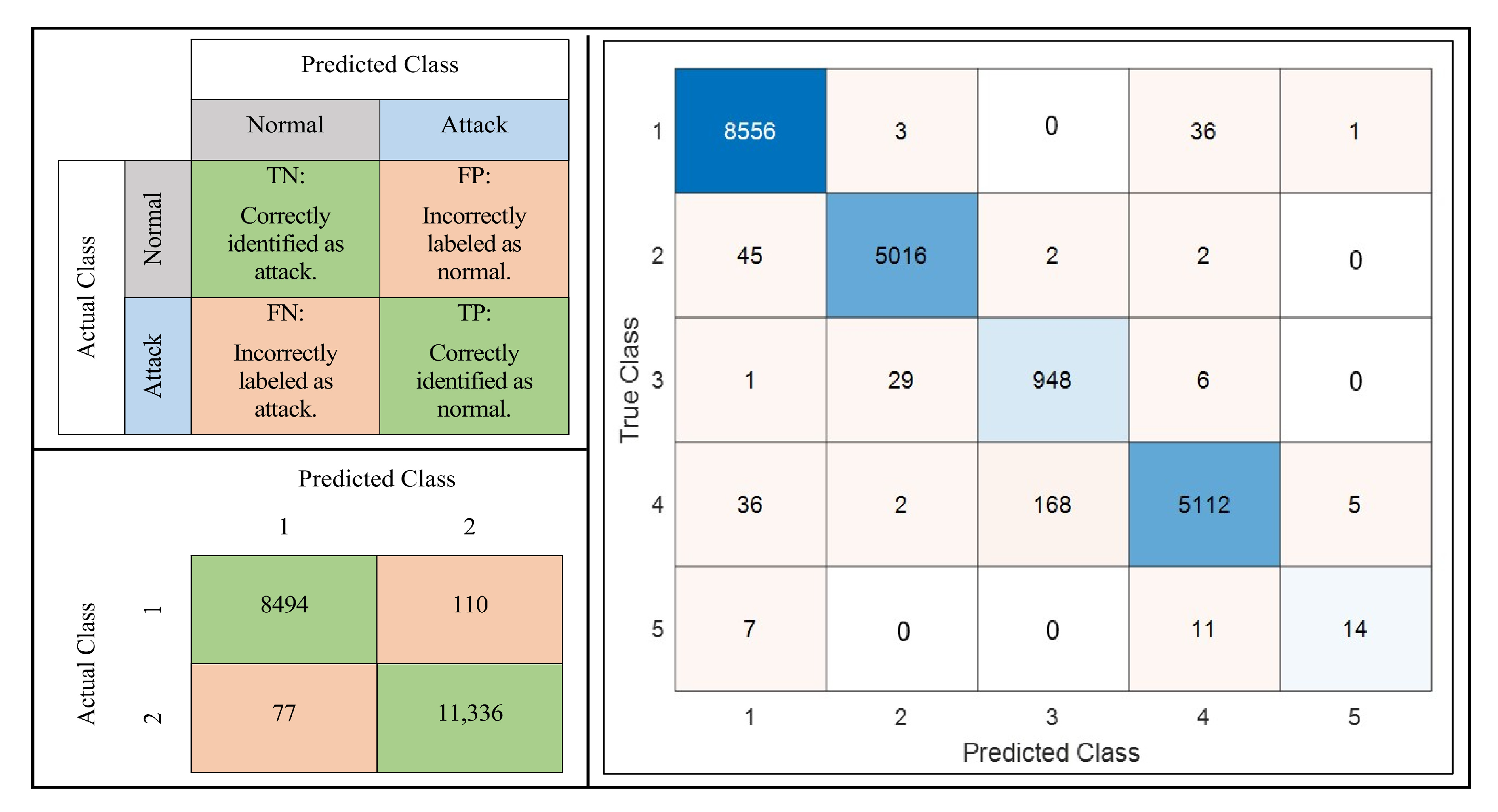
- We provide a comprehensive performance analysis to gain more insight about the system efficiency, such as the confusion matrix to analyze the attacks’ detection true/false positives and true/false negatives, along with other evaluation metrics, including precision, recall, the F-score metric, and the false alarm rate.
- We compare our findings with other related state-of-the-art works employing the same dataset, as well as with other state-of-the-art machine-learning-based intrusion detection systems (ML-IDSs) employing different datasets.
2. Dataset of Cyber-Attacks
- (a)
- It can be efficiently imported, read, preprocessed, encoded, and programmed to produce two- or multiclass classification for IoT cyber-attacks.
- (b)
- (c)
- It is obtainable as a .txt/.csv filetype consisting of a reasonable number of non-redundant records in the training and test sets. This improves the classification process by avoiding the bias toward more frequent records.
- (d)
- It correlates to high-level IoT traffic structures and cyberattacks, and it can be customized, expanded, and regenerated [29].
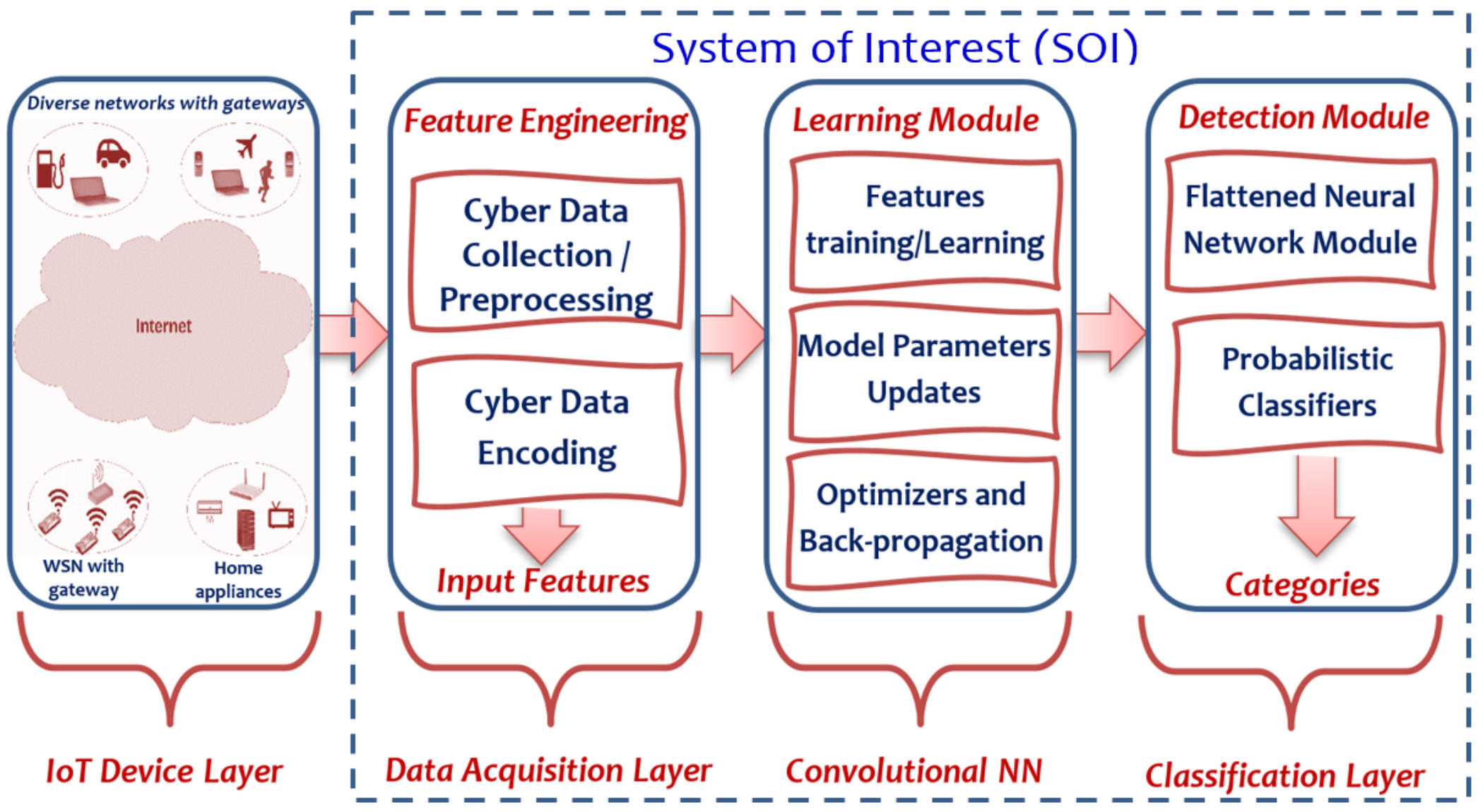
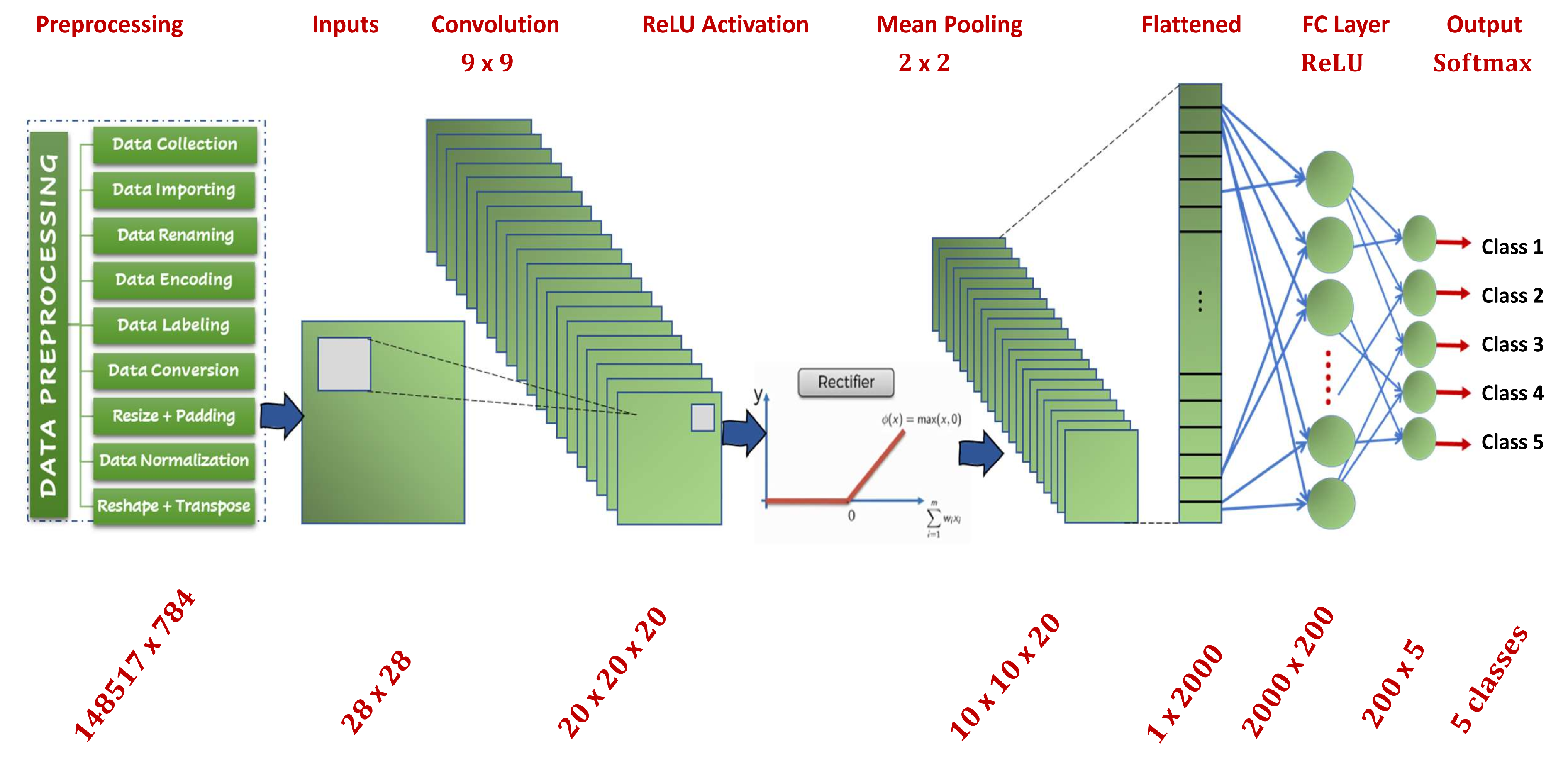
3. System Modeling
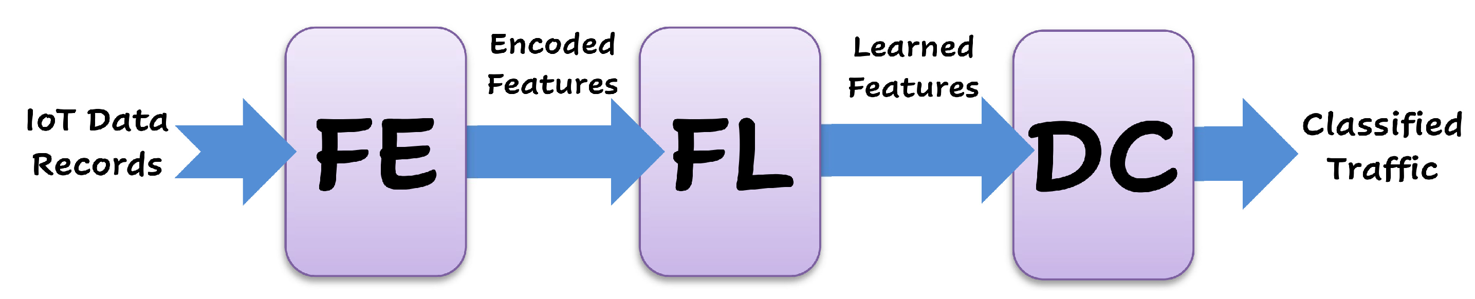
3.1. Implementation of the Feature Engineering Subsystem
- (1).
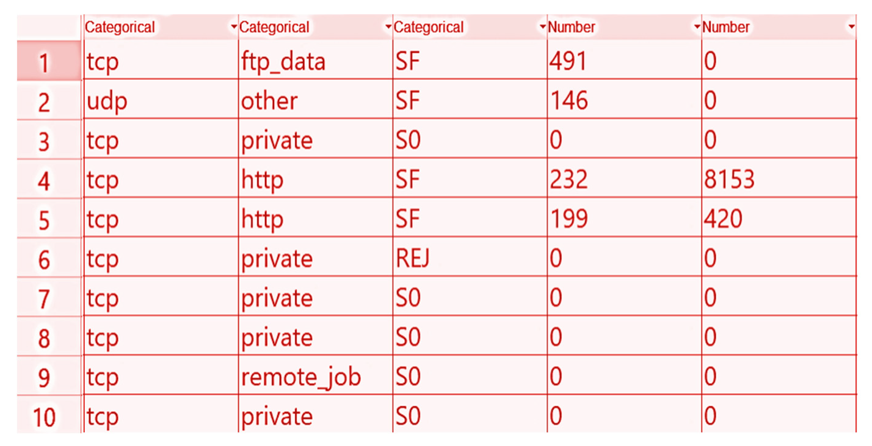
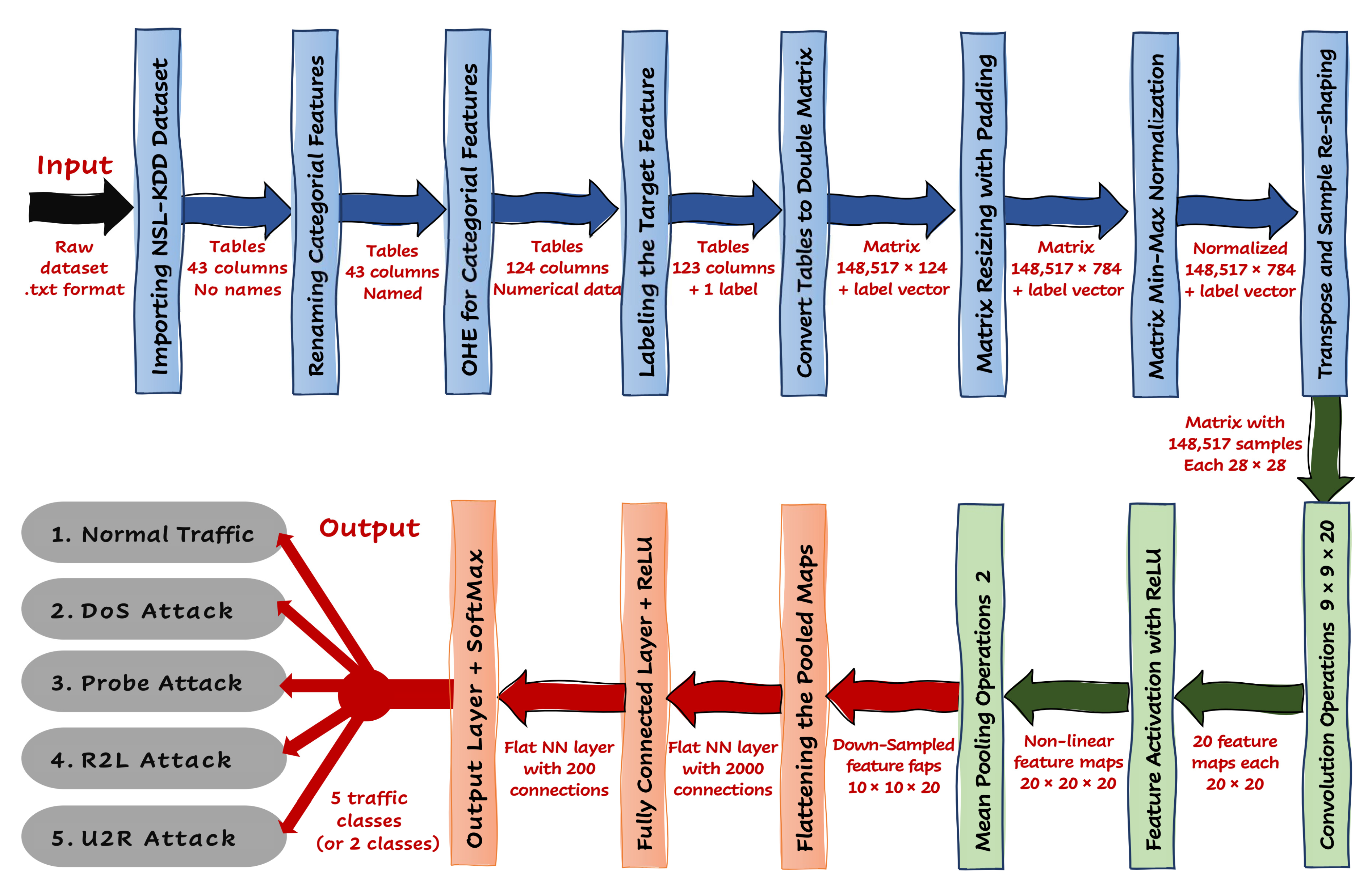
- Importing the NSL-KDD dataset: In this stage, the collected dataset was imported/read using MATLAB 2019b (by MathWorks, Inc.) in a tabulated format instead of raw data in the original dataset text files. All data columns were assigned virtual names based on the nature of the data in the cells. The imported dataset includes 43 different features/columns. Figure 4 shows a sample of an imported NSL-KDD dataset using the table datatype. The illustrated sample shows only the first ten records, along with five features. All data columns were assigned virtual names based on the nature of data in the cells.
- (2).
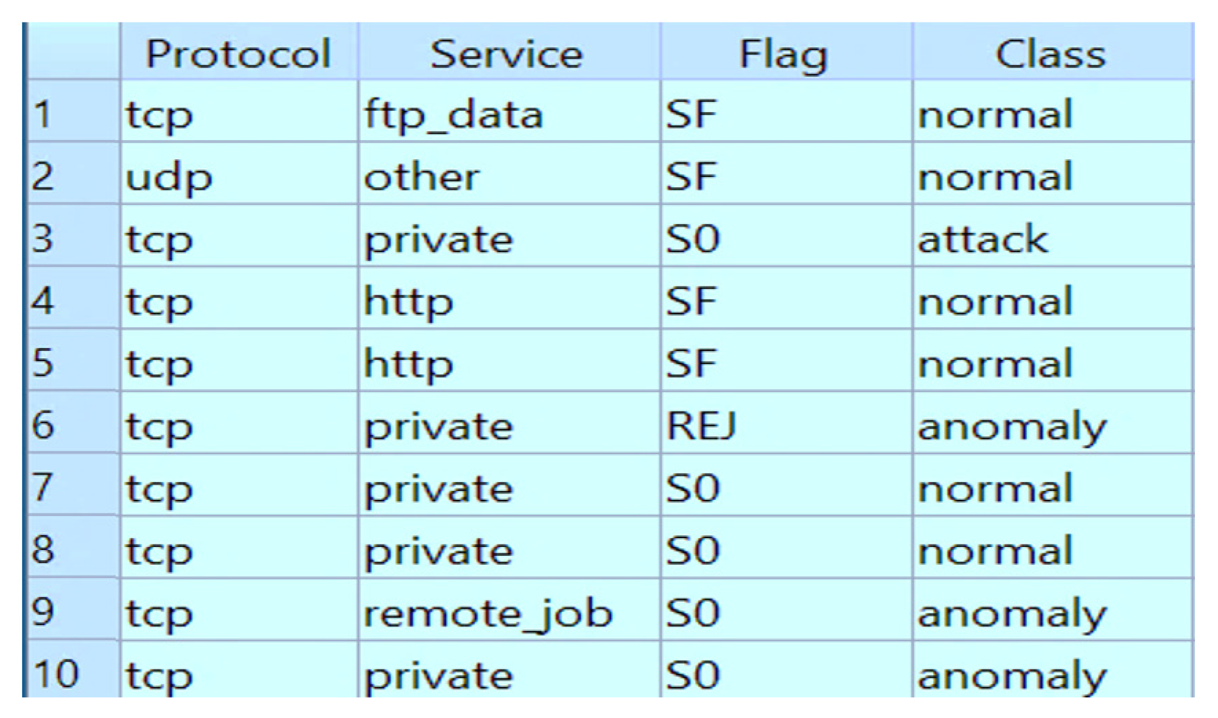
- Renaming categorical features: Four of the imported 43 features are categorical features that needed to be renamed prior to the data encoding and sample labeling processes. These features were the target protocol, the required service, the service flag, and the record category (e.g., normal or attack). Therefore, the four categorical columns were renamed accordingly in this stage. Figure 5 illustrates the four categorical features (columns) that were renamed for the binary-class data records (the other columns are omitted for better readability). Furthermore, note that the dataset encompasses multiclass data records for different traffic categories.
- (3).
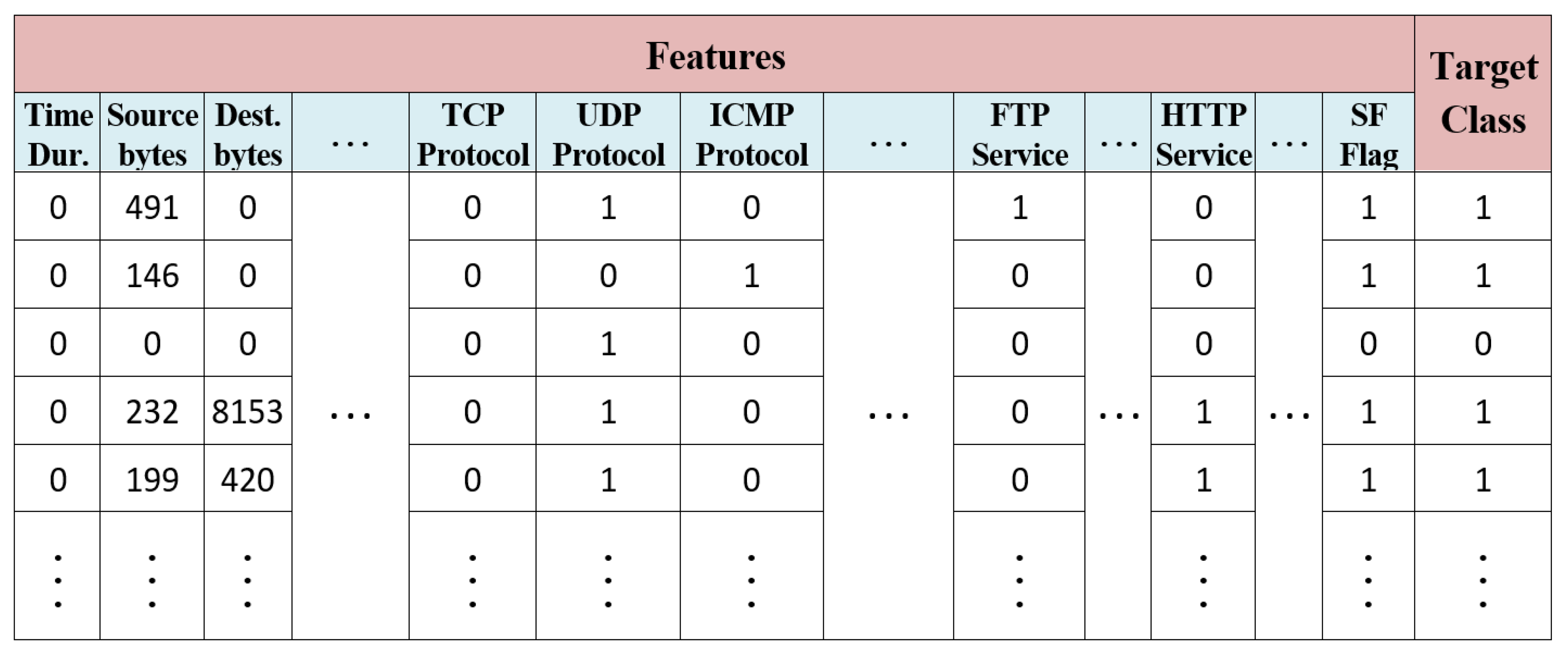
- One-hot encoding of categorical features: This module is responsible for the conversion of the categorical data records into numerical data records in order to be employed by the neural network. Therefore, three categorical features underwent a one-hot encoding process (1-N encoding) [35]. These features were the protocol column, the service column, and the flag column. The class feature/column was left for the sample-labeling process.
- For the protocol feature, three different types of protocols were revealed from the dataset, namely, TCP (Transmission Control Protocol), UDP (User Datagram Protocol), and ICMP (Internet Control Message Protocol). The one-hot encoding for this feature replaced the categorical data of the “protocol column” with the three numerical features, as shown in Table 3.
- For the service feature, 69 different services were revealed from the dataset, such as “AOL,” “AUTH,” “BGP,” “COURIER,” “CSNET_NS,” …, “UUCP_PATH,” “VMNET,” “WHOIS,” “X11,” and “Z39_50.” The one-hot encoding for this feature replaced the categorical data of the “service column” with the 69 numerical features, as shown in Table 4.
- For the flags feature, 11 different flags were revealed from the dataset, namely, “OTH,” “REJ,” “RSTO,” “RSTOS0,” “RSTR,” “S0,” “S1,” “S2,” “S3,” “SF,” and “SH.” The one-hot encoding for this feature replaced the categorical data of the “flag column” with the 11 numerical features, as shown in Table 5.
- (4).
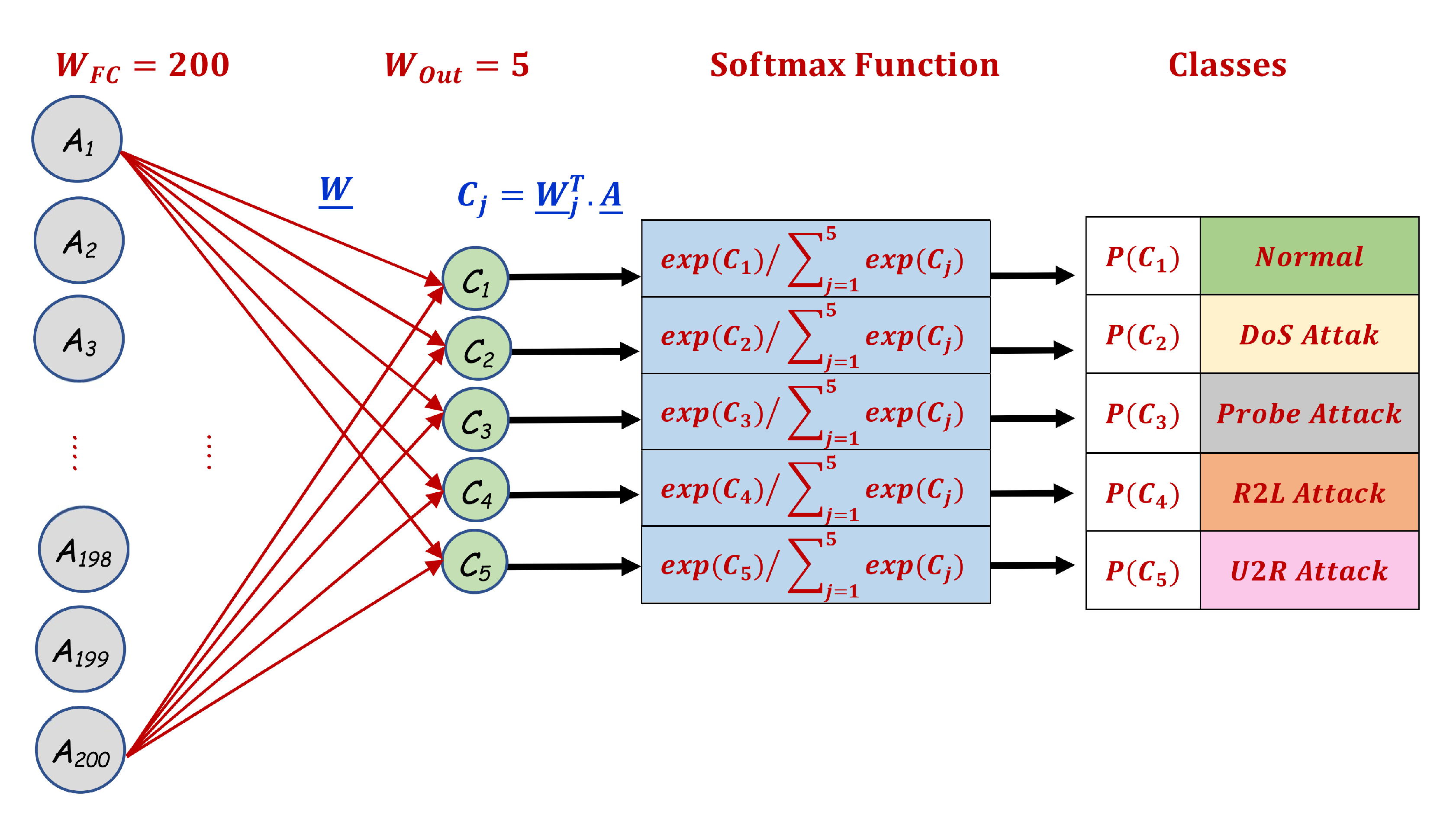
- Labeling the target feature: This stage is concerned with sample labeling using numerical (integer) labels for the target classes. Therefore, the categorical “class column” was converted to numerical classes according to the classification technique. In our system implementation, we considered two forms of traffic classifications: binary classification (1: normal vs. 2: attack) and multiple classifications (1: normal, 2: DoS, 3: probe, 4: R2L, and 5: U2R). After this stage, all data records were available in a numerical format (i.e., no categorical data existed anymore). As a result of 1-N encoding and numerical labeling, we converted the dataset into 123 features and one data label. The results of this stage, i.e., the encoded form of the dataset table of the two-class records, is provided in Figure 6.
- (5).
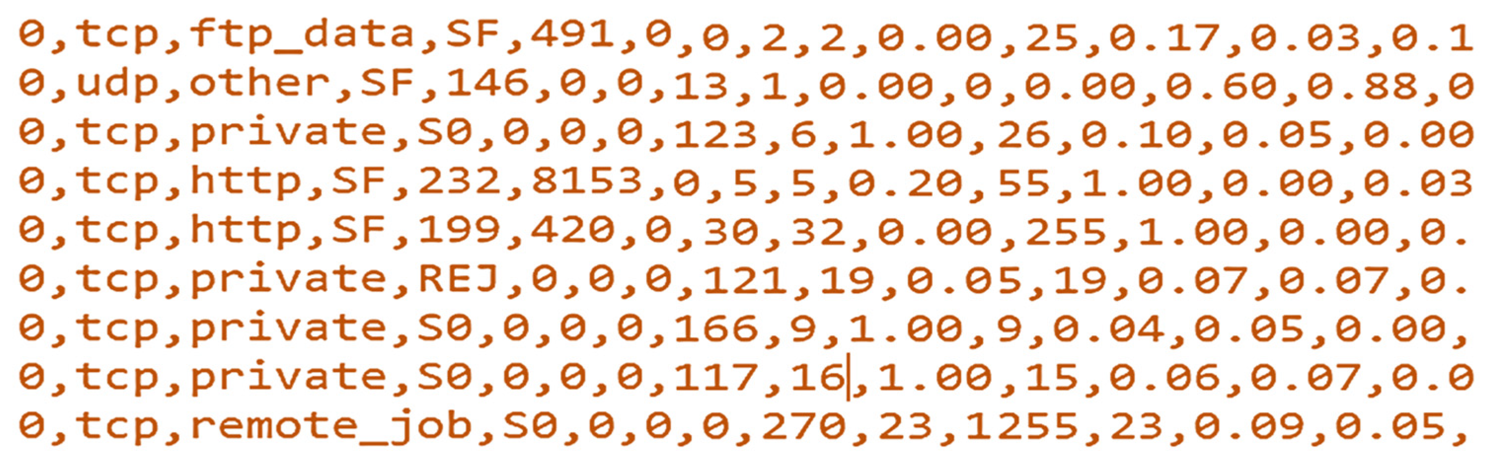
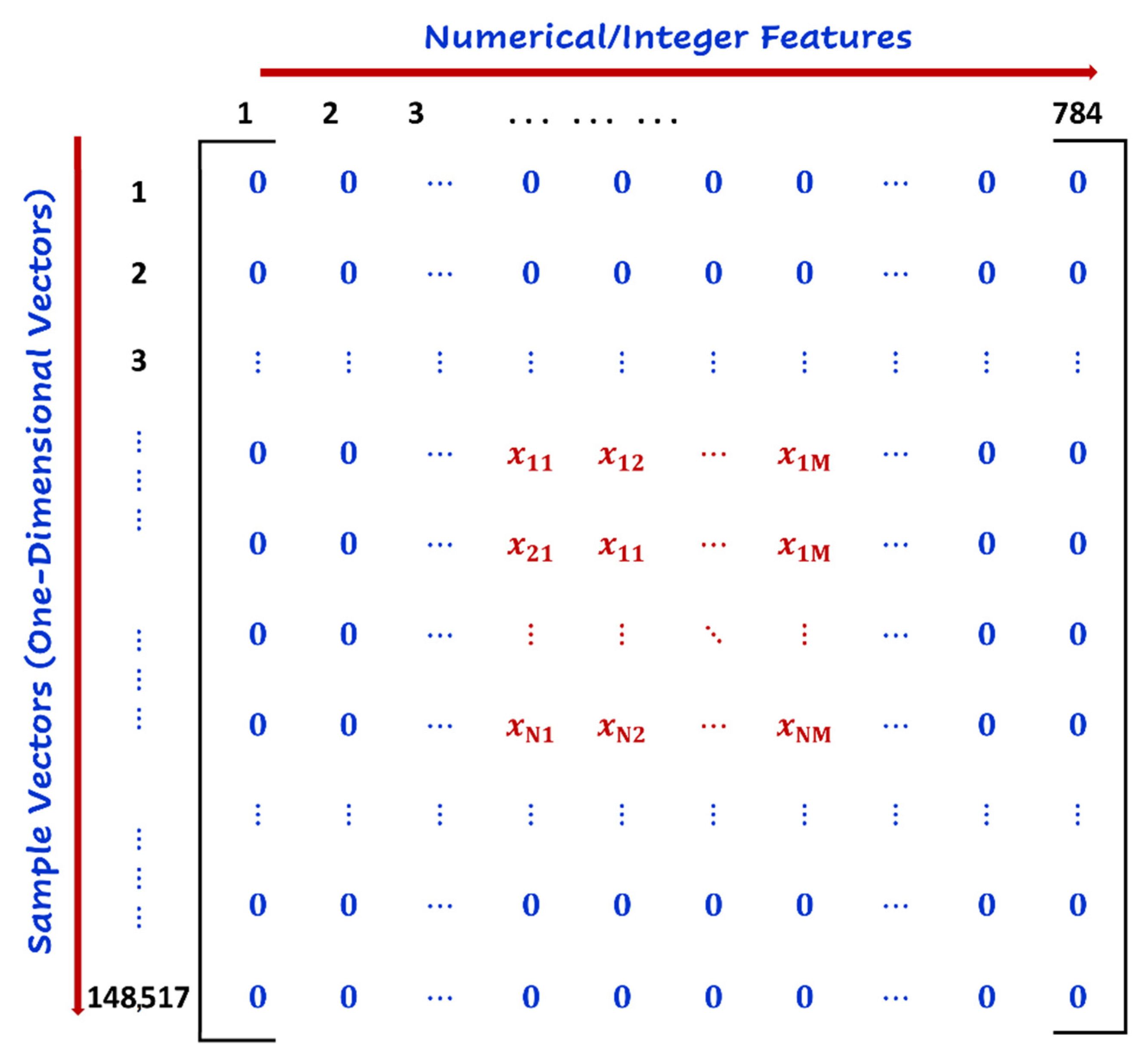
- Converting tables to a double matrix: At the end of dataset importing, encoding, and labeling processes, the dataset samples and targets should be provided to the neural network inputs of FL subsystem as a matrix of all input numerical samples. Therefore, the encoded dataset tables were converted to a double matrix (148,517 × 124). For instance, the following double matrix illustrates the first five rows of the dataset matrix.
- (6).
- Matrix resizing with a padding operation: This module is responsible for adjusting the size of the dataset matrix to accommodate the input size for the FL subsystem. This was performed by resizing the matrix of the engineered dataset from 148,517 × 124 to the new size of 148,517 × 784 since the input size of every individual sample processed at the FL subsystem was 28 × 28 = 784. Thereafter, the new empty records of this matrix were padded with a zero-padding technique [36]. To avoid any feature biasing the samples of the dataset, the padded records were distributed equally around the data samples. Figure 7 illustrates an example of resizing with the zero-padding operation used in this research. The new matrix size was composed of 148,517 sample attacks, each with 784 features.
- (7).
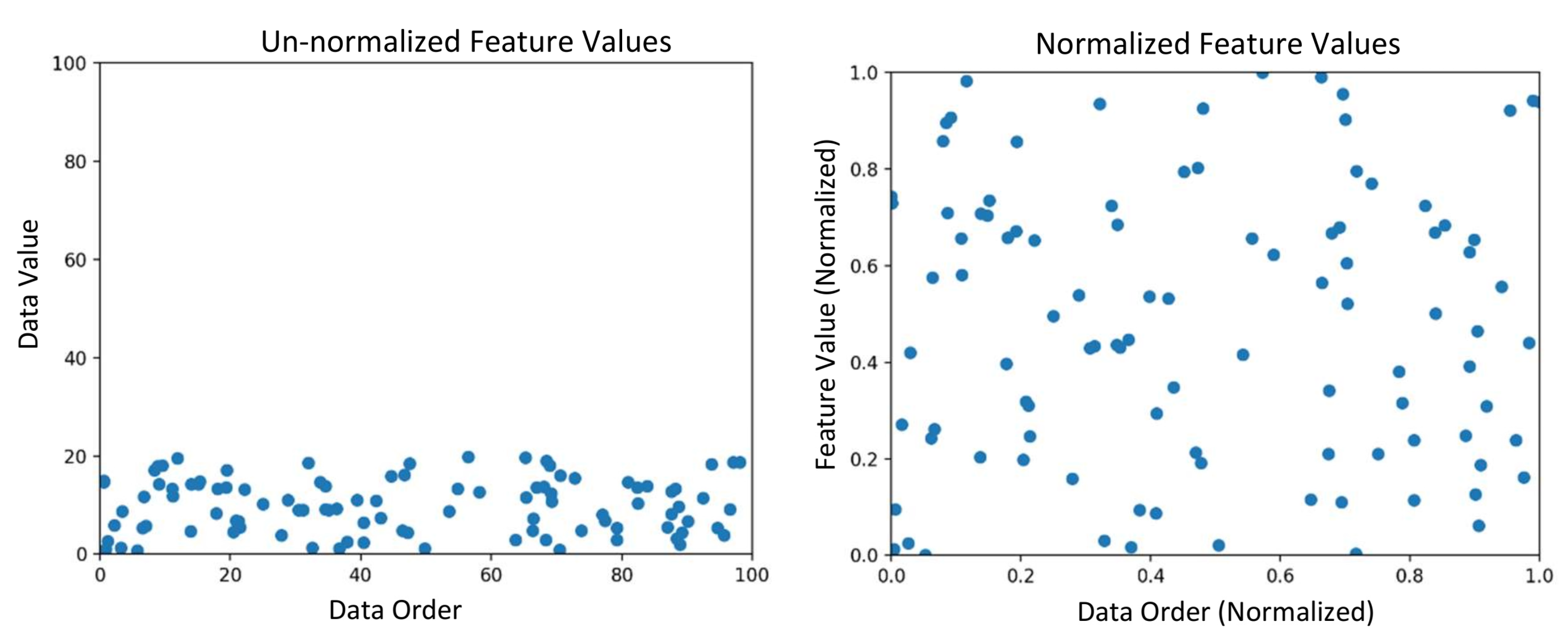
- Matrix normalization with a min-max norm: Data normalization is performed such that all the data points are in the same range (scale) with equal significance for each of them. Otherwise, one of the great value features might completely dominate the others in the dataset. Thus, this module is responsible for normalizing all integer numbers of the dataset matrix into a range between 0 and 1 using min-max normalization (MX-Norm) [37]. MX-Norm is a well-known method for normalizing data, as it is commonly used in machine learning applications. In this method, we scanned all the values in every feature, and then, the minimum value was converted into a 0 and the maximum value was converted into a 1, while the other values were converted (normalized) into a fractional value from 0 to 1. The min-max normalization for data record at the ith position of matrix X is defined as follows:Furthermore, Figure 8 illustrates an example of the integer data features normalized using min-max normalization (0–1). The effect of normalization can be clearly seen as it ensured all features were at the same scale.
- (8).
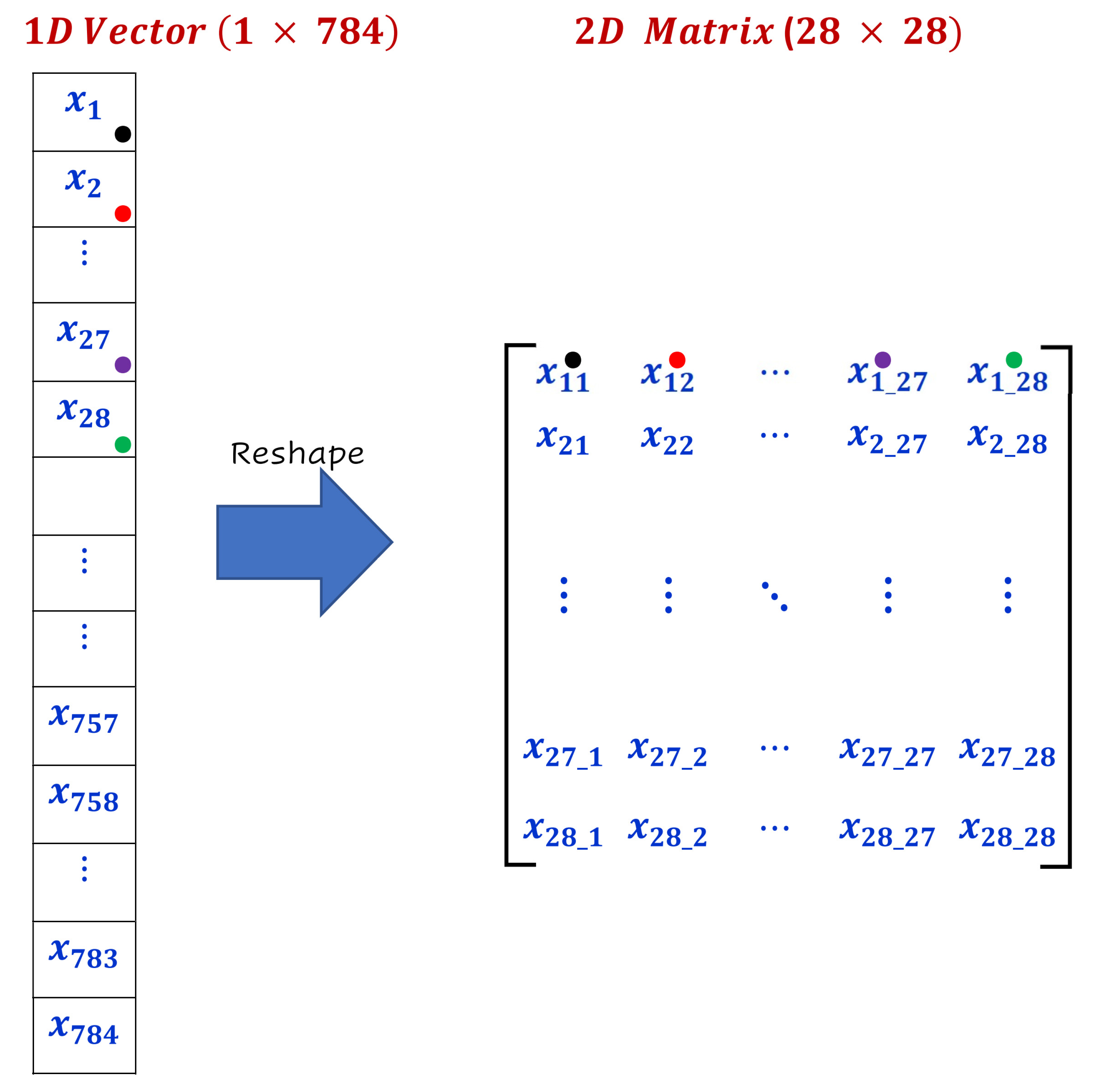
- Reshaping the double matrix: This module is responsible for creating the attack samples for the CovNet by reshaping the one-dimensional vectors of the attack records into two-dimensional square matrices to accommodate the input size for the developed CovNet network. Accordingly, every one-dimensional vector sample (1 × 784) was reshaped into a two-dimensional matrix (28 × 28) using a raw-by-raw reshaping fashion. This operation generated a square matrix for each data sample, as illustrated in Figure 9.
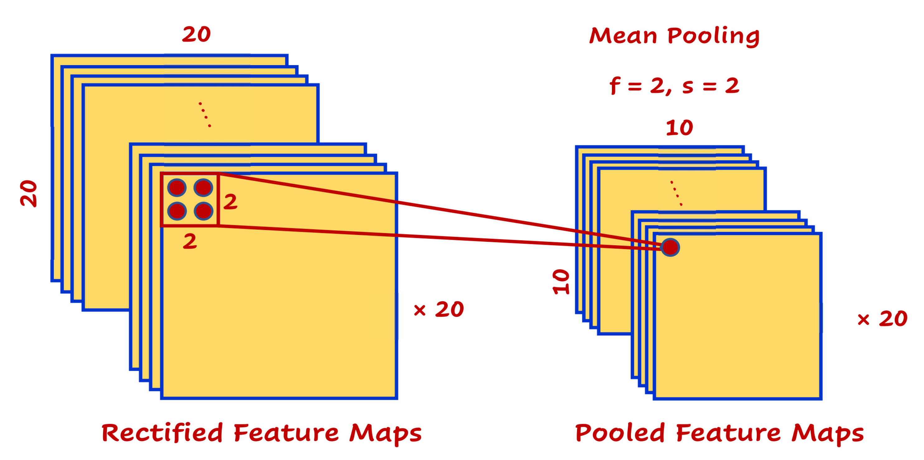
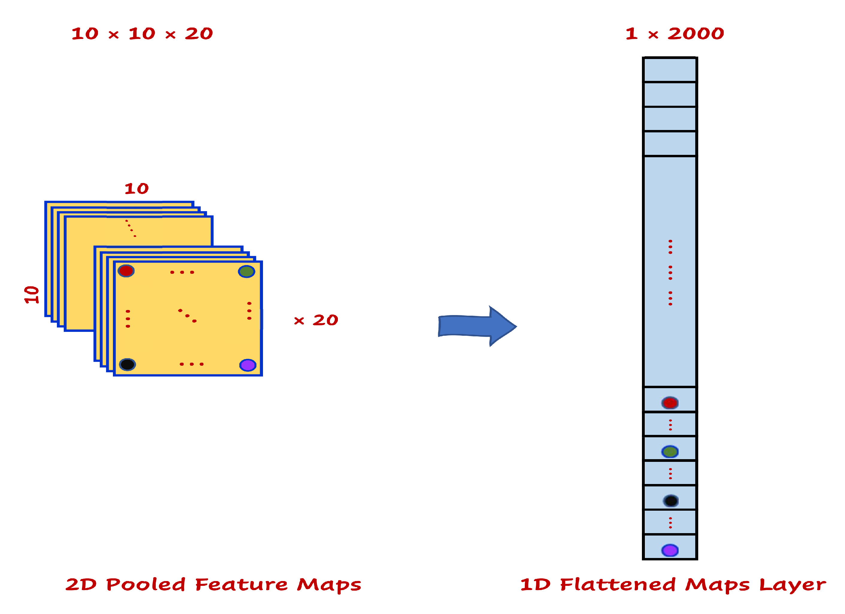
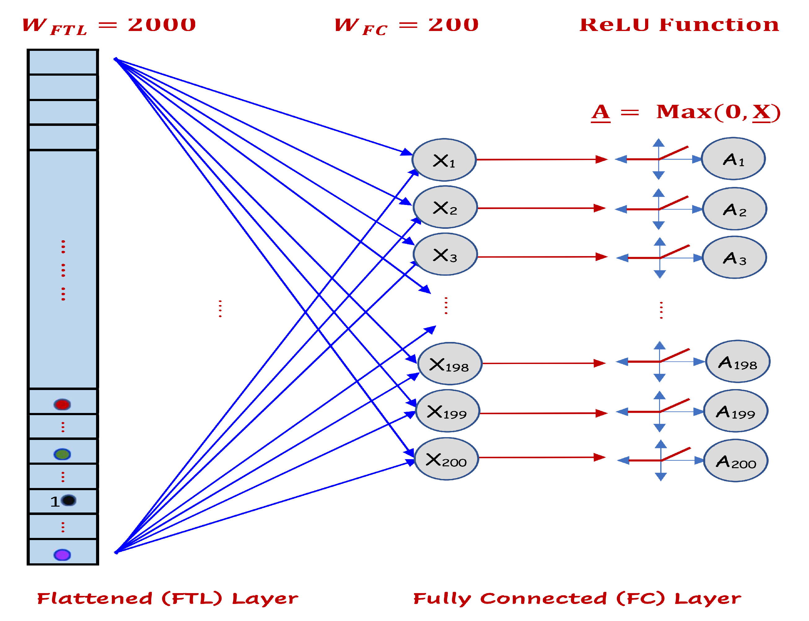
3.2. Implementation of Feature Learning Subsystem
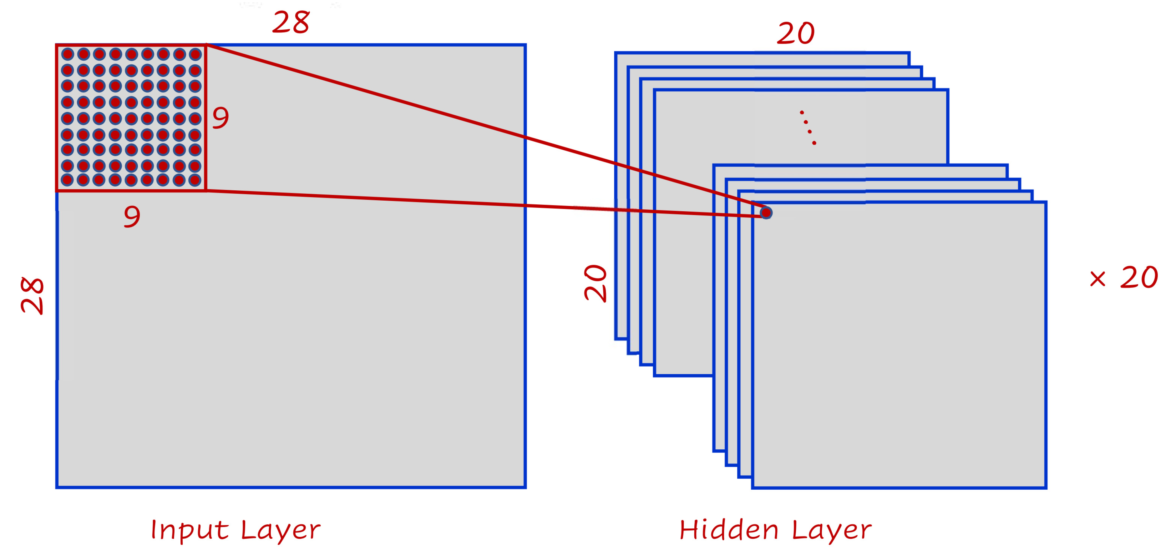
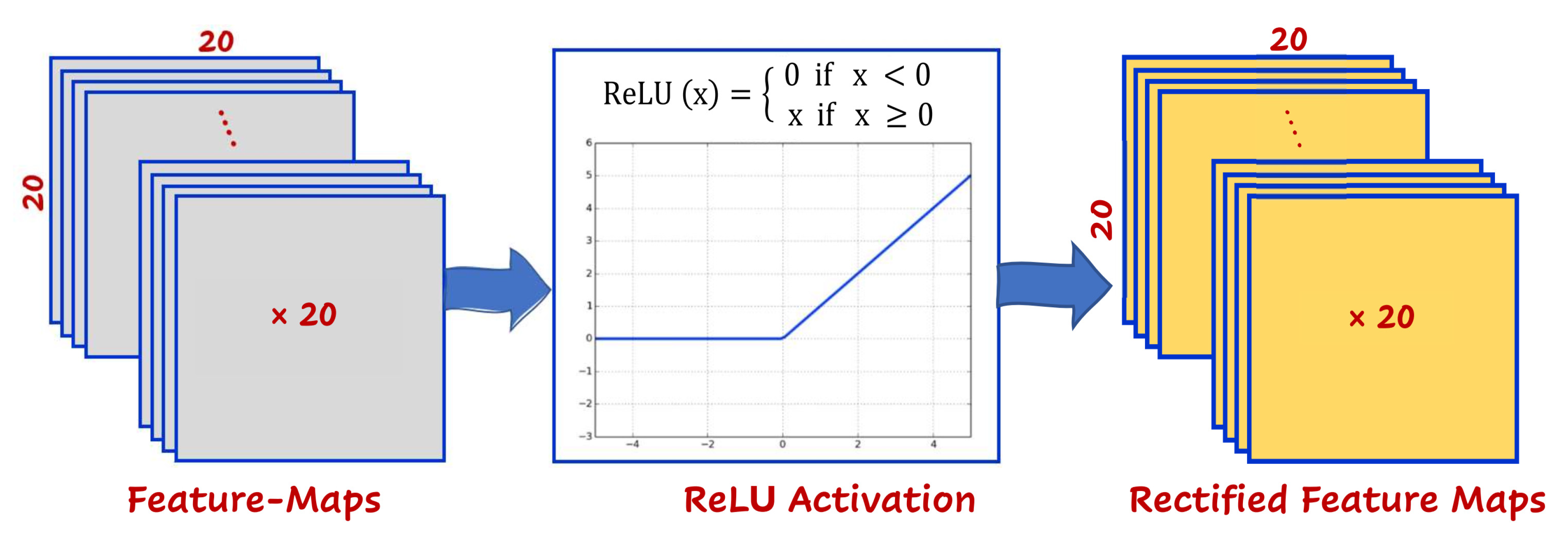
3.3. Implementation of Detection and Classification Subsystem
3.4. System Integration
4. Simulation Environment
- Dataset Distribution:
- ―
- 85% of the dataset was used for training (i.e., ≈128,500 data sample records).
- ―
- 15% of the dataset was used for testing (i.e., ≈20,000 data sample records).
- CovNet Configurations:
|
|
|
|
|
|
|
|
- Model Optimization Configurations:
- ―
- Optimization algorithm = mini batch gradient descent (find minimum loss).
- ―
- , momentum factor () = 0.95, learning rate () = 0.05.
- ―
- Momentum updates = , , .
- ―
- All momentum updates were initialized using zeros matrices ().
- Training Model Configurations:
|
|
|
|
- Weight Update Policy:
| |
|
|
|
|
|
|
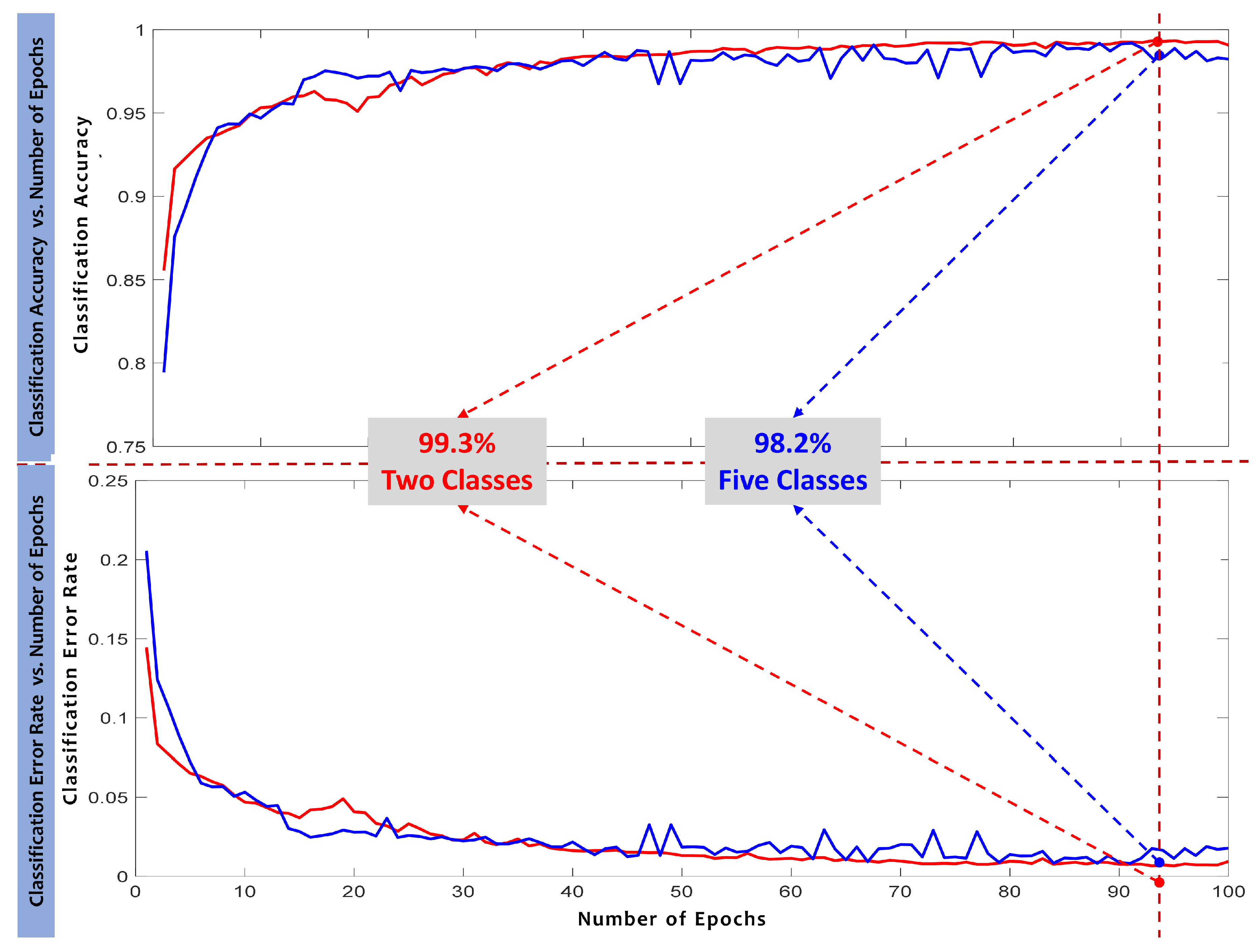
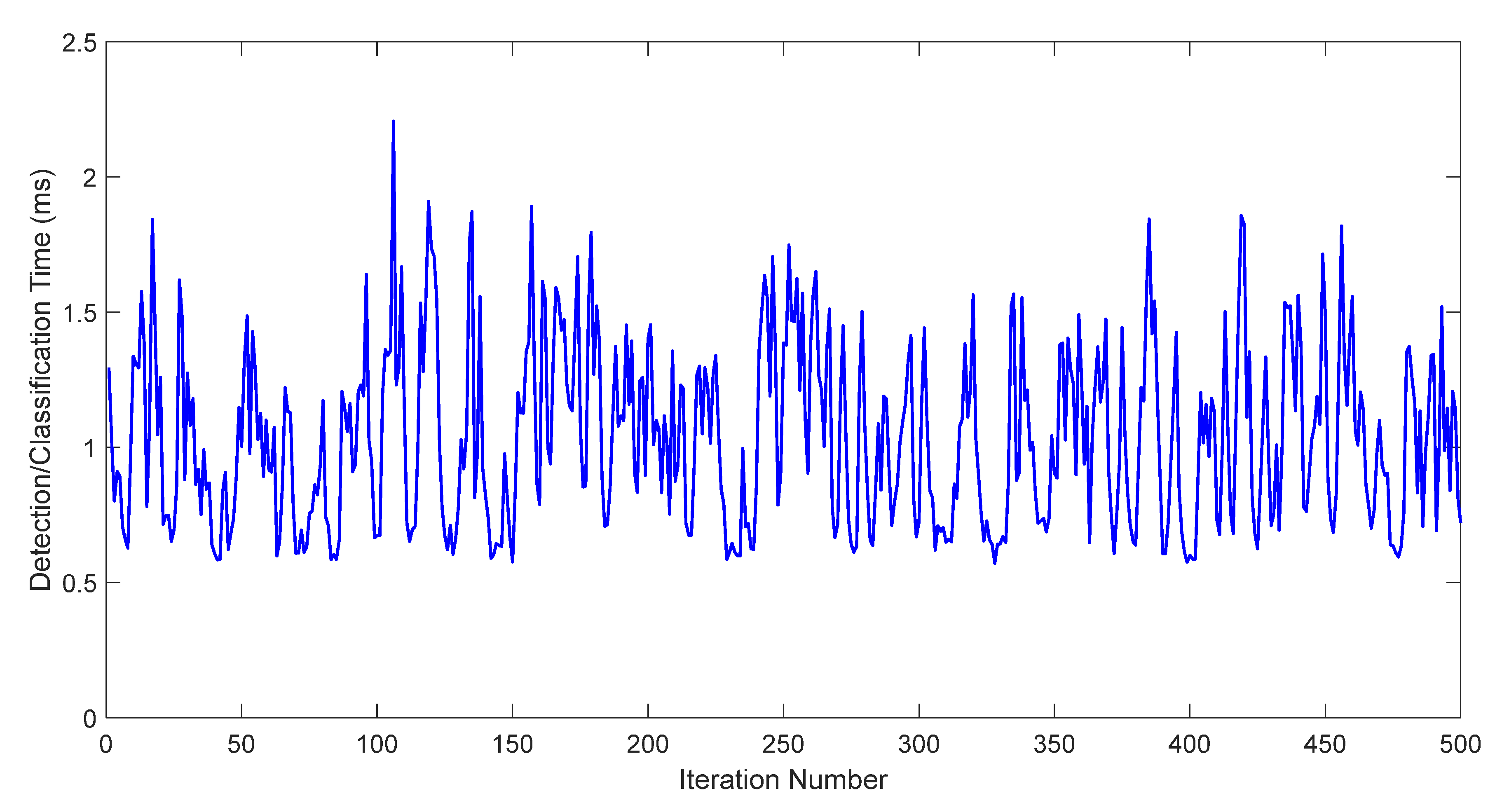
5. Results and Discussion
5.1. System Evaluation and Verification
5.2. System Validation and Benchmarking
6. Conclusions and Future Directions
- (a)
- Additional data collection by setting up a real-time IoT communication network with a sufficient number of nodes and gateways to incorporate node diversity. A future researcher can develop a new software system that can catch and investigate any data packet communicated through the IoT environment (in-going and out-going) and come up with attacks to update an existing dataset or come up with a new dataset. Note that the packet collection and investigation should be performed for a sufficient amount of time to provide more insights into the type of packet (normal or anomaly) processed during IoT networking. This can provide different perceptions of the operation of the device, such as the utilization of the processing unit, the memory unit, and the communication traffic. The collected data can then be deemed as normal or an anomaly based on their behavior. For example, the normal data is related to the imitation of usual actions of local IoT devices, such as surveillance cameras. The anomaly data concerns botnet/probe actions, such as communication with command-and-control units. In the end, the data can be labeled accordingly.
- (b)
- The proposed IoT-IDCS-CNN can be customized and used for intrusion detection by incorporating other cyberattack datasets, such as the Aegean Wireless Intrusion Dataset (AWID) dataset [44], the Canadian Institute for Cybersecurity-Intrusion Detection System (CICIDS) dataset [45], the Distributed Denial of Service (DDoS) dataset [46], and the University of New South Wales-New Bot 2015 (UNSW-NB15) dataset [47]. This can be achieved by customizing the preprocessing and output layers accordingly with fine-tuning for the hidden layers, as well as the model parameters and hyperparameters to obtain the maximum classification accuracy and the lowest error rate.
- (c)
- The proposed IoT-IDCS-CNN can also be tuned and used to perform other real-life applications that require image recognition and classification, such as medical, biomedical, and handwriting recognition applications.
- (d)
- Finally, the proposed system can be employed by an IoT gateway device to provide intrusion detection services for a network of IoT devices, such as a network of Advanced RISC Machine (ARM) Cortex based nodes. More investigation on the proposed IoT-IDCS-CNN can be reported, including power consumption, memory utilization, communication, and computation complexity over low power IoT nodes with tiny system components (such as battery-operated/energy-aware devices).
Author Contributions
Funding
Acknowledgments
Conflicts of Interest
References
- Alrawais, A.; Alhothaily, A.; Hu, C.; Cheng, X. Fog Computing for the Internet of Things: Security and Privacy Issues. IEEE Internet Comput. 2017, 21, 34–42. [Google Scholar] [CrossRef]
- Chiti, F.; Fantacci, R.; Loreti, M.; Pugliese, R. Context-aware wireless mobile automatic computing and communications: Research trends & emerging applications. IEEE Wirel. Commun. 2016, 3, 86–92. [Google Scholar] [CrossRef]
- Silva, N.; Khan, M.; Han, K. Internet of Things: A Comprehensive Review of Enabling Technologies, Architecture, and Challenges. IETE Tech. Rev. 2017, 35, 1–16. [Google Scholar] [CrossRef]
- Mahmoud, R.; Yousuf, T.; Aloul, F.; Zualkernan, I. Internet of things (IoT) security: Current status, challenges, and prospective measures. In Proceedings of the 10th International Conference for Internet Technology and Secured Transactions (ICITST), London, UK, 14–16 December 2015; pp. 336–341. [Google Scholar] [CrossRef]
- Wazid, M.; Das, A.K.; BhBat, V.; Vasilakos, A.V. LAM-CIoT: Lightweight authentication mechanism in cloud-based IoT environment. J. Netw. Comput. Appl. 2020, 150. [Google Scholar] [CrossRef]
- Mollah, M.B.; Azad, M.A.K.; Vasilakos, A. Secure Data Sharing and Searching at the Edge of Cloud-Assisted Internet of Things. IEEE Cloud Comput. 2017, 4, 34–42. [Google Scholar] [CrossRef]
- Paar, J.P. Understanding Cryptography; Springer: Berlin/Heidelberg, Germany, 2010; pp. 1–87. [Google Scholar] [CrossRef]
- Caspi, G. Introducing Deep Learning: Boosting Cybersecurity with an Artificial Brain. Informa Tech, Dark Reading, Analytics. 2016. Available online: http://www.darkreading.com/analytics (accessed on 18 February 2019).
- Bendiab, G.; Shiaeles, S.; Alruban, A.; Kolokotronis, N. IoT Malware Network Traffic Classification using Visual Representation and Deep Learning. In Proceedings of the 6th IEEE Conference on Network Softwarization (NetSoft), Ghent, Belgium, 29 June–3 July 2020; pp. 444–449. [Google Scholar] [CrossRef]
- Shire, R.; Shiaeles, S.; Bendiab, K.; Ghita, B.; Kolokotronis, N. Malware Squid: A Novel IoT Malware Traffic Analysis Framework Using Convolutional Neural Network and Binary Visualization. In Proceedings of the Internet of Things, Smart Spaces, and Next Generation Networks and Systems. NEW2AN 2019, ruSMART. Lecture Notes in Computer Science; Springer: Cham, Switzerland, 2019; Volume 11660. [Google Scholar] [CrossRef] [Green Version]
- Baptista, I.; Shiaeles, S.; Kolokotronis, N. A Novel Malware Detection System Based On Machine Learning and Binary Visualization. In Proceedings of the IEEE International Conference on Communications (IEEE ICC), Shanghai, China, 20–24 May 2019; pp. 1–6. [Google Scholar]
- Taher, K.A.; Jisan, B.M.Y.; Rahman, M.M. Network Intrusion Detection using Supervised Machine Learning Technique with Feature Selection. In Proceedings of the International Conference on Robotics, Electrical and Signal Processing Techniques (ICREST), Bangladesh, South Asia, 10–12 January 2019; pp. 643–646. [Google Scholar] [CrossRef]
- Gao, X.; Shan, C.; Hu, C.; Niu, Z.; Liu, Z. An Adaptive Ensemble Machine Learning Model for Intrusion Detection. IEEE Access 2019, 7, 82512–82521. [Google Scholar] [CrossRef]
- Sapre, S.; Ahmadi, P.; Islam, K. A Robust Comparison of the KDDCup99 and NSL-KDD IoT Network Intrusion Detection Datasets through Various Machine Learning Algorithms. arXiv 2019, arXiv:1912.13204v1. [Google Scholar]
- Chowdhury, M.M.U.; Hammond, F.; Konowicz, G.; Xin, C.; Wu, H.; Li, J. A few-shot deep learning approach for improved intrusion detection. In Proceedings of the 2017 IEEE 8th Annual Ubiquitous Computing, Electronics and Mobile Communication Conference (UEMCON), New York, NY, USA, 19–21 October 2017; pp. 456–462. [Google Scholar] [CrossRef]
- Javaid, A.; Niyaz, Q.; Sun, W.; Alam, M. A Deep Learning Approach for Network Intrusion Detection System. In Proceedings of the 9th EAI International Conference on Bio-inspired Information and Communications Technologies (formerly BIONETICS), New York, NY, USA, 24 May 2016; pp. 21–26. [Google Scholar] [CrossRef] [Green Version]
- Imamverdiyev, Y.; Sukhostat, L. Anomaly detection in network traffic using extreme learning machine. In Proceedings of the 2016 IEEE 10th International Conference on Application of Information and Communication Technologies (AICT), Baku, Azerbaijan, 12–14 October 2016; pp. 1–4. [Google Scholar] [CrossRef]
- Jan, S.U.; Ahmed, S.; Shakhov, V.; Koo, I. Toward a Lightweight Intrusion Detection System for the Internet of Things. IEEE Access 2019, 7, 42450–42471. [Google Scholar] [CrossRef]
- Roopak, M.; Tian, G.Y.; Chambers, J. Deep Learning Models for Cyber Security in IoT Networks. In Proceedings of the 2019 IEEE 9th Annual Computing and Communication Workshop and Conference (CCWC), Las Vegas, NV, USA, 7–9 January 2019; pp. 0452–0457. [Google Scholar] [CrossRef]
- Ioannou, C.; Vassiliou, V. Classifying Security Attacks in IoT Networks Using Supervised Learning. In Proceedings of the 2019 15th International Conference on Distributed Computing in Sensor Systems (DCOSS), Santorini Island, Greece, 29–31 May 2019; pp. 652–658. [Google Scholar] [CrossRef]
- Brun, O.; Yin, Y.; Gelenbe, E. Deep Learning with Dense Random Neural Network for Detecting Attacks against IoT-connected Home Environments. Procedia Comput. Sci. 2018, 134, 458–463. [Google Scholar] [CrossRef]
- Thing, V.L.L. IEEE 802.11 Network Anomaly Detection and Attack Classification: A Deep Learning Approach. In Proceedings of the 2017 IEEE Wireless Communications and Networking Conference (WCNC), San Francisco, CA, USA, 19–22 March 2017; pp. 1–6. [Google Scholar] [CrossRef]
- Shukla, P. ML-IDS: A machine learning approach to detect wormhole attacks in Internet of Things. In Proceedings of the 2017 Intelligent Systems Conference (IntelliSys), London, UK, 7–8 September 2017; pp. 234–240. [Google Scholar] [CrossRef]
- Hodo, E.; Bellekens, X.; Hamilton, A.; Dubouilh, P.-L.; Iorkyase, E.; Tachtatzis, C.; Atkinson, R. Threat analysis of IoT networks using artificial neural network intrusion detection system. In Proceedings of the 2016 International Symposium on Networks, Computers and Communications (ISNCC), Yasmine Hammamet, Tunisia, 11–13 May 2016; pp. 1–6. [Google Scholar] [CrossRef] [Green Version]
- Kolias, C.; Kambourakis, G.; Stavrou, A.; Gritzalis, S. Intrusion Detection in 802.11 Networks: Empirical Evaluation of Threats and a Public Dataset. IEEE Commun. Surv. Tutor. 2016, 18, 184–208. [Google Scholar] [CrossRef]
- Jang, S.-B.; Li, Y.; Ma, R.; Jiao, R. Collaborative Documentation Process Model. Int. J. Softw. Eng. Its Appl. 2015, 9, 219–232. [Google Scholar] [CrossRef]
- Ozgur, A.; Erdem, H. A review of KDD99 dataset usage in intrusion detection and machine learning between 2010 and 2015. PEERJ Prepr. 2016, 4, e1954v1. [Google Scholar] [CrossRef] [Green Version]
- Stolfo, S.; Fan, W.; Lee, W.; Prodromidis, A.; Chan, P. Cost-based modeling for fraud and intrusion detection: Results from the JAM project. In Proceedings of the DARPA Information Survivability Conference and Exposition. DISCEX’00, Hilton Head, SC, USA, 25–27 January 2000; Volume 2, pp. 130–144. [Google Scholar] [CrossRef] [Green Version]
- Revathi, S.; Malathi, A. A Detailed Analysis on NSL-KDD Dataset Using Various Machine Learning Techniques for Intrusion Detection. Int. J. Eng. Res. Technol. (IJERT) 2013, 2, 1848–1853. [Google Scholar]
- Canadian Institute for Cybersecurity (CIS). NSL-KDD Dataset. Available online: https://www.unb.ca/cic/datasets/nsl.html (accessed on 10 April 2019).
- Kolias, C.; Kambourakis, G.; Stavrou, A.; Voas, J. DDoS in the IoT: Mirai and Other Botnets. J. Computers 2017, 50, 80–84. [Google Scholar] [CrossRef]
- Ambedkar, C.; Babu, V.K. Detection of Probe Attacks Using Machine Learning Techniques. Int. J. Res. Stud. Comput. Sci. Eng. (IJRSCSE) 2015, 2, 25–29. [Google Scholar]
- Pongle, P.; Chavan, G. A survey: Attacks on RPL and 6LoWPAN in IoT. In Proceedings of the 2015 International Conference on Pervasive Computing (ICPC), Pune, India, 8–10 January 2015; pp. 1–6. [Google Scholar] [CrossRef]
- Bengio, Y.; Courville, A.; Vincent, P. Representation Learning: A Review and New Perspectives. IEEE Trans. Pattern Anal. Mach. Intell. 2013, 35, 1798–1828. [Google Scholar] [CrossRef]
- Sarkar, D.J. Understanding Feature Engineering. Towards Data Science. Medium. 2018. Available online: https://towardsdatascience.com/tagged/tds-feature-engineering (accessed on 2 January 2019).
- Brownlee, J. A Gentle Introduction to Padding and Stride for Convolutional Neural Networks. Deep Learning for Computer Vision, Machine Learning Mastery. 2019. Available online: https://machinelearningmastery.com/padding-and-stride-for-convolutional-neural-networks (accessed on 8 March 2019).
- Kalay, A.F. Preprocessing for Neural Networks—Normalization Techniques. Machine Learning, Github.IO. Available online: https://alfurka.github.io/2018-11-10-preprocessing-for-nn.2018 (accessed on 14 May 2019).
- Li, F. CS231n: Convolutional Neural Networks for Visual Recognition. Computer Science, Stanford University. 2019. Available online: http://cs231n.stanford.edu (accessed on 15 March 2019).
- Brownlee, J. A Gentle Introduction to the Rectified Linear Unit (ReLU). Deep Learning for Computer Vision, Machine Learning Master. 2019. Available online: https://machinelearningmastery.com (accessed on 14 May 2019).
- INCOSE. INCOSE Systems Engineering Handbook, version 3.2.2; INCOSE-TP-2003-002-03.2.2; International Council on Systems Engineering (INCOSE): San Diego, CA, USA, 2012. [Google Scholar]
- Narkhede, S. Understanding Confusion Matrix. Medium: Towards data science. 2018. Available online: https://towardsdatascience.com/understanding-confusion-matrix-a9ad42dcfd62 (accessed on 12 January 2020).
- Kim, P. MATLAB Deep Learning with Machine Learning, Neural Networks and Artificial Intelligence. Apress: Part of Springer Nature. 2017. Available online: https://www.apress.com/gp/book/9781484228449 (accessed on 10 October 2020).
- Gupta, P. Cross-Validation in Machine Learning. Medium: Towards data science. 2017. Available online: https://towardsdatascience.com/cross-validation-in-machine-learning-72924a69872f (accessed on 13 February 2020).
- Kolias, C.; Kambourakis, G.; Gritzalis, S. Attacks and countermeasures on 802.16: Analysis & assessment. IEEE Commun. Surv. Tuts 2013, 15, 487–514. [Google Scholar] [CrossRef] [Green Version]
- CICIDS Dataset. DS-0917: Intrusion Detection Evaluation Dataset. Available online: https://www.impactcybertrust.org/dataset_view?idDataset=917 (accessed on 2 February 2020).
- DDoS Dataset. Distributed Denial of Service (DDoS) attack Evaluation Dataset. Available online: https://www.unb.ca/cic/datasets/ddos-2019.html (accessed on 2 February 2020).
- Moustafa, N.; Slay, J. UNSW-NB15: A comprehensive data set for network intrusion detection systems (UNSW-NB15 network data set). In Proceedings of the 2015 Military Communications and Information Systems Conference (MilCIS), Canberra, ACT, Australia, 10–12 November 2015; pp. 1–6. [Google Scholar] [CrossRef]


| Research | Method | Description |
|---|---|---|
| G. Bendiab et al. 2020 [9] | Residual neural network (ResNet-50) | Two classes, utilized transfer learning with a 50-layer CovNet, employed pcap files containing pre-captured network traffic (normal/abnormal). |
| R. Shire et al. 2019 [10] | Convolutional neural network (CNN) | Five classes, employed CNN (single convolution layer + multilayer NN), three subsystems (sniffer-based traffic collection, American Standard Code For Information Interchange (ASCII)-based 2D traffic visualization, TensorFlow NN traffic analysis). |
| I. Baptista et al. 2019 [11] | Self-organizing incremental neural network (SOINN) | Five classes of malware with five filetypes, color-based binary visualization of ASCII for pre-captured files (.exe, .doc, .pdf, .txt, .htm). |
| K. Taher et al. 2019 [12] | Artificial neural network (ANN) with a support vector machine (SVM) classifier | Three classes, with 2 hidden layers and used only 35 features. |
| X. Gao et al. 2019 [13] | Deep neural network (DNN) with ensemble voting | Five classes with three methods: decision tree, random forest, K-nearest. |
| S. Sapre et al. 2019 [14] | Different machine-learning-based intrusion detection system (ML-IDS) techniques | Five classes, with two hidden layers and a naïve Bayes classifier. |
| S. Jan et al. 2019 [18] | ML-IDS-based SVM system | Only binary classification, used only two or three simple features. |
| M. Roopak et al. 2019 [19] | Deep neural network (DNN) | Small representative sample, did not reflect a realistic accuracy in actual IoT environments. |
| C. Ioannou et al. 2019 [20] | ML-IDS-based SVM system | Only used a binary classification, used an anonymous sensor topology. |
| O. Brun et al., 2018 [21] | Deep neural network (DNN) | System validation was poorly accomplished on a testbed comprising only three devices and naïve attacks were used to validate the system using real-time data with 50,000 samples. |
| V. Thing et al. 2017 [22] | Deep auto-encoder (DAE) | Unrealistic, very small dataset (no Distributed Denial of Service (DDoS), no probe), three hidden layers (256/128/64), needed significant time for feature engineering (FE). |
| P. Shukla et al. 2017 [23] | Neural network hybrid learning (K means plus decision trees) | Only used a binary classification, small-scale simulated network (16 nodes) with different topologies. |
| E, Hodo et al. 2016 [24] | Multi-layer perceptron (MLP) neural network | Unrealistic, small dataset with binary classes. |
| C. Kolias et al. 2016 [25] | Different ML-IDS techniques | Very time-consuming manual feature selection with four classes. |
| Y. Li et al. 2015 [26] | Hybrid NN (autoencoder + deep belief NN) | Redundant dataset needs to be up to date to reflect more rational results. |
| Data Groups | Two-Class Dataset | Multiclass Dataset | |||||
|---|---|---|---|---|---|---|---|
| Normal | Attack | Normal | DoS | Probe | R2L | U2R | |
| Training | 67,343 | 58,630 | 67,343 | 45,927 | 11,656 | 995 | 52 |
| Testing | 9711 | 12,833 | 9711 | 7458 | 2754 | 2421 | 200 |
| Total | 77,054 | 71,463 | 77,054 | 53,385 | 14,410 | 3416 | 252 |
| Protocol | Equivalent One-Hot Encoding | ||
|---|---|---|---|
| TCP_Protocol | UDP_Protocol | ICMP_Protocol | |
| TCP | 1 | 0 | 0 |
| UDP | 0 | 1 | 0 |
| ICMP | 0 | 0 | 1 |
| Service | Equivalent One-Hot Encoding | ||||
|---|---|---|---|---|---|
| AOL _Service | AUTH_Service | BGP_Service | . . . | Z39_50_Service | |
| AOL | 1 | 0 | 0 | . . . | 0 |
| AUTH | 0 | 1 | 0 | . . . | 0 |
| BGP | 0 | 0 | 1 | . . . | 0 |
| . | . | . | . | . | |
| . | . | . | . | . | |
| . | . | . | . | . | |
| Z39_50 | 0 | 0 | 0 | . . . | 1 |
| Flag | Equivalent One-Hot Encoding | ||||
|---|---|---|---|---|---|
| OTH_Flag | REJ_Flag | RSTO_Flag | . . . | SF_Flag | |
| “OTH” | 1 | 0 | 0 | . . . | 0 |
| “REJ” | 0 | 1 | 0 | . . . | 0 |
| “RSTO” | 0 | 0 | 1 | . . . | 0 |
| . | . | . | . | . | |
| . | . | . | . | . | |
| . | . | . | . | . | |
| “SH” | 0 | 0 | 0 | . . . | 1 |
| Item | Multiclass Dataset | ||||
|---|---|---|---|---|---|
| Normal | DoS | Probe | R2L | U2R | |
| Label | 1 | 2 | 3 | 4 | 5 |
| Probability | 0.001 | 0.040 | 0.008 | 0.950 | 0.001 |
| Layer | Comment | Trainable Parameters |
|---|---|---|
| Preprocessing | 148,517 samples each (28 × 28) | - |
| Input | 28 × 28 nodes (784 nodes) | - |
| Convolution | 20 convolution filters (9 × 9) + ReLU | WCon (9 × 9 × 20) |
| Pooling | Mean pooling (2 × 2) | - |
| Flattening | 2000 nodes | - |
| Fully connected | 200 nodes + ReLU | WFCL (2000 × 200) |
| Output | 5 nodes (or 2 nodes) + softmax | WOut (200 × 5) |
| System Unit | Specifications |
|---|---|
| Processor Unit (CPU) | Intel Core I9-9900 CPU, 8 cores, @4900 MHz |
| Graphics Card (GPU) | NVIDIA Quad P2000@1480 MHz, 5 GB memory, 1024 CUDA cores |
| Cache Memory ($) | 16 MB cache @ 3192 MHz |
| Main Memory (RAM) | 32 GB DDR4 @ 2666 MHz |
| Operating System (OS) | 64 bit, Windows 10 Pro |
| Hard Disk Drive (HD) | SATA 1TB drive + 256 GB SSD |
| Evaluation Metrics | Two-Class Classification | Five-Class Classification |
|---|---|---|
| Correctly predicted samples | 19860 | 19640 |
| Incorrectly predicted samples | 140 | 360 |
| Classification accuracy | 99.3% | 98.2% |
| Classification error rate | 00.7% | 01.8% |
| Classification precision | 99.04% | 98.27% |
| Classification recall | 99.33% | 98.23% |
| F-score metric | 99.18% | 98.22% |
| False alarm rate (FAR) | 01.28% | 1.73% |
| Average classification time | 0.9246 | 0.9439 |
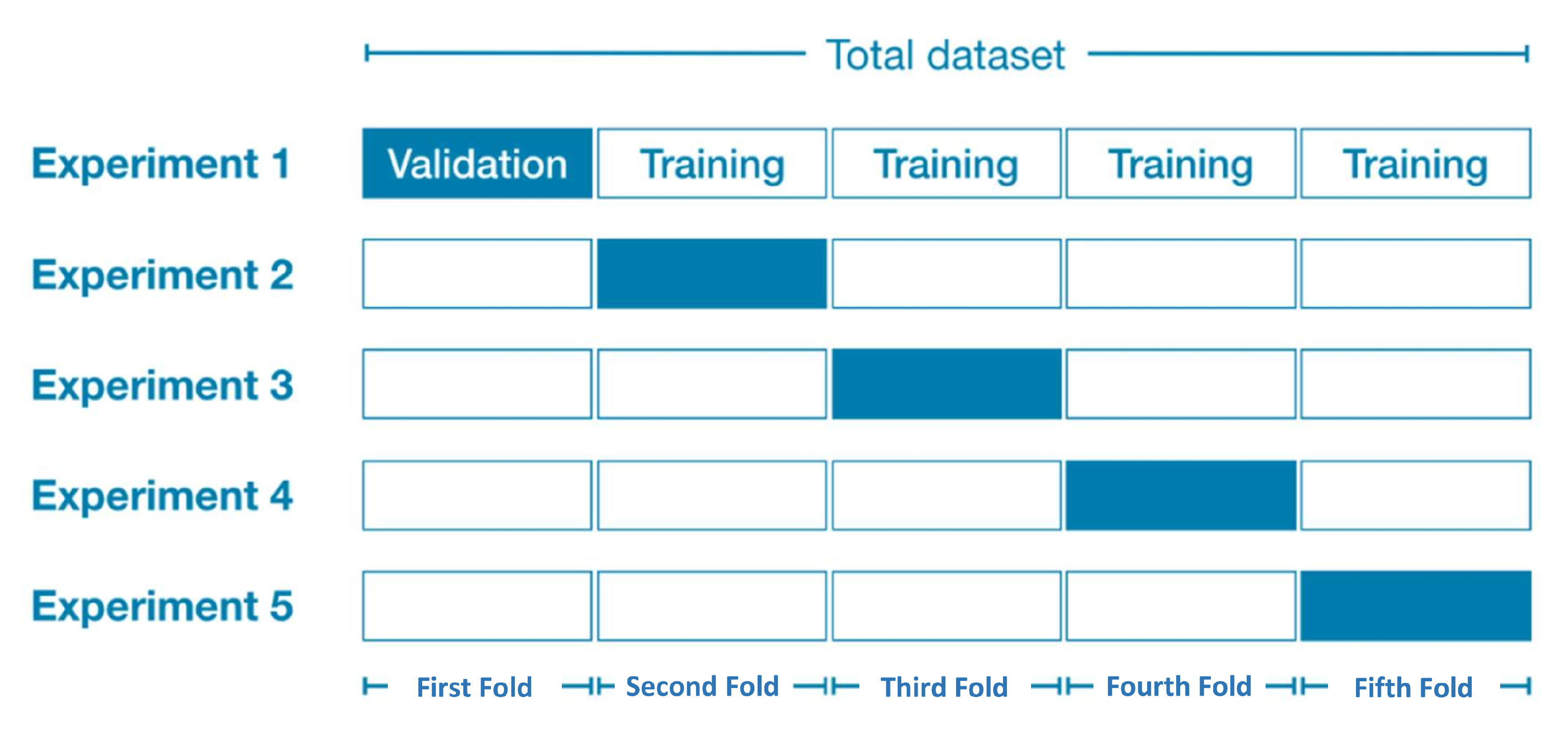
| Experiment | Two-Class | Five-Class | ||
|---|---|---|---|---|
| Accuracy | Error | Accuracy | Error | |
| Experiment 1 | 0.9930 | 0.0070 | 0.9820 | 0.0180 |
| Experiment 2 | 0.9942 | 0.0058 | 0.9950 | 0.0050 |
| Experiment 3 | 0.98750 | 0.01250 | 0.9907 | 0.0093 |
| Experiment 4 | 0.99440 | 0.00560 | 0.9929 | 0.0071 |
| Experiment 5 | 0.99320 | 0.00680 | 0.9966 | 0.0034 |
| Average | 99.25% | 0.75% | 99.14% | 0.86% |
| Research | Accuracy | IF % |
|---|---|---|
| K. Taher et al. 2019 [12] | ≈83.7% | 117.3% |
| X. Gao et al. 2019 [13] | ≈85.2% | 115.2% |
| S. Sapre et al. 2019 [14] | ≈78.5% | 125.1% |
| M. Chowdhry et al. 2017 [15] | ≈94.6% | 103.8% |
| Q. Niyaz et al. 2016 [16] | ≈88.4% | 112.3% |
| I. Yadigar, et al. 2016 [17] | ≈91.7% | 108.0% |
| Proposed Method | ≈98.2–99.3% | ____ |
| Research | Data | Accuracy | IF % |
|---|---|---|---|
| G. Bendiab et al. 2020 [9] | Zero-Day Malware | ≈94.50% | 105.0% |
| R. Shire et al. 2019 [10] | Zero-Day Malware | ≈91.32% | 107.5% |
| I. Baptista et al. 2019 [11] | Ransomware filetypes | ≈94.10% | 104.4% |
| S.Jan et.al 2019 [18] | CICIDS Dataset | ≈93.0% | 106.7% |
| M. Roopak et al. 2019 [19] | CICIDS Dataset | ≈92.0% | 107.9% |
| C. Ioannou et al. 2019 [20] | Simulated Dataset | ≈81.0% | 122.5% |
| O. Brun et al., 2018 [21] | Real-Time Dataset | ≈75.0% | 132.4% |
| V. Thing et al. 2017 [22] | AWID Dataset | ≈98.0% | 101.3% |
| P. Shukla et al. 2017 [23] | Simulated Dataset | ≈75.0% | 132.4% |
| E. Hodo et al. 2016 [24] | DoS Dataset | ≈99.0% | 100.3% |
| C. Kolias et al. 2016 [25] | AWID Dataset | ≈92.0% | 107.9% |
| Y. Li et al. 2015 [26] | KDDCUP Dataset | ≈92.0% | 107.9% |
| Proposed Method | NSL-KDD Dataset | ≈98.2–99.3% | ____ |
Publisher’s Note: MDPI stays neutral with regard to jurisdictional claims in published maps and institutional affiliations. |
© 2020 by the authors. Licensee MDPI, Basel, Switzerland. This article is an open access article distributed under the terms and conditions of the Creative Commons Attribution (CC BY) license (http://creativecommons.org/licenses/by/4.0/).
Share and Cite
Abu Al-Haija, Q.; Zein-Sabatto, S. An Efficient Deep-Learning-Based Detection and Classification System for Cyber-Attacks in IoT Communication Networks. Electronics 2020, 9, 2152. https://doi.org/10.3390/electronics9122152
Abu Al-Haija Q, Zein-Sabatto S. An Efficient Deep-Learning-Based Detection and Classification System for Cyber-Attacks in IoT Communication Networks. Electronics. 2020; 9(12):2152. https://doi.org/10.3390/electronics9122152
Chicago/Turabian StyleAbu Al-Haija, Qasem, and Saleh Zein-Sabatto. 2020. "An Efficient Deep-Learning-Based Detection and Classification System for Cyber-Attacks in IoT Communication Networks" Electronics 9, no. 12: 2152. https://doi.org/10.3390/electronics9122152