Bus Dynamic Travel Time Prediction: Using a Deep Feature Extraction Framework Based on RNN and DNN

Abstract

Travel time data is an important factor for evaluating the performance of a public transport system. In terms of time and space within the nature of uncertainty, bus travel time is dynamic and flexible. Since the change of traffic status is periodic, contagious or even sudden, the changing mechanism of that is a hidden mode. Therefore, bus travel time prediction is a challenging problem in intelligent transportation system (ITS). Allowing for a large amount of traffic data can be collected at present but lack of precisely-conducting, it is still worth exploring how to extract feature sets that can accurately predict bus travel time from these data. Hence, a feature extraction framework based on the deep learning models were developed to reflect the state of bus travel time. First, the study introduced different historical stages of bus signaling time, taxi speed, the stop identity (ID) of spatial characteristics, and real-time possible arrival time, signified by fourteen spatiotemporal characteristic values. Then, an embedding network is proposed to leverage a wide and deep structure to mate the spatial and temporal data. In order to meet the temporal dependence requirements, an attention mechanism for a Recurrent Neural Network (RNN) was designed in this research in order to capture the temporal information. Finally, a Deep Neural Networks (DNN) was implemented in this research in order to achieve the dynamic bus travel time prediction. Two case studies of Guangzhou and Shenzhen were tested. The results showed that the performance of the algorithm was more efficient than that of the traditional machine-learning model and promoted by 4.82% compared to the deep neural network applied to the initial feature space. Moreover, the study visualized the weighted cost of attention on the bus’s travel time features during a certain running state. Therefore, the study demonstrated the proposed model enabled to understand the characteristic data of transit travel time with visualization.

1. Introduction

Bus travel time prediction is an important component of an intelligent transport system (ITS). The precise capturing of real-time travel information facilitates the choice of an optimal route by a traveler. Additionally, with unforeseen events occurring, traffic managers adjust departure schedules in real time to ensure the service quality of a system [1,2]. Nevertheless, the travel time of the same bus route in the same city is dynamic due to the nature of bus operation because of frequent traffic congestion, traffic accidents, and road construction. Therefore, it is necessary to focus on a real-time and dynamic bus travel time prediction model in depth in order to further improve traffic efficiency.

Bus travel time prediction has three dependencies. (1) Time dependence [3]: Due to the strong periodicity of passenger demand, bus scheduling also has a certain periodicity. Moreover, bus travel time also depends on the tendency of recent historical travel times. (2) Spatial dependence: The travel time of a particular line is influenced not only by the current traffic state variables of the running line but also by the traffic state variables of the entire bus line [4]. (3) Exogenous dependence: Some exogenous variables, weather conditions, and emergencies may have a great impact on traffic timing prediction [5]. However, driven by big traffic data, a challenge arises: can one gain broad utilization of the latent knowledge hidden in big traffic data in order to predict bus travel time?

Currently, the original statistical-based parameter models (such as K-Nearest Neighbor (KNN) or ARIMA) or machine learning models (such as Support Vector Machine (SVM)) are experiencing more and more difficulty in meeting the requirements of big data in some areas, while the research field of neural networks is active [6,7]. Recently, the neural network shallow prediction model has been used in most scenarios [8]. However, these models have limitations when dealing with large historical data sets and complex nonlinear functions [9].

Deep learning integrates multi-layer architecture and regression to extract inherent features in an end-to-end way. Based on the analysis of a large amount of real-time and historical traffic data, a deep neural network model can deal with the nonlinear characteristics of traffic data and obtain more precise prediction results [10]. However, real-time dynamic bus travel time prediction is very complex, and it involves complex space-time features [11,12]. Moreover, the potential traffic status and traffic events are in a hidden mode. Therefore, the development of a deep learning model is not well suited to capturing the deeper characteristics of bus travel time effectively [13].

For the critical issue of interpreting the space-time features of bus travel time, data-driven methods and neural network methods have been doubted to have this ability [5]. However, there have been a few research literature references that have focused on the diverse traffic features affecting the final prediction of bus travel time. Therefore, this research aimed to explore a new methodology for handling a large number of spatio-temporal features by using deep learning models for the prediction of bus travel time.

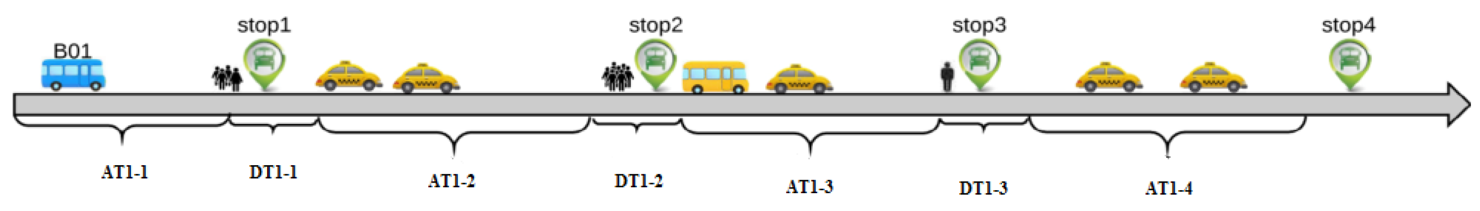
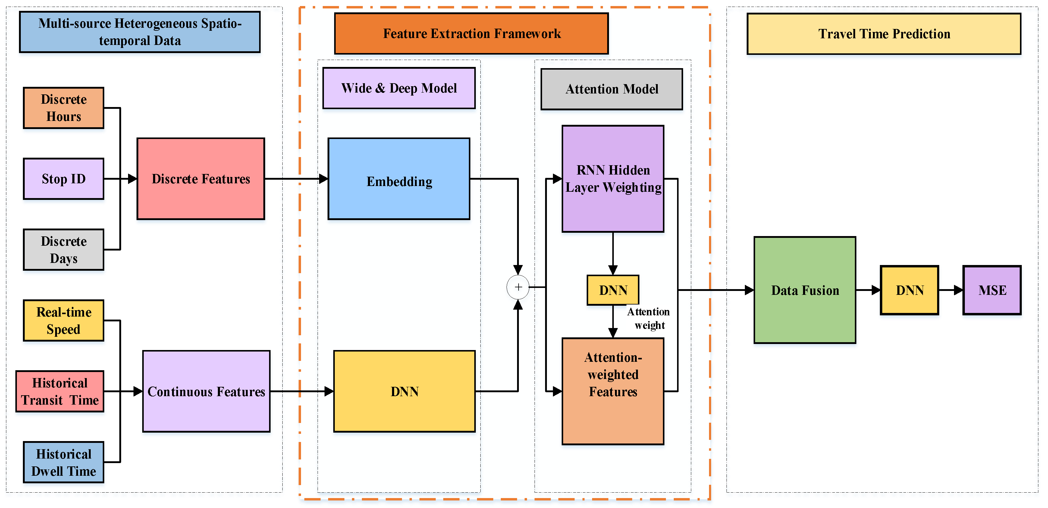
In order to solve the problem of focusing on big data feature extraction for bus travel time prediction, in this study, a dynamic real-time bus travel time prediction method was proposed based on a deep learning feature extraction framework and data fusion. In this research, bus travel times were divided into running times and dwelling times, and Global Positioning System (GPS) speeds were added for taxis and buses, as well as travel times based on real-time speeds in order to predict dynamic bus travel times, as indicated in Figure 1. In summary, the main contributions of the proposed approach are those reported below.

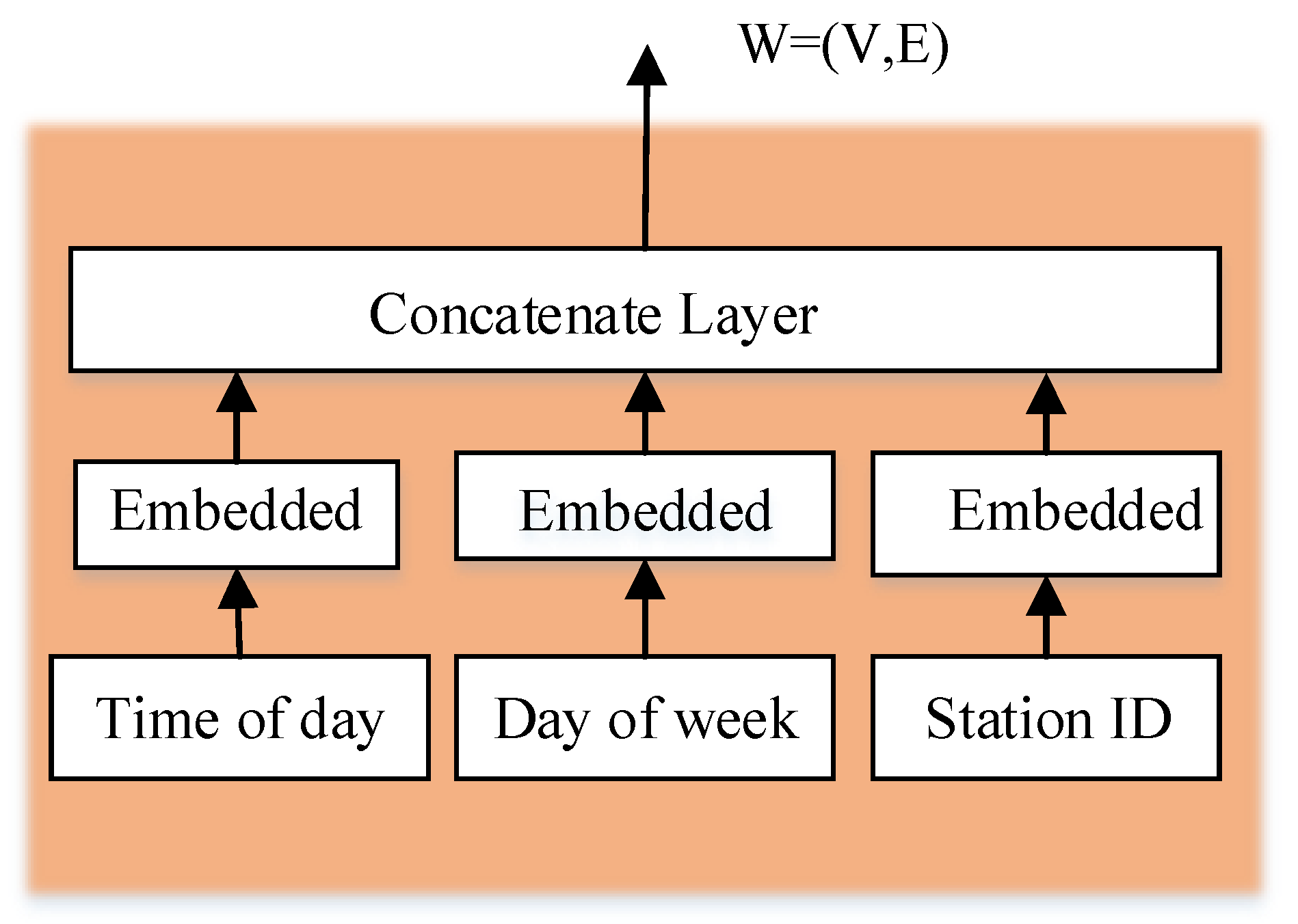
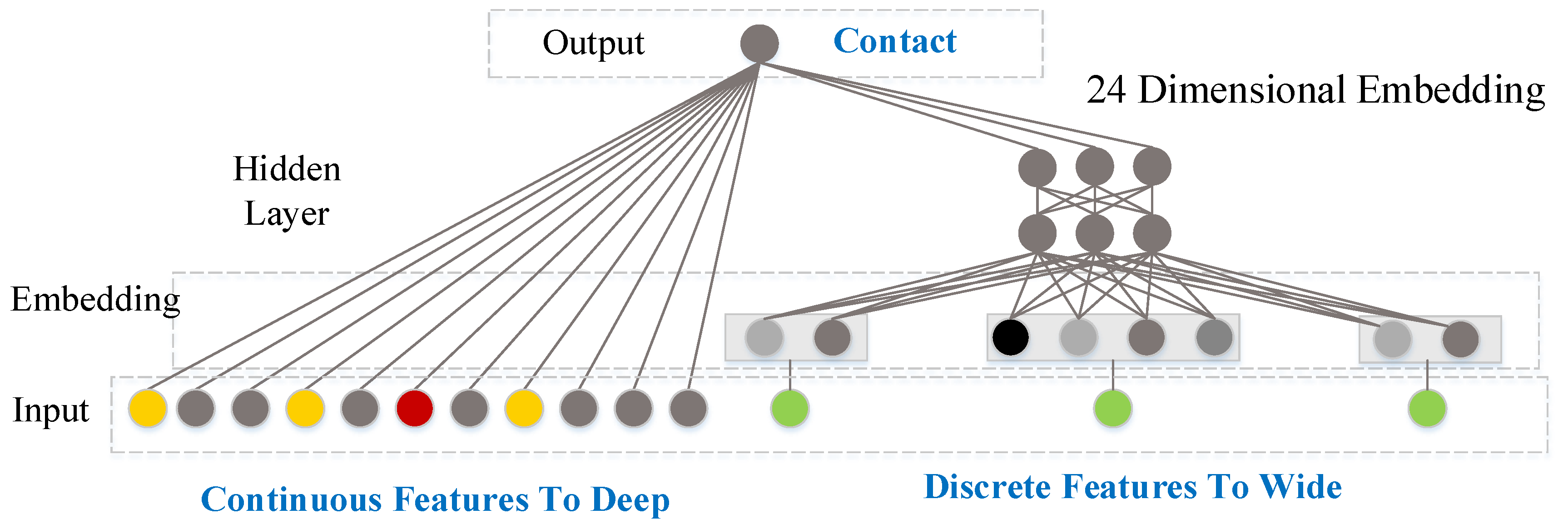
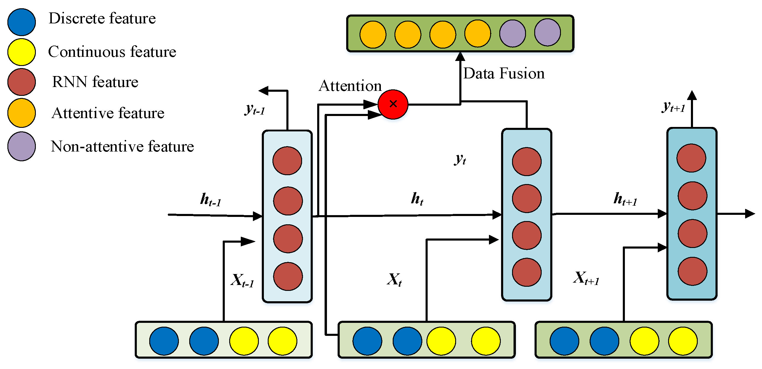
Based on the prediction of bus travel time, in this research, a new heterogeneous feature extraction framework was proposed based on the recurrent neural network (RNN) model of embedding wide and deep (WD) and an attention mechanism. The framework was proposed in order to gain a deep understanding of the spatio-temporal features and intrinsic connections of the characteristics related to bus travel time and to visualize the connections.

Fourteen spatial and temporal features were introduced, including stop Identities (IDs) as special characteristics, bus dwelling times at different historical levels, real-time GPS bus speeds with real-time possible transit times obtained based on real-time bus speeds as temporal features. These features have not been analyzed together in previous surveys. Lastly, multiple super positions of the RNN and Deep Neural Networks (DNNs) were employed to reduce the residual heterogeneous data fusion and real-time dynamic bus travel time prediction. A novel system for real-time dynamic bus travel time prediction was offered.

To verify the model’s stability and generalization ability, the model was tested on the datasets of the Guangzhou No. 226 bus and the Shenzhen No. 113 bus. These buses ran along the main roads in large urban centers. Both of the experiments achieved good results. Other studies never tested their models in different cities.

2. Literature Review

Ever since the rapid development of deep learning methods occurred, the potential for processing large-scale high-dimensional data has been maturing [3,10,14,15,16,17,18].

Recurrent Neural Network (RNN), which is a distinctive construction of deep learning models, is widely used to solve sequence problems [19]. This type of network extends a DNN by repeatedly connecting hidden layers in different timestamps. In this network structure, memory units can dynamically model sequence data. Lately, some studies in the field of transportation has begun to seek RNN to solve the problem of time series predictions, such as traffic flow [20], traffic speed [10], and travel time prediction [21]. Petersen et al. (2019) and He et al. (2020) developed an RNN architecture for the prediction of bus travel times. They demonstrated that the network could capture long-term time dependencies in traffic data, as shown in

Table 1. A comparison of travel time prediction approaches.

Paper	Model	Feature Extraction	Classification	Factors			Number of Cities	Size of Cities
				AVL	Speed	Dwelling Time
[23]	SVM, ANN	Cluster	Temporal	Yes	Bus	Historical mean	1 city	megacity
[4]	SVM ANN KNN	No	Temporal	Yes	Taxi	Predicted	1 city	megacity
[22]	CNN RNN	No	Spatio-temporal	Yes	No	No	1 city	metropolis
[6]	RNN	Cluster	Temporal	Yes	No	Historical mean	1 city	megacity
[5]	DNNS	PCA, Cluster	Spatio-temporal	Yes	No	No	1city	metropolis
Ours	RNN DNNs	Embedding Wide and- Deep Attention	Spatio-temporal	Yes	Bus and taxi	Multiple stages	2 cities	Megacities

Note: AVL means automatic vehicle location.

[6,22].

Deep Neural Networks (DNN) has deep fully connected neural layers. An individual DNN does not require the manual extraction of features, and it learns in a supervised way. For our specific problem, the factors that caused congestion, queue delays, and traffic flow came from the fuzzy interaction with complex features. DNN is a multi-layer deep structure that can extract features from data and reveal important potential or hidden structures. Furthermore, DNN provides a powerful and new way to learn how these features interact. Abdollahi et al. (2020) trained a deep, multi-layer perceptron to predict bus travel time [5].

Although the exploration of deep learning models with applications to bus travel time prediction has achieved delightful results, there are still some limitations in these fields. A comparison of the latest bus travel time prediction studies is shown in Table 1.

There are few existing studies on bus travel time prediction using deep learning methods. It has been even rarer to study real-time dynamic bus travel time prediction. In the only studies, although the deep learning methods had a powerful ability to handle large amounts of data and high-dimensional data, the gap between large-scale data and its shallow structure, the gap between full connectivity and rich features [5,13], and the hidden patterns of potential traffic states and traffic events made it difficult for the above models to derive representative features from the rich feature data set. In other words, there has been a lack of systematic, perfect, and in-depth feature learning. Therefore, it is necessary to develop a deep-seated deep learning architecture that fully reflects the features of bus travel time prediction.

The existing studies of the prediction of bus travel time with feature learning still belong to the category of shallower feature learning. Examples include geospatial feature analysis, principal component analysis (PCA), and unsupervised learning algorithms (K-Means) to extract spatial features, and a deep-stacked auto-encoder (SAE) to represent low-dimensional features [5,23]. Using the deep structure of a Recurrent Neural Network (RNN) in time, the historical sequence information was automatically remembered in the model structure [6,22]. The spatial features of the data were extracted from the Convolutional Neural Network (CNN) for use by the Long Short-Term Memory (LSTM) network [22]. DNNs were also used to predict bus travel times after feature extraction [5]. However, most of the research on bus travel time has been shallow in terms of the feature learning structures [5,6,23], lack of feature learning [4,22], or lack of feature learning depth and related breadth. Therefore, it is of great significance to develop a deep feature extraction structure that fully reflects the characteristics of travel time.

The study proposed a neural network that integrated embedded, wide and deep algorithm, and attention mechanisms, and introduced them into a dynamic bus travel time prediction model for design. The extraction framework made use of the non-static space-time correlation existing in urban public transport networks and discovered complex models that traditional methods could not capture. Our study also visualized the RNN model to interpret the impact of various spatial-temporal features on the prediction of dynamic bus travel times, which challenged the traditional neural network approach in the public transport field.

3. Prediction Model

3.1. Feature Extraction Framework

The underlying feature extraction framework was proposed. The framework was composed of Embedding, Wide and Deep, and Attention models.

3.1.1. Embedding

One-hot encoding is one of the most common methods used in dealing with discrete data. Taking Wednesday as an example, it is the third day of a week, and (0, 0, 1, 0, 0, 0, 0) is used to represent three out of seven. One-hot encoding treats each dimension independently, but these representations might not be capable of catching the similarity of each variable; for example, Saturday and Sunday during peak periods might be similar. Additionally, one-hot encoding is too sparse, which is difficult for a deep learning model to deal with [24]

Embedding is a particularly effective method to solve the problems mentioned above, which can be formalized into the following expression:

$$embedding=map\left(X\in R^{N\times 1}\to X_E\in R^{N\times d}\right),$$

where N denotes the words, d is the embedding size, X is the feature, $X_E$ is the recoded features, and R is the data feature set.

Similar to the data structure mentioned in Section 3.2, the features hours (time of data), day (day of week), and distance, which was used as the station ID instead of bus travel distance, were discrete data features. In order to capture more similarity for each feature, the study implement an embedding model for each feature, as shown in Figure 2.

3.1.2. Wide and Deep

The bus travel time prediction task included both discrete features and continuous features. The dimensions of the discrete features were much smaller than those of continuous features, and the model would be more susceptible to the impact of continuous data if these features were directly input into the deep model for training. To solve this problem, our study were inspired by the designation of Wide and Deep, shown in Figure 3, for which the core idea was to combine the memory ability of the linear model with the generalization ability of the deep model. In this study, discrete features were applied, such as hours, day, and distance to the wide side, and continuous features were applied to the deep side.

a.

The Wide Component

Since the wide side had a high memory ability, it could be used to map the interrelationships after the embedding of discrete features turned into continuous features. Therefore, the discrete features were input into the wide side.

The wide side emphasized features that had often co-occurred in the past, also known as “frequent co-existence features.” For example, “Monday”, “7:30–9:30,” and “station 2–3” often appeared together. The relationship between these three terms allowed us to explain why they occurred so often together. In fact, the memory could be effectively captured by adding interaction items to a broad learning model. The wide side is a generalized linear model for which the form is

$$embeddin{g}_{fd}=W_{V\times N}^T\times one\_hot\left(f_d\right)+b$$

(1)

where, $embeddin{g}_{fd}$ denotes the predicted discrete outputs, which were treated as traffic state features, W is a $V\times N$ matrix, and V is the set size of the corresponding discrete features. $one\_hot\left(f_d\right)$ is the one-hot encoding corresponding to the discrete features.

b.

The Deep Component

Generalization is the use of new feature interactions that have occurred rarely or never in historical data, such as “V3 = 40.1” rarely co-occurring with “DT1 = 3” at the same time. Therefore, the wide side could not be used to predict situations that had occurred rarely or never in historical data. However, deep neural networks could find correlations between invisible features.

The deep side had strong feature generation ability, so continuous features were input into the deep side. This allowed the model to capture correlations between different continuous features. The learning model for the expression of continuous features can be expressed as follows:

$$featur{e}_{fc}=W_{M\times N}^T\times f_c+b$$

(2)

where, $featur{e}_{fc}$ represents the Continuous features in the bus operation data, W is the vector $M\times N$, $M$ is the size of the continuous features, $N$ is the size of the embedding, $f_c$ is the hidden layer of the neural network, and $b$ is the offset.

c.

Joint Training of the Wide and Deep Model

Finally, the features calculated from the two branches were spliced together to obtain the features extracted from the original data. These features can be expressed as

$$featur{e}_f=embeddin{g}_{fd}\oplus featur{e}_{fc}$$

(3)

where, $featur{e}_f$ is formed by combining discrete features and continuous features, and ⊕ is the split joint.

3.1.3. Attention Mechanism

In this study, the attention mechanism was introduced into the task, and our attention-based RNN model that used spatial-temporal features to predict dynamic bus travel times and capture the importance of spatial-temporal features at different locations was proposed.

The attention model performed element-wise multiplication with each feature matrix to obtain a weighted feature matrix, as shown in Figure 4:

$$attn\_featur{e}_t=attn\otimes featur{e}_t.$$

(4)

The goal of the attention model was to learn an attention weight matrix $attn\_feature{T}_t$. In this study, an RNN model was proposed in which $h_t$ was used to learn weights at different states. Each element could be interpreted as the relative importance of $T^f\left(featur{e}_{f}atT\right)$. The activation function $sigmoid$ between the output and the hidden layer could limit the output to between 0 and 1:

$$attn\_feature{T}_t=sigmoid\times \left(W^T{h}_t\left(T^f\right)+b\right)$$

(5)

In the formula, W is a $T^f$ matrix, and $h_t$ is a mapping between the input and hidden neurons. In this study, Long Short-Term Memory (LSTM) or Gated Recurrent Unit (GRU) was used in a fully-connected RNN network. Then the spatial-temporal matrix $T^f$ of the historical bus journey point by point was multiplied with the attention matrix $attn\_feature{T}_t$ (as shown in Formula (2) to obtain a weighted bus journey time matrix for further learning. Therefore, the final attended feature was

$$attn\_T_{rnn}=attn\_feature{T}_t\otimes T^f$$

(6)

In the formula, $attn\_T_{rnn}$ is the weighted eigenvector, and ⊗ represents the multiplication of the corresponding elements one by one.

The RNN was used to model the series data, and the RNN hidden features were used to weigh the features. The formation process of the weighted travel time matrix is shown in Figure 5.

3.2. Dynamic Bus Travel Time Prediction

The bus travel time prediction procedures underlying are formed by embedding module, Wide and Deep module, RNN and DNN.

Step1: embedding model compresses and encodes discrete data, extracting correlations between discrete features.

Step2: since the wide side had a high memory ability, it was used to map the interrelation ships after the embedding of discrete features turned into continuous features. The deep side captures correlations between different continuous features. The features calculated from the two branches were spliced together to obtain the features extracted from the original data. The wide and deep module that fused discrete and continuous features are shown in Figure 6.

Step3: all of the features were weighted by the attention module. The weighted features were fed into the RNN and DNN models.

DNN is a fully connected deep learning model, which has better ability to obtain the optimal solution. However, there is an insoluble problem with fully connected DNN: it is impossible to model changes in time series. In a normal fully connected network, the hidden layer of DNN can only receive the input at the upper layer at the current moment, while in RNN, the output of neurons can act directly on itself in the next period. In other words, the hidden layer of a recursive neural network can not only receive the input of the previous layer, but also get the input of the current hidden layer at the previous moment. The significance of this change is that it makes the neural network capable of historical memory [26]. In principle, an infinite amount of historical information is well suited for tasks with long-term relevance, such as speech and language. The memory function of RNN is particularly suitable for memorizing and mining sequence data. The multiple combinations and superposition of DNN and RNN can capture the characteristics of the permissible sequence in bus travel time prediction and obtain the optimal solution. Meanwhile, the residual errors can be eliminated by multiple combinations and superposition.

Then Mean Squared Error (MSE) was used in this study to train the model to predict the bus dynamic travel time, as shown in Formula (7):

$$los{s}_t=\frac{1}{2}{\left|targe{t}_t-\widetilde{targe{t}_t}\right|}^2,$$

(7)

In the formula, $los{s}_t$ is a loss function, $targe{t}_t$ is the real travel time at time t, and is the predicted value at time t.

The model was built to be end to end, and all of the parameters in the model were trained together. Our general training process is listed as Algorithm 1.

Algorithm 1: Process for Model Training
1	Input:
2	Discrete data fd in the training dataset
3	Continuous data fc in the training dataset
4	Travel time targett in the training dataset
5	Output:
6	Step 1: Initialize all parameters
7	Step 2: Feature extraction
8	Step 3: Feed fd to the Embedding model to obtain embeddingfd
9	Step 4: Feed fc to the DNN model to obtain featurefc
10	Step 5: Concatenate all {embeddingfd, featurefc} as featuref
11	Step 6: For all states in a series of traffic data, do
12	SAMPLES = [[f1,f2,f3,…,fT]]
13	End for stage I feature extraction
14	Training Algorithm
15	Repeat
16	Step 7: Randomly choose a batch of samples in SAMPLES
17	For each state of the above
18	Get RNN output outputt
19	Get Attention features attn_featuret
20	End of stage II feature extraction
21	Concatenate both {outputt,att_featuret}
22	Get forecasted travel time targett
23	Compute loss on and targett using the mean standard error
24	Back propagation
25	Until convergence
26	End training

4. Data Collection and Feature Definition

4.1. Data Collection

We evaluated our approach using a large number of buses and taxi GPS data, as well as the bus Automatic Vehicle Monitoring (AVL) data collected by the Transport Department of Guangzhou and Shenzhen in the south of China, which are metropolises with populations of over 14.9 million people and 13.2 million people, respectively.

The bus travel time prediction could be divided into a main road with a signal and a road without a signal. Our experiment in Guangzhou and Shenzhen included different signal periods for multiple intersections connected to each other, which was more challenging for the accuracy of urban main road prediction [27].

To test the No. 226 Bus line in Guangzhou City (23.2 km, 28 stations), the dates for 27 sections and the corresponding areas were collected from 5 October 2014, to 9 November 2014. The No. 226 bus ran through the artery roads (such as Huangpu Road and Dongfeng Road). The running time of the vehicles was 6:00–22:00, and the departure time was 10 min.

The Shenzhen data set used data for the No. 113 bus (19.5 km, 23 stations) with 23 sections and the corresponding areas collected from 20 March 2018, to 5 August 2018. The buses ran through the main road, ShenNan Avenue. The running time of the vehicles is 6:10–23:00, and the departure time was about 4–8 min.

4.2. Features and Definition

Firstly, the main reason why existing estimation approaches could not achieve excellent accuracy is the fact that the travel times are impacted by various factors, such as different weather conditions [28,29], temporal variation of peak and off-peak hours [4,30,31], boarding passenger information [32,33,34], and real-time traffic conditions [35,36]. Some work focus on analyzing the impacts of different factors. In the study of He [37], the traffic state reports from Twitter information is added as additional data support to predict travel times. The results show that knowing real-time traffic condition helps to increase the estimation accuracy. From the analysis results of the above studies, we can observe that the traffic conditions are uncertain and important for travel time prediction [38]. However, bus GPS data are usually infrequent. Especially, the penetration rate of buses in the traffic network is low at low speed. It is less insensitive to irregular traffic conditions than taxis. It can be observed that only limited studies exist that analyses the influence of real-time traffic flow conditions on bus travel times and the correlation between them [4].

Secondly, the data of Shenzhen city is of 2016. In 2016, the working hours of bus lanes in Shenzhen were from 7:30 am to 9:30 am and from 17:30 pm to 19:30 pm on weekdays (except statutory holidays).Taxes are usually allowed to travel on bus lanes during non-bus lane working hours. In addition, in the field observation of taxi operation, it is found that sometimes passengers will park in the bus lane when getting on or off the taxi. As a result, taxis sometimes run on bus lanes.

Moreover, the data of Guangzhou comes from the time when bus lanes have not been implemented. Therefore, at that time, buses and taxis were traveling together. Therefore, bus GPS and taxi GPS were taken into account when considering the traffic status. Additionally, Different studies have different definitions of real-time. Nikolas Julio [39] defined the dynamic travel time prediction as 10 min when studying the use of traffic shock waves and machine learning algorithms to predict bus speed in real time. Qichongb [40] Predicts bus real-time travel time basing on both GPS and RFID data based on the assumption that the traffic flow keeps the same level in an interval of 30 min although he collects GPS data every 30 s. Hans [41] forecasts Real-time bus route state using particle filter and mesoscopic modeling with four loop detectors installed along the same corridor. Archived data provides access to volume and occupancy information collected approximately every minute. In order to predict the dynamic bus travel time, this paper adds the real-time GPS speed data of the bus every 20 s to the feature for dynamic bus travel time prediction, which effectively improves the prediction accuracy.

Allowing for the data of Shenzhen city based on 2016-year when the exclusive hours of bus lanes in Shenzhen were from 7:30 am to 9:30 am and from 17:30 pm to 19:30 pm on weekdays (except statutory holidays). Besides, taxes are indeed allowed to travel on bus lanes during non-exclusive-bus operating hours. In addition, in the field observation of taxi operation, it is found that sometimes passengers will park in the bus lane when getting on or off the taxi. As a result, taxis always run on bus lanes. Moreover, the fundamental data derived from bus GPS and taxi GPS were taken into account in the paper, which are assumed to represent the traffic status of the PT and road transit, respectively.

We selected fourteen characteristic data sets related to bus travel time prediction, including discrete data, continuous data, spatial data, and time data, as shown in

Table 2. Features and definition.

Features	Data type	Temporal/Spatial	Definition
dt1	Continuous	Temporal	Average bus dwell time within 30 min.
dt2	Continuous	Temporal	Average bus dwell time in 30 min at this point in the last week.
dt3	Continuous	Temporal	Average bus dwell time within 30 min on the same day of the last week.
at1	Continuous	Temporal	Average bus travel time within 30 min.
at2	Continuous	Temporal	Average bus travel time within 30 min of the last week.
at3	Continuous	Temporal	Average bus travel time within 30 min on the same day of the last week.
V1	Continuous	Temporal	Average velocity of the probe vehicles within 5 min.
V2	Continuous	Temporal	Average velocity of the probe vehicles in 5 min at this point in the last week.
V3	Continuous	Temporal	Average velocity of the probe vehicles within 5 min on the same day of the last week.
Real-time speed	Continuous	Temporal	The real-time bus speed was used to reflect the real-time traffic status in the bus lane.
Possible time	Continuous	Temporal	The distance between stops divided by the real-time speed of the bus
Day	Discrete	Temporal	Day of the week, day = {1,2,3,4,5,6,7}.
Hours	Discrete	Temporal	Hours of the day, hours = {8,9…,20}.
Stop-ID	Discrete	Spatial	This reflected the spatial relationship between stops and the impact of different stops on the bus travel time prediction.

. In this paper, the features of exited studies is refined into multiple stages, and expanded to the speed of bus and taxi rather than that of one kind vehicle, thus making it more comprehensive to reflect the traffic state.

The existed studies on dynamic travel time using deep learning model, especially the dynamic bus travel time, has not yet been considered. Therefore, based on the above eigenvalues, we added the real-time speed collected within 20s of the bus prediction time into the deep learning model proposed in this paper to predict the dynamic bus travel time.

5. Evaluation

5.1. Establishment of the Experiment

5.1.1. Platform Configuration

The experimental platform hardware components used in this study were an Intel Core i7 8700 @3.2 GHz and 32G DDR4 Memory. The platform software was Centos7.5. Our experiment was operated using Python 3.6.8 and TensorFlow 1.10.0.

The experimental data can be found in Section 3, and the data features are shown in Table 2.

5.1.2. Missing Data

In the process of collecting data, missing data could not be avoided. In our experiments for this study, the records with missing values were discarded because of the use of an RNN, but all the states for a whole line were not discarded for the study. Instead, our study put the site information in as a discrete feature on the wide side for feature learning, which has been talked about previously. Therefore, for the entire bus travel time sequence, there may have been a sequence, such as 1-2-5-8-10, for which a station with missing data was dropped.

5.1.3. Hyper Parameters

In the experiment, the size of embedding for the research was set to four at the wide side, and the number of hidden DNN nodes at the deep side was set to 16. Finally, the features were concatenated. Each state was converted to 28-dimensional features.

5.2. Evaluation Criteria

Three metrics are often used to evaluate the performance of traffic prediction models. They are the mean absolute percentage error (MAPE) [10], mean absolute error (MAE) [4,10,13], and root mean square error (RMS) [10,13]:

$$MAE=\frac{1}{n}{\displaystyle {\sum }_{i=1}^n}\left|x_i-{\tilde{x}}_i\right|,$$

(8)

$$MAPE=\frac{100}{n}{\displaystyle {\sum }_{i=1}^n}\left|\frac{x_i-{\tilde{x}}_i}{x_i}\right|,$$

(9)

$$RMSE=\sqrt{\frac{1}{n}{\displaystyle {\sum }_{i=1}^n}{\left(x_i-{\tilde{x}}_i\right)}^2},$$

(10)

where, N is the number of samples, i is the number of stations, $x_i$ is the real bus travel time, and ${\tilde{x}}_i$ is the predicted bus travel time.

The MAE and MAPE are indicators of regression tasks. Compared with the MAE and MAPE, the RMSE is more sensitive to outliers, and it can amplify larger prediction deviations. It is often used to compare the stability of different prediction models. The MAPE provides prediction errors based on the percentage difference between observed and predicted bus travel times as a measure of the prediction accuracy of the statistical prediction methods. These performance indicators provide a deep understanding of the nature of prediction errors [10].

5.3. Experiment Results

This section describes the evaluation of the accuracy of our approach for this study based on six types of experiments with our proposed model compared to the existing models.

5.3.1. Different Method

To study different methods of accuracy, the following results were compared for the test set of MAPE indicators in this research: The historical average estimate HAV, using only historical information and not joining the floating vehicle average speed information SVR1, historical information with the floating vehicle average speed SVR2 and a prior probability distribution of the bus travel time, the use of Bayesian theory to modify the SVR2-Bayes theorem of the SVR2 experiment results, the linear model, a neural network based on depth within the DNN [5] and RNN [6], and our proposed methods. See

Table 3. Results for GuangZhou261.

Error Index	HAV	SVR	SVR1	SVR 2	ANN	SVR 2-Bayes	SVR 2-Bayes2	Our Study
MAPE (%)	18.5	17.98	17.98	16.4	17.23	14.93	14.29	8.43

and Figure 7 [5,6].

Table 3 indicates that the DNN [5] and RNN [6] represented relatively advanced artificial intelligence algorithms. The DNN had nearly 5% more absolute promotion than the SVR2-Bayes2 model did. After replacing the model with the RNN, the MAPE could be further reduced by capturing the interdependence between different sites, indicating that the spatial-temporal relationship between sites had a certain impact on the prediction accuracy. However, the RNN itself did not pay attention to the importance of different features in different states. Therefore, our study combined the RNN with Wide and Deep and attention mechanisms to form a feature extraction framework. The accuracy of the proposed RNN network was further reduced by 0.5% and relatively improved by 5% compared with the RNN network alone.

Based on Guangzhou PT center dataset, in order to study the changes in the travel time at different times for each station, the predicted and true values of the bus travel time model for 8:00 AM were randomly selected. It can be seen from

Table 4. MAPE values for different methods in different periods.

	MAPE	SVR2 (%)	SVR2-Bayes (%)	SVR2-Bayes2 (%)	Our Study (%)
Time
Morning (08:00–09:00)		15.99	14.21	13.83	9.51
Evening (17:00–19:00)		16.24	13.69	13.62	6.43
Flat peak		14.37	14.38	12.25	5.21

that our model could reduce the MAPE by 4–7% compared with svr2-bayes2, indicating that our algorithm had a good performance during the peak or flat peak times.

5.3.2. Different Dataset

The MAE and MAPE are indicators of regression tasks. For different scenarios, we use MAE and MAPE two standards to evaluate the error. First, for a complete bus line, compare the data sets of Guangzhou and Shenzhen with RNN, DNN and our own algorithm, and use MAE to evaluate the error time to compare the operation of the entire line. This is important for traffic managers or bus scheduling and dispatching personnel. The MAPE provides prediction errors based on the percentage difference between observed and predicted bus travel times as a measure of the prediction accuracy of the statistical prediction methods. Then, for the morning peak, evening peak and peace peak, we use MAPE for comparison and evaluation of the stability of different prediction models. These performance indicators provide a deep understanding of the nature of prediction errors. The results as below.

(1)

With using the data for the No. 261 bus in Guangzhou and No. 113 bus in Shenzhen, we verify the generalization performance of our model. The results showed that the proposed algorithm in this research had better performance for the whole routes than the DNN or the RNN for both the Guangzhou and Shenzhen datasets, as shown in Figure 7.

(2)

We chose the peak period of the working day with a more complex traffic state and the flat peak period with a simple traffic state as the research period, and we compared the algorithms. It can be seen from

Table 5. Comparison of the results of the model for Guangzhou and Shenzhen.

	MAPE	Guangzhou (%)	Shenzhen (%)
Time
Morning (08:00–09:00)		10.79	8.74
Evening (17:00–19:00)		9.11	9.33
Flat peak		8.17	7.97

that for the maximum morning rush hour of the MAPE in Guangzhou, the error of the one-hour bus journey time was about 6.5 min. For the maximum evening peak of the MAPE in Shenzhen, the error of the one-hour bus journey time was about 5.6 min, which indicated that this model had good generalization ability, and it solved the problem that the proposed deep learning algorithms were suitable for the traffic states of different cities.

5.3.3. Real-Time Bus Speed Information for Prediction

In order to get closer to the application scenario, our study divided their model into two scenarios in the prediction process. The two scenarios comprised a model based entirely on historical data and a model based on bus real-time speed parameter correction. Our study use Model-Hist and Model-Real for the two scenarios.

The hyper parameters of these two different models were the same. The only difference was that in the model based on real-time sensor data correction, the speed of a real-time bus sensor was added to the model as a feature on the deep side. The results used only historical data and real-time bus speed data with historical data, as shown in

Table 6. Comparative experiment for the historical data model and the real-time data model.

Error Indexes	Model-Hist	Model-Real
MAPE (%)	8.14	3.32
MAE	84.61	38.85
RMSE	108.9	51.49

.

After the addition of real-time bus speed data, the MAPE of the bus travel time forecast decreased by 4.82% compared with the historical data alone. This indicated that the MAPE value obviously decreased after considering the real-time speed of the bus, which in turn indicated that the real-time speed information of the bus had a great influence on the bus travel time prediction.

This was consistent with the view that the speed data of a taxi could reflect the traffic status [4], but it was also valuable to add the real-time speed of a bus to reflect the traffic status of bus lines. Because the bus often ran in the bus lane, the combination of the real-time speed of the bus, the historical speed of the taxi, and the historical speed of the bus could reflect the traffic status of the bus route more comprehensively and accurately. It also confirmed the work of Ma et al. (2019), who said that in their future work they would focus on using an existing taxi or another type of traffic data to estimate the newly designed or sparsely recorded bus travel time [4].

Figure 8 shows the data for about one week from 9:00 to 10:00 for the morning bus travel time of the site actual arrival time and the predicted travel time and the cumulative error figure. With the bus real-time speed in the model, the bus travel time gap between the predicted values and the real value was relatively small.

5.3.4. Wide and Deep

In order to enable the model to capture as many differences between discrete and continuous features as possible, our study introduced the WD (Wide and Deep) model into the RNN model. With compared the influence of this module to the results for two different data sets in Guangzhou and Shenzhen, the results of the comparison are shown in

Table 7. The impact of Wide and Deep.

Method	Guangzhou		Shenzhen with Real-Time Speed
	Without W&D	With W&D	Without W&D	With W&D
MAPE (%)	8.81	8.43	3.42	3.32
MAE	87.27	86.31	40.16	38.85
RMSE	119.95	120.11	54.09	51.49

.

The model with the WD module was improved for the Guangzhou and Shenzhen data to different degrees, which proved that the discrete data and the continuous data played different roles in the model. The wide side could effectively memorize discrete features, while the deep side could effectively generalize continuous features.

5.3.5. Attention

The reason for using attention-based temporal and spatial architecture was that there was spatial-temporal correlation among the traffic variables that predicted the bus travel times. For the task of bus travel time prediction, our study thought that the spatial-temporal relationships of the data might have different influences on the prediction results. Therefore, in this study, the attention module was used to weight the spatial-temporal features. Under the condition of fixed hyper parameters, the effects of adding attention mechanism or removing the attention mechanism on the prediction results of the model were compared in this research.

As shown in

Table 8. Influence of the attention mechanism on the prediction results for Guangzhou and Shenzhen.

Method	Guangzhou with Hist		Shenzhen with Real-Time Speed
	Without Attn	With Attn	Without Attn	With Attn
MAPE (%)	8.53	8.43	3.42	3.32
MAE	87.67	86.31	39.33	38.85
RMSE	124.32	120.11	52.29	51.50

, the results showed that the attention (Attn) model was helpful for improving the accuracy of the bus travel time prediction whether the data sets of Guangzhou or Shenzhen were used and whether the historical data was used alone or combined with the real-time bus speed.

To verify the mechanism of attention, in this study, the weighted coefficient of attention for the bus’s travel time features was visualized during a certain running state. Figure 9 shows the heat map of the spatial feature temporal features. In the visual feature map, the red areas represent higher response values, and the blue areas represent lower response values. By analyzing the attention scores learned by the attention model described in Section 4.1, our study were able to learn the view of the proposed method for the propagation mechanism of bus travel time prediction.

To further understand the propagation mechanism learned by the attention model used in the proposed method, the evolution of the attention scores was analyzed with respect to the impact on different bus stop IDs and the influence in the whole bus travel time prediction. Generally, it can be seen from Figure 9 that whether discrete (day, hour, stop ID) or continuous (v, dt, at, real-time speed, possible time) features were used, and whether temporal (v, dt, at, real-time speed, possible time, day, hour) or spatial (stop ID) features were used; all of the features had different impacts on the prediction of bus travel times and bus stops.

As shown in Figure 9, our study could observe that temporal feature dt2 (average bus dwell time in 30 min at this point in the last week.) performed a rather important function in the model. This reflected the fact that there was an influence from the complex boarding mode, the bus dwell time was very unstable [4], and there were different basic modes, which had a significant impact on the total travel time. Additionally, dt2 had a different impact on different bus stops. In comparison, dt3 (average bus dwell time within 30 min on the same day of the last week) also had a moderate impact and dt1 (average bus dwell time within 30 min) had almost no impact on different bus stops.

Compared with previous studies, Ma et al. (2019) [4] did not forecast the dwelling time of each bus stop as a part of the total travel time of a bus [4], and Xu (2017) [23] and He et al. (2020) [6] did not use the full historical average bus dwelling times [6,24]. According to our heat map, shown in Figure 9, DT2 and DT3 have a greater weight on the prediction of bus travel time. DT2 is Average bus dwell time in 30 min at this point in the last week. DT3 is average bus dwell time within 30 min on the same day of the last week. It indicates that the bus travel time is influenced by the periodicity of dwelling time. Hence, it was a better decision to choose DT2 and DT3 simultaneously because the two features of bus dwelling time worked well in the prediction of bus travel time. Based on real-time information, it was important for the accuracy of real-time bus travel time prediction, especially the possible real-time transit times converted from real-time bus speeds. However, previous studies only considered the real-time bus speeds [23], rather than the possible real-time transit times. Furthermore, many research works of traffic prediction have emphasized the importance of spatial information [5,22]. The spatial feature of a bus stop ID had a certain impact on bus travel time prediction, and it had different influences on different bus stops. However, the impact is less prominent yet.

5.3.6. Hyper Parameters

In the experiment, the influences of different operation units of GRU and LSTM on the prediction results were compared for the study, as shown in

Table 9. The influence of different hyper parameters on the model.

Error Indexes	Model-LSTM	Peepholes	Model-GRU
MAPE (%)	3.33	3.32	3.34
MAE	39.15	38.85	39.20
RMSE	52.05	51.50	52.27

.

Although the LSTM model was better than the GRU model, different computing units had little influence on the final prediction results of the model, which may have been because none of the computing units could capture the characteristics of migration between different states.

6. Conclusions

From the perspectives of time and space, the bus travel times of public transportation are dynamic/uncertain. The gap between a massive amount traffic data and its shallow features and the gap between full connection and rich features make it difficult to obtain representative features from datasets with rich features. The potential traffic state and traffic events belong to a hidden mode, so travel time prediction is a challenging problem of ITS. Therefore, it is of particular importance to develop a deep-seated architecture that fully reflects the characteristics of transit travel time.

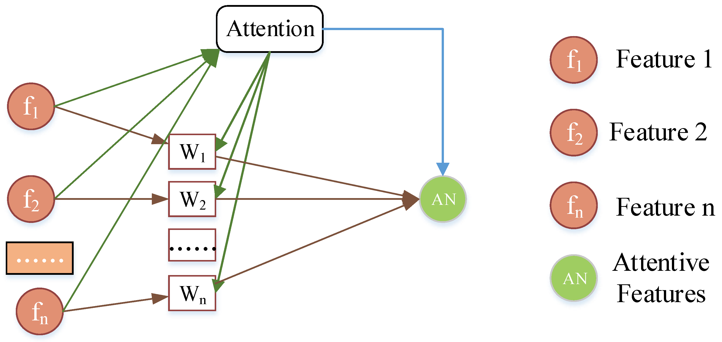
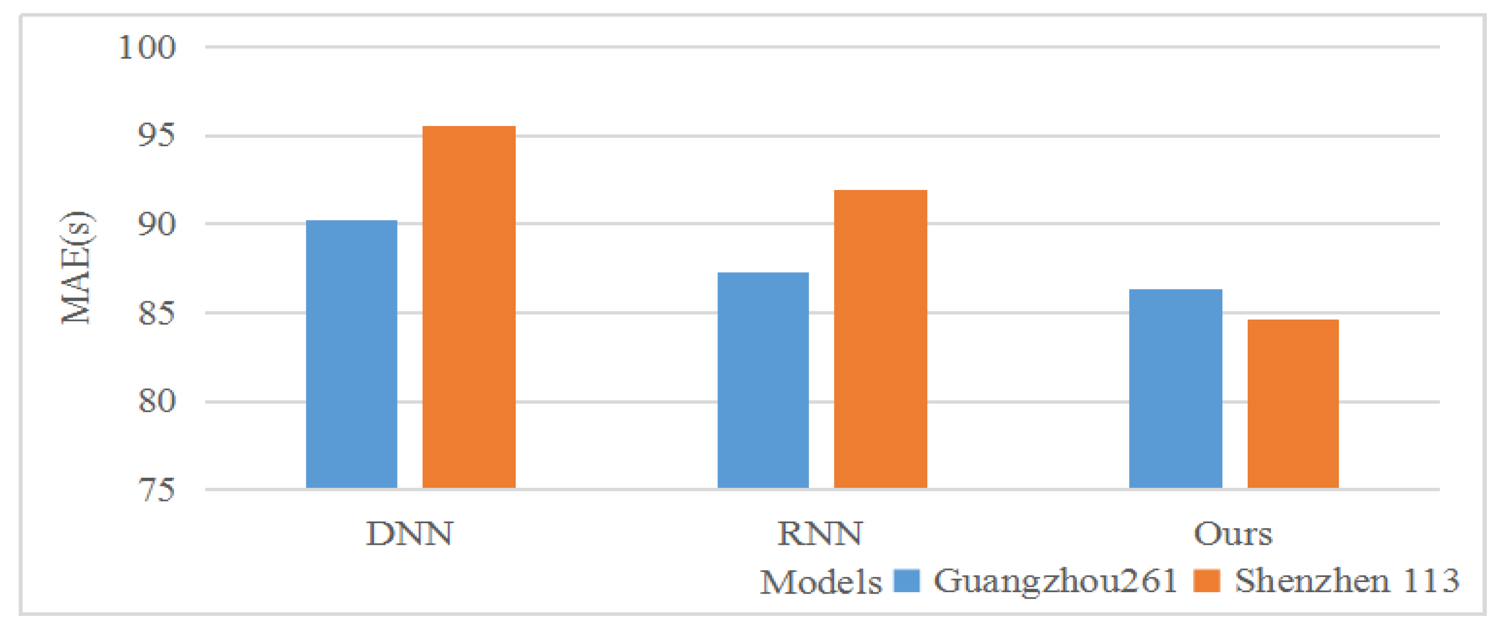
We proposed an embedded network lever WD structure to solve the spatial data and designed an attention mechanism for the RNN to capture the temporal information. Finally, the system used the deep neural network model composed of the RNN and the DNN. The model could capture the non-static spatiotemporal correlation of the urban bus travel time. This enabled the model to generalize the learning model in the cross-temporal and spatial prediction. The model could be used to predict the dynamic travel times of buses. Its effect was better than those of the historical average method, traditional SVR model, SVR-Bayes optimization model, single DNN [5], and RNN [6,21], as shown in Figure 7. The main contributions of this study were as follows.

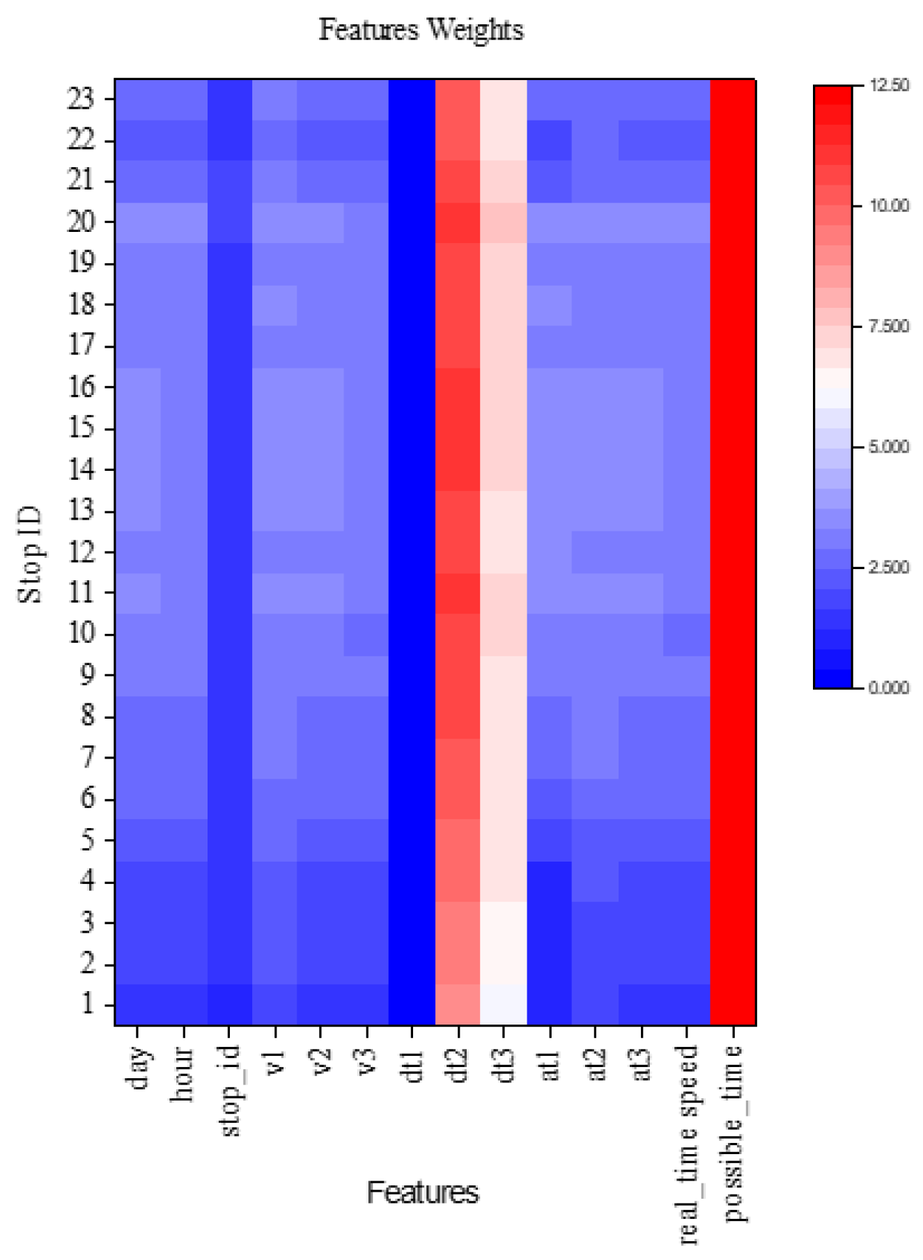
• Based on the prediction of bus travel time, the study proposed a new heterogeneous feature extraction framework based on the RNN model of embedding, WD, and an attention mechanism in order to gain a deep understanding of the space-time features and intrinsic connections of the characteristics related to bus travel time, and to visualize these features and connections, as shown in Table 7 and Table 8, Figure 9.
• Fourteen historical spatial and temporal features were introduced, including the stop IDs as spatial features, bus dwelling times at different historical stages, and real-time GPS bus speeds with real-time possible transit times obtained based on real-time bus speeds as temporal features as shown in Table 2. Especially, the real-time bus speeds is important to improve the dynamic bus travel time prediction, which can be seen in Table 6. These features have not been studied together in previous studies
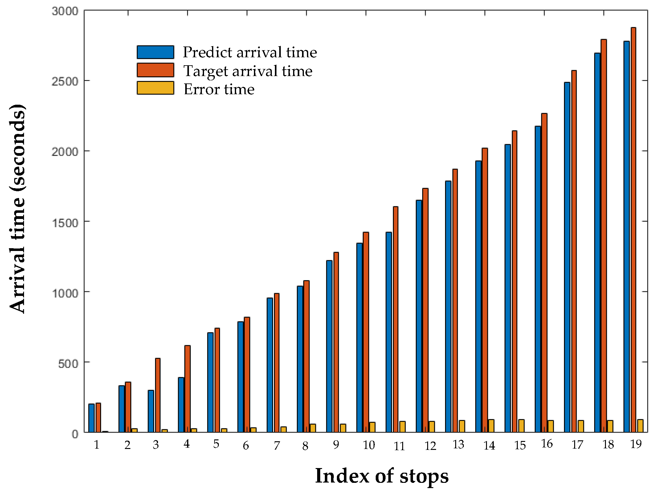
• The multiple super composition of the RNN and DNNs were carried out to reduce the residual heterogeneous data fusion and real-time dynamic bus travel time prediction. A new scheme for real-time dynamic bus travel time prediction was provided as shown in Figure 7 and Figure 8.
• To verify the model’s stability and generalization ability, the model was tested on the data sets of the Guangzhou 226 bus and the Shenzhen 113 bus. The buses ran on the main roads in big cities. Both of the experiments achieved good results. Few of the existing studies tested their models in different cities as shown in Figure 7 and Table 5.

For future work, our study will keep exploring the presented systems in the following directions. In addition to further improving the accuracy of the model, we will extend from one bus line to the bus lines of the entire road network. The existing models tested individual bus routes. The comparison can prove the validity of the model, but our study hold the point that more factors need to be considered. Therefore, it is a feasible choice to try to input the entire road network as a model. With the development of in-deep learning technology, this effect can be achieved through a deep image convolution network of reference image processing [42], which is an important direction of our future research. The effect of missing data on the prediction is obvious. When the missing rate was more than 5%, the performance of the model decreased significantly when only speed was used as the input. When using the multi-attribute fusion, the model had good performance, not only when the error value was low but also when the error growth rate was low, particularly when compared with the model of Liu et al. (2018) [10]. In this research, the missing data were not considered thoroughly enough. In the future, more kinds of sensors (such as ground loops, videos, and geomagnetism) can be considered in order to repair the missing data and to further improve the accuracy.

References

1. Cao, Z.; Ceder, A. Autonomous shuttle bus service timetabling and vehicle scheduling using skip-stop tactic. Transp. Res. Part C Emerg. Technol. 2019, 102, 370–395. [Google Scholar] [CrossRef]
2. Cao, Z.; Ceder, A.; Zhang, S. Real-time schedule adjustments for autonomous public transport vehicles. Transp. Res. Part C Emerg. Technol. 2019, 109, 60–78. [Google Scholar] [CrossRef]
3. Yu, H.; Wu, Z.; Wang, S.; Wang, Y.; Ma, X. Spatiotemporal Recurrent Convolutional Networks for Traffic Prediction in Transportation Networks. Sensors 2017, 17, 1501. [Google Scholar] [CrossRef] [Green Version]
4. Ma, J.; Chan, J.; Ristanoski, G.; Rajasegarar, S.; Leckie, C. Bus travel time prediction with real-time traffic information. Transp. Res. Part C Emerg. Technol. 2019, 105, 536–549. [Google Scholar] [CrossRef]
5. Abdollahi, M.; Khaleghi, T.; Yang, K. An integrated feature learning approach using deep learning for travel time prediction. Expert Syst. Appl. 2020, 139, 112864. [Google Scholar] [CrossRef]
6. He, P.; Jiang, G.; Lam, S.-K.; Sun, Y. Learning heterogeneous traffic patterns for travel time prediction of bus journeys. Inf. Sci. 2020, 512, 1394–1406. [Google Scholar] [CrossRef]
7. Laña, I.; Del Ser, J.; Velez, M.; Vlahogianni, E. Road Traffic Forecasting: Recent Advances and New Challenges. IEEE Intell. Transp. Syst. Mag. 2018, 10, 93–109. [Google Scholar] [CrossRef]
8. Lv, Y.; Duan, Y.; Kang, W.; Li, Z.; Wang, F.-Y. Traffic Flow Prediction With Big Data: A Deep Learning Approach. IEEE Trans. Intell. Transp. Syst. 2014, 16, 1–9. [Google Scholar] [CrossRef]
9. Bengio, Y. Learning Deep Architectures for AI; Now Publishers Inc.: Boston, MA, USA, 2009. [Google Scholar]
10. Liu, Q.; Wang, B.; Zhu, Y. Short-Term Traffic Speed Forecasting Based on Attention Convolutional Neural Network for Arterials. Comput. Civ. Infrastruct. Eng. 2018, 33, 999–1016. [Google Scholar] [CrossRef]
11. Li, L.; Li, Y.; Li, Z. Efficient missing data imputing for traffic flow by considering temporal and spatial dependence. Transp. Res. Part C: Emerg. Technol. 2013, 34, 108–120. [Google Scholar] [CrossRef]
12. Tan, H.; Feng, J.; Feng, G.; Wang, W.; Zhang, Y.-J. Traffic Volume Data Outlier Recovery via Tensor Model. Math. Probl. Eng. 2013, 2013, 1–8. [Google Scholar] [CrossRef]
13. Wu, Y.; Tan, H.; Qin, L.; Ran, B.; Jiang, Z. A hybrid deep learning based traffic flow prediction method and its understanding. Transp. Res. Part C Emerg. Technol. 2018, 90, 166–180. [Google Scholar] [CrossRef]
14. Casas, N. Deep deterministic policy gradient for urban traffic light control. arXiv 2017, arXiv:1703.09035. [Google Scholar]
15. El Hatri, C.; Boumhidi, J. Fuzzy deep learning based urban traffic incident detection. Cogn. Syst. Res. 2018, 50, 206–213. [Google Scholar] [CrossRef]
16. Gu, Y.; Lu, W.; Qin, L.; Li, M.; Shao, Z. Short-term prediction of lane-level traffic speeds: A fusion deep learning model. Transp. Res. Part C Emerg. Technol. 2019, 106, 1–16. [Google Scholar] [CrossRef]
17. Wang, Y.; Zhang, D.; Liu, Y.; Dai, B.; Lee, L.H. Enhancing transportation systems via deep learning: A survey. Transp. Res. Part C Emerg. Technol. 2019, 99, 144–163. [Google Scholar] [CrossRef]
18. Xu, C.; Ji, J.; Liu, P. The station-free sharing bike demand forecasting with a deep learning approach and large-scale datasets. Transp. Res. Part C Emerg. Technol. 2018, 95, 47–60. [Google Scholar] [CrossRef]
19. Tsoi, A.C.; Back, A. Discrete time recurrent neural network architectures: A unifying review. Neurocomputing 1997, 15, 183–223. [Google Scholar] [CrossRef]
20. Li, C.; Wang, J.; Ye, X. Using a Recurrent Neural Network and Restricted Boltzmann Machines for Malicious Traffic Detection. NeuroQuantology 2018, 16, 823–831. [Google Scholar] [CrossRef]
21. Duan, Y.; Lv, Y.; Wang, F.Y. Travel Time Prediction with LSTM Neural Network. In Proceedings of the IEEE 19th International Conference on Intelligent Transportation Systems (ITSC), Rio de Janeiro, Brazil, 1–4 November 2016. [Google Scholar]
22. Petersen, N.C.; Rodrigues, F.; Pereira, F.C. Multi-output bus travel time prediction with convolutional LSTM neural network. Expert Syst. Appl. 2019, 120, 426–435. [Google Scholar] [CrossRef] [Green Version]
23. Xu, H.; Ying, J. Bus arrival time prediction with real-time and historic data. Clust. Comput. 2017, 20, 3099–3106. [Google Scholar] [CrossRef]
24. Liu, Y.; Liu, Z.; Jia, R. DeepPF: A deep learning based architecture for metro passenger flow prediction. Transp. Res. Part C Emerg. Technol. 2019, 101, 18–34. [Google Scholar] [CrossRef]
25. Cheng, H.T.; Koc, L.; Harmsen, J.; Shaked, T.; Shah, H. Wide & Deep Learning for Recommender Systems. In Proceedings of the 1st Workshop on Deep Learning for Recommender Systems, Boston, MA, USA, 15 September 2016. [Google Scholar]
26. Liu, Y.; Wang, Y.; Yang, X.; Zhang, L. Short-term travel time prediction by deep learning: A comparison of different LSTM-DNN models. In Proceedings of the IEEE 20th International Conference on Intelligent Transportation Systems (ITSC), Yokohama, Japan, 16–19 October 2017. [Google Scholar]
27. Oh, S.; Byon, Y.J.; Jang, K.; Yeo, H. Short-term travel-time prediction on highway: A review on model-based approach. KSCE J. Civ. Eng. 2017, 22, 298–310. [Google Scholar] [CrossRef]
28. Cheng, Z.; Chow, M.Y.; Jung, D.; Jeon, J. A big data based deep learning approach for vehicle speed prediction. In Proceedings of the IEEE 26th International Symposium on Industrial Electronics (ISIE), Edinburgh, UK, 19–21 June 2017. [Google Scholar]
29. Ma, Z.; Koutsopoulos, H.N.; Ferreira, L.; Mesbah, M. Estimation of trip travel time distribution using a generalized Markov chain approach. Transp. Res. Part C Emerg. Technol. 2017, 74, 1–21. [Google Scholar] [CrossRef]
30. Kumar, B.A.; Vanajakshi, L.; Subramanian, S. Pattern-based bus travel time prediction under heterogeneous traffc conditions. In Proceedings of the 93rd Annual Meeting—Transportation Research Record, Washington, DC, USA, 12–16 January 2014. [Google Scholar]
31. Watkins, K.E.; Ferris, B.; Borning, A.; Rutherford, G.S.; Layton, D. Where Is My Bus? Impact of mobile real-time information on the perceived and actual wait time of transit riders. Transp. Res. Part A Policy Pr. 2011, 45, 839–848. [Google Scholar] [CrossRef]
32. Chien, S.I.; Ding, Y.; Wei, C. Dynamic Bus Arrival Time Prediction with Artificial Neural Networks. J. Transp. Eng. 2002, 128, 429–438. [Google Scholar] [CrossRef]
33. Rahman, M.; Wirasinghe, S.; Kattan, L. Analysis of bus travel time distributions for varying horizons and real-time applications. Transp. Res. Part C Emerg. Technol. 2018, 86, 453–466. [Google Scholar] [CrossRef]
34. Yang, M.; Chen, C.; Wang, L.; Yan, X.; Zhou, L. Bus arrival time prediction using support vector machine with genetic algorithm. Neural Netw. World 2016, 26, 205–217. [Google Scholar] [CrossRef] [Green Version]
35. Brakewood, C.; Macfarlane, G.S.; Watkins, K. The impact of real-time information on bus ridership in New York City. Transp. Res. Part C Emerg. Technol. 2015, 53, 59–75. [Google Scholar] [CrossRef]
36. Xinghao, S.; Jing, T.; Guojun, C.; QiChong, S. Predicting bus real-time travel time basing on both GPS and RFID data. In Proceedings of the 13th COTA International Conference of Transportation Professionals (CICTP), Shenzhen, China, 13–16 August 2013. [Google Scholar]
37. He, J.; Shen, W.; Divakaruni, P.; Wynter, L.; Lawrence, R. Improving traffic prediction with tweet semantics. In Proceedings of the 23rd International Joint Conference on Artificial Intelligence, Beijing, China, 3–9 August 2013. [Google Scholar]
38. Shalaby, A.; Farhan, A. Prediction Model of Bus Arrival and Departure Times Using AVL and APC Data. J. Public Transp. 2004, 7, 41–61. [Google Scholar] [CrossRef] [Green Version]
39. Zhou, M.; Wang, D.; Li, Q.; Yue, Y.; Tu, W.; Cao, R. Impacts of weather on public transport ridership: Results from mining data from different sources. Transp. Res. Part C Emerg. Technol. 2017, 75, 17–29. [Google Scholar] [CrossRef] [Green Version]
40. Julio, N.; Giesen, R.; Lizana, P. Real-time prediction of bus travel speeds using traffic shockwaves and machine learning algorithms. Res. Transp. Econ. 2016, 59, 250–257. [Google Scholar] [CrossRef]
41. Hans, E.; Chiabaut, N.; Leclercq, L.; Bertini, R.L. Real-time bus route state forecasting using particle filter and mesoscopic modeling. Transp. Res. Part C Emerg. Technol. 2015, 61, 121–140. [Google Scholar] [CrossRef]
42. Zhou, Y.; Yao, L.; Chen, Y.; Gong, Y.; Lai, J. Bus arrival time calculation model based on smart card data. Transp. Res. Part C Emerg. Technol. 2017, 74, 81–96. [Google Scholar] [CrossRef]
Figure 1. Examples of bus and taxi traveling process.
Electronics 09 01876 g001
Figure 2. Embedding extraction of discrete features.
Electronics 09 01876 g002
Figure 3. Illustration of the Wide and Deep model improved based on Cheng et al. (2016) [25].
Electronics 09 01876 g003
Figure 4. Framework of attention model.
Electronics 09 01876 g004
Figure 5. Illustration of the RNN and the attention model.
Electronics 09 01876 g005
Figure 6. Overview of the model developed for the bus dynamic travel time prediction.
Electronics 09 01876 g006
Figure 7. Comparison of different datasets
Electronics 09 01876 g007
Figure 8. Actual/predicted arrival time and cumulative error diagram for each site.
Electronics 09 01876 g008
Figure 9. Average features weighting matrix.
Electronics 09 01876 g009