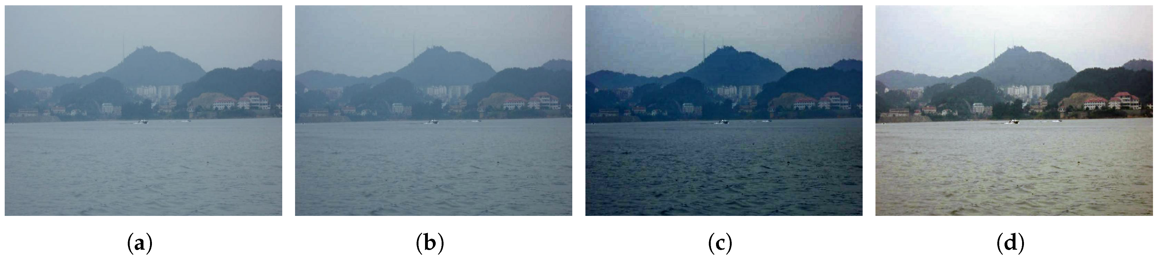
Figure 1.
Overwater image dehazing example. The proposed method generates more clear images compared to state-of-the-art methods. (
a) Hazy input, (
b) Cai [
13], (
c) Yang [
4], (
d) ours.
Figure 1.
Overwater image dehazing example. The proposed method generates more clear images compared to state-of-the-art methods. (
a) Hazy input, (
b) Cai [
13], (
c) Yang [
4], (
d) ours.
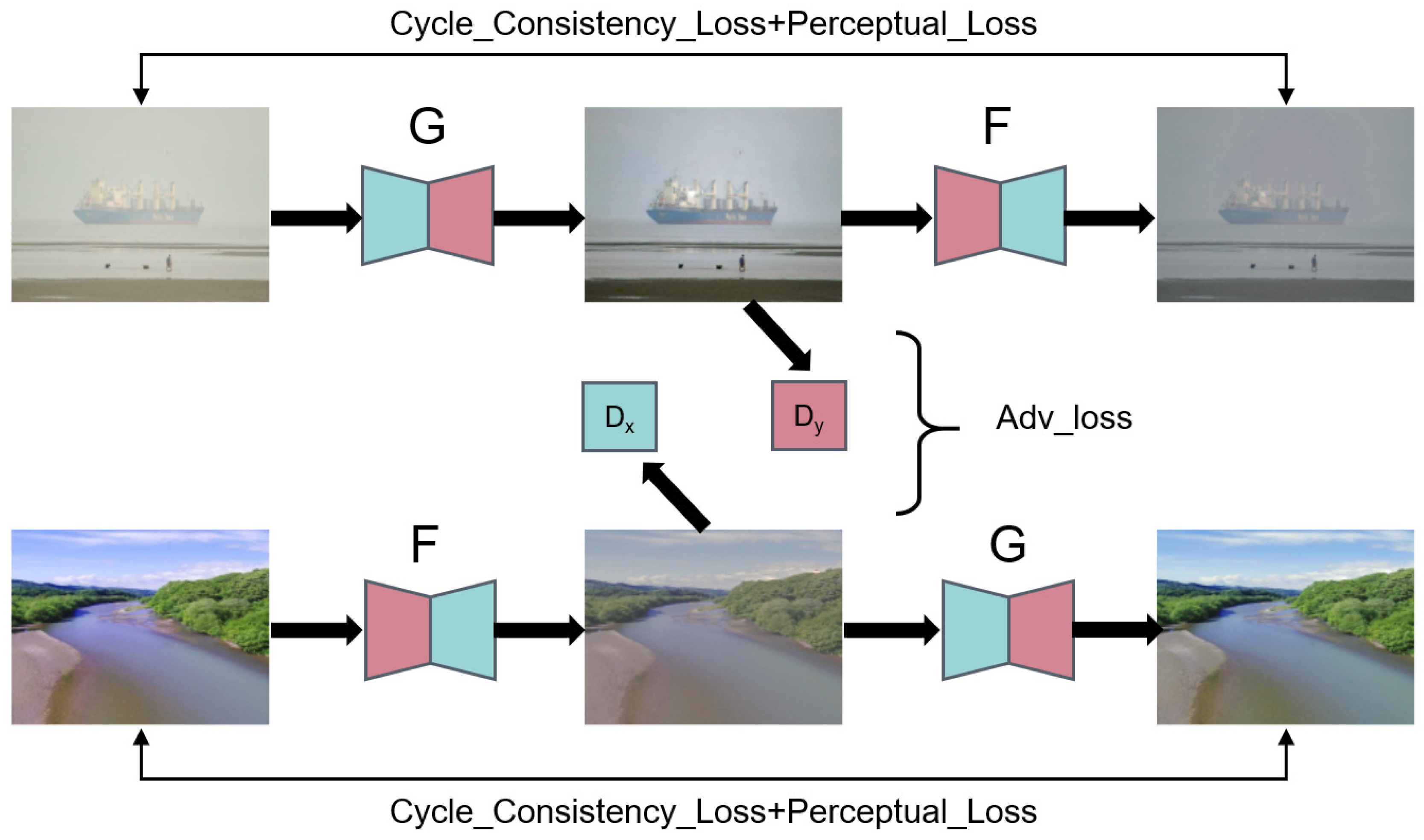
Figure 2.
The main architecture of the proposed OverWater Image (OWI)-Dehazing network. G and F denote generators, where generates clean images from hazy images and vice versa. and denote discriminators. Adversarial loss, cycle consistency loss and perceptual loss are employed to train the network.
Figure 2.
The main architecture of the proposed OverWater Image (OWI)-Dehazing network. G and F denote generators, where generates clean images from hazy images and vice versa. and denote discriminators. Adversarial loss, cycle consistency loss and perceptual loss are employed to train the network.
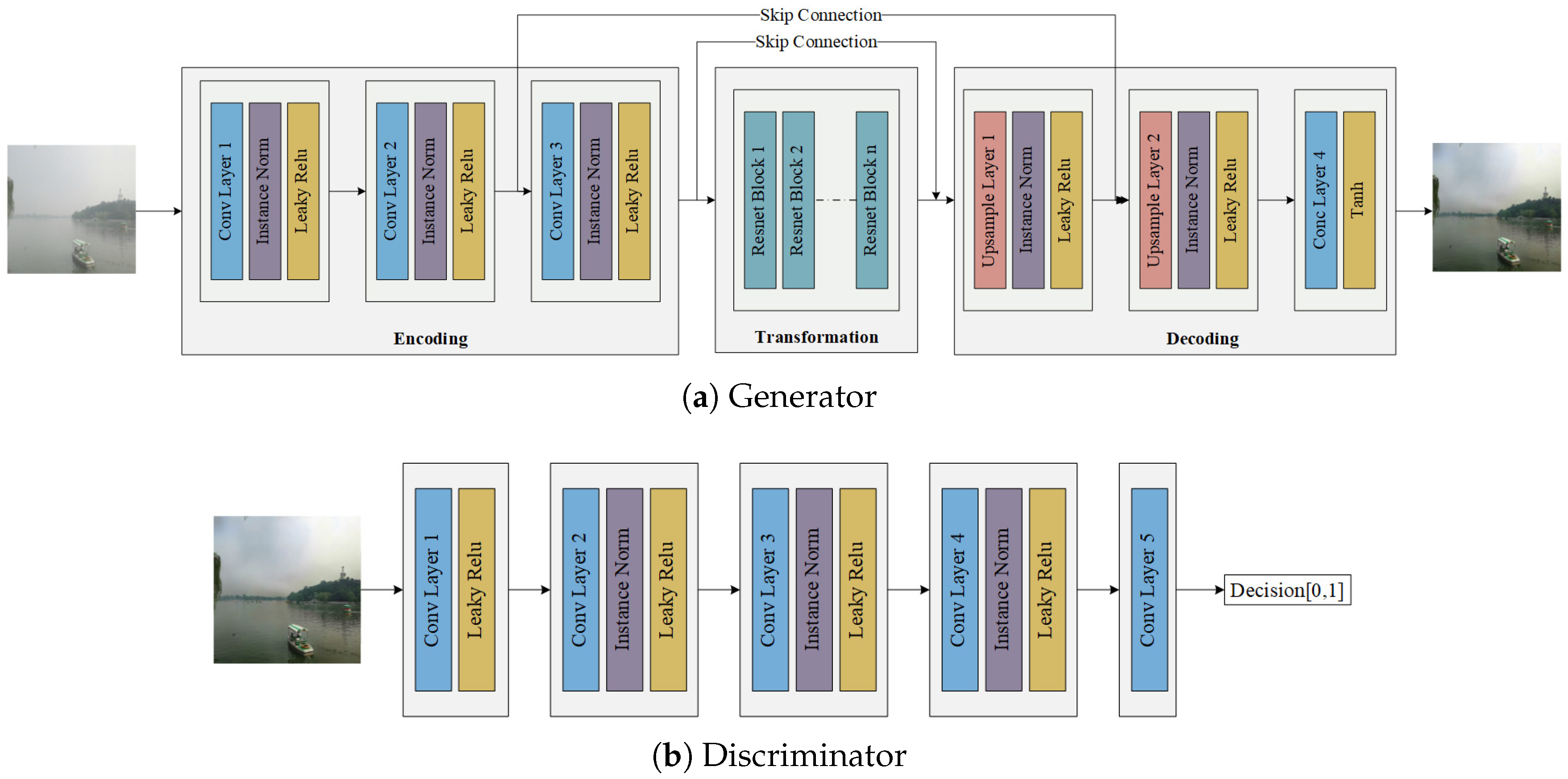
Figure 3.
Architecture of our generator and discriminator. The generator consists of encoding, transformation, and decoding three parts.
Figure 3.
Architecture of our generator and discriminator. The generator consists of encoding, transformation, and decoding three parts.
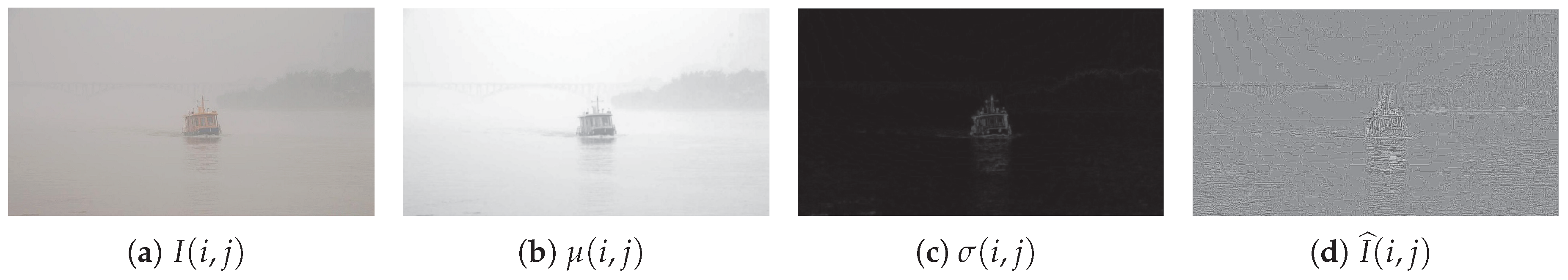
Figure 4.
Examples of mean substracted contrast normalization (MSCN) coefficient.
Figure 4.
Examples of mean substracted contrast normalization (MSCN) coefficient.
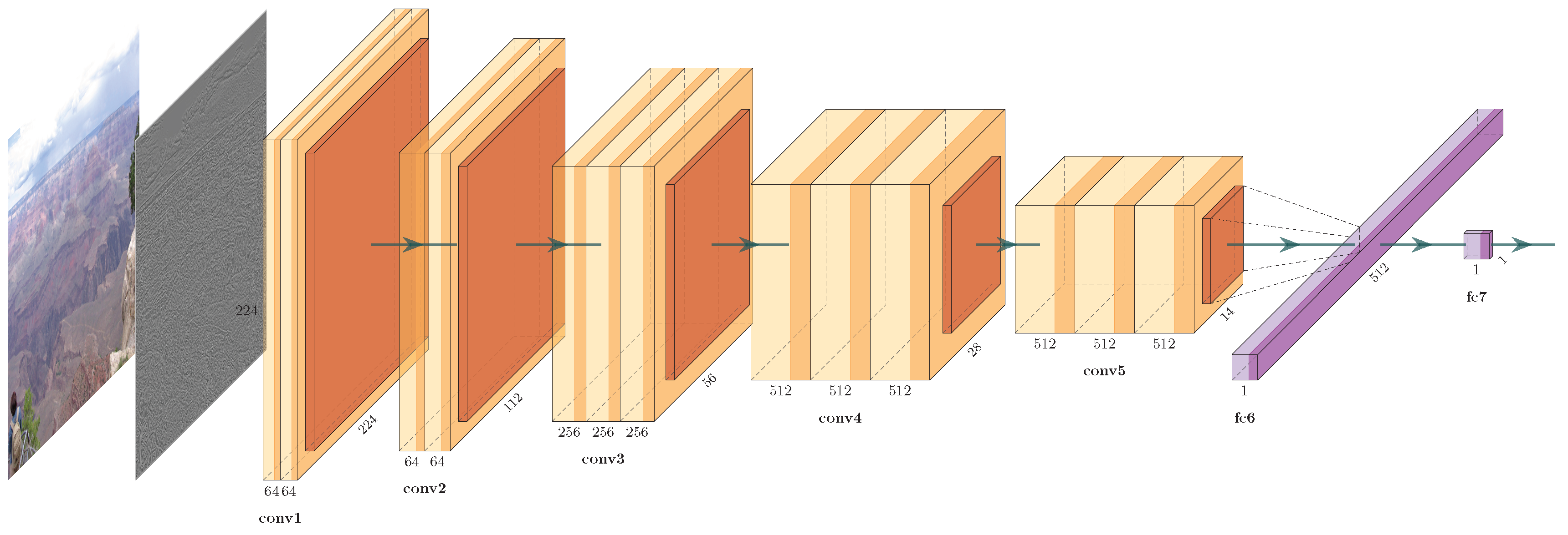
Figure 5.
Architecture of the proposed image quality assessment (IQA) model for dehazed images.
Figure 5.
Architecture of the proposed image quality assessment (IQA) model for dehazed images.
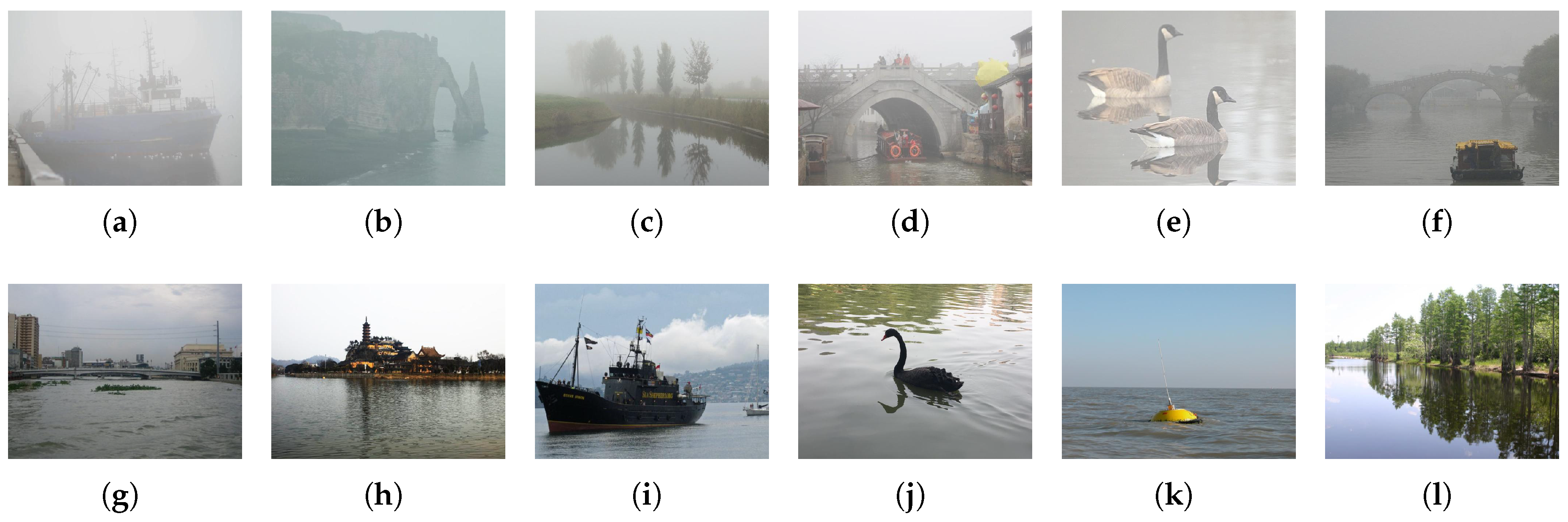
Figure 6.
Examples of HazyWater dataset (best viewed in color). (a–f) Hazy images. (g–l) Clean imags.
Figure 6.
Examples of HazyWater dataset (best viewed in color). (a–f) Hazy images. (g–l) Clean imags.
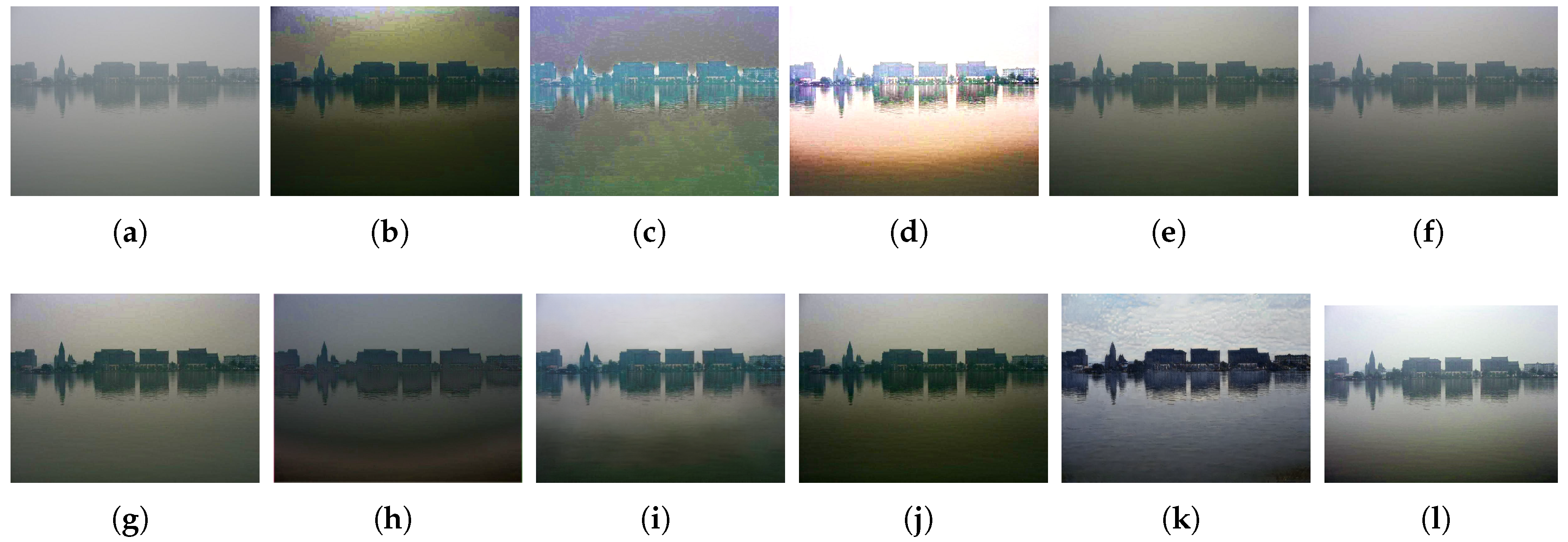
Figure 7.
Real light hazy images and corresponding dehazing results from several state-of-the-art methods (best viewed in color). (a) Hazy Image. (b) DCP. (c) FVR. (d) BCCR. (e) CAP. (f) DehazeNet. (g) MSCNN. (h) AOD-Net. (i) dehaze-cGAN (j) Proximal. (k) CycleGAN. (l) Ours.
Figure 7.
Real light hazy images and corresponding dehazing results from several state-of-the-art methods (best viewed in color). (a) Hazy Image. (b) DCP. (c) FVR. (d) BCCR. (e) CAP. (f) DehazeNet. (g) MSCNN. (h) AOD-Net. (i) dehaze-cGAN (j) Proximal. (k) CycleGAN. (l) Ours.
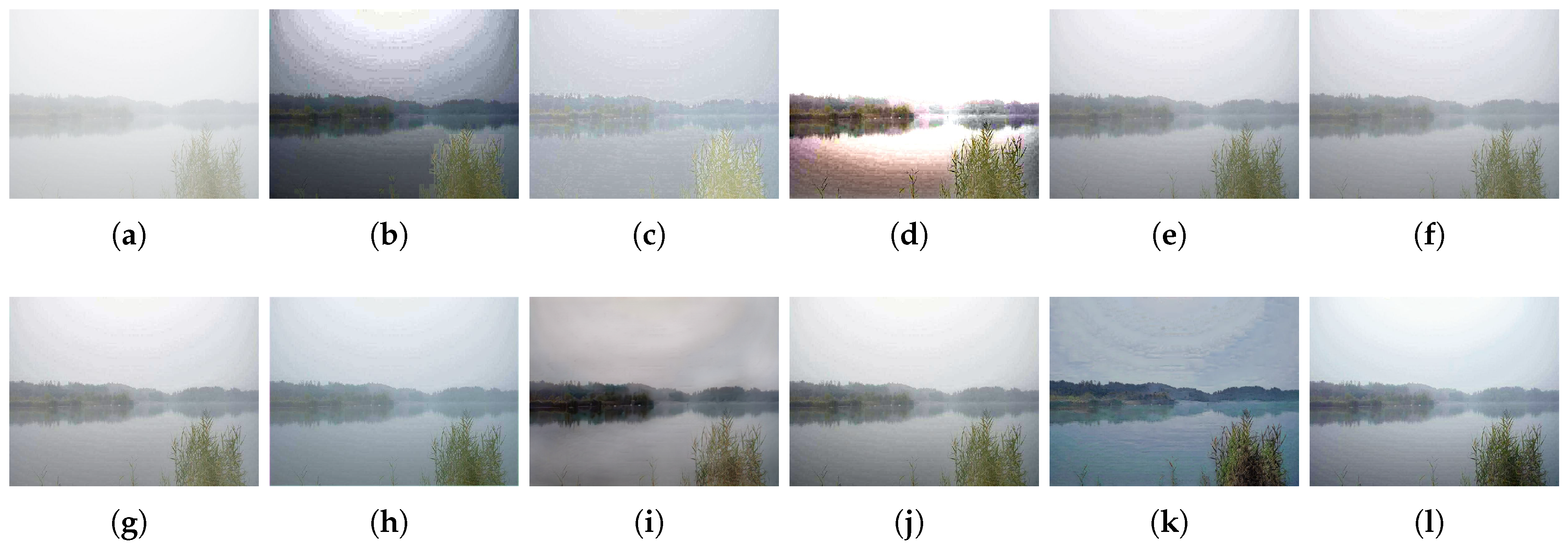
Figure 8.
Real heavy hazy images and corresponding dehazing results from several state-of-the-art methods (best viewed in color). (a) Hazy Image. (b) Dark-channel prior (DCP). (c) FVR. (d) BCCR. (e) Color attenuation prior (CAP). (f) DehazeNet. (g) MSCNN. (h) AOD-Net. (i) dehaze-cGAN (j) Proximal. (k) CycleGAN. (l) Ours.
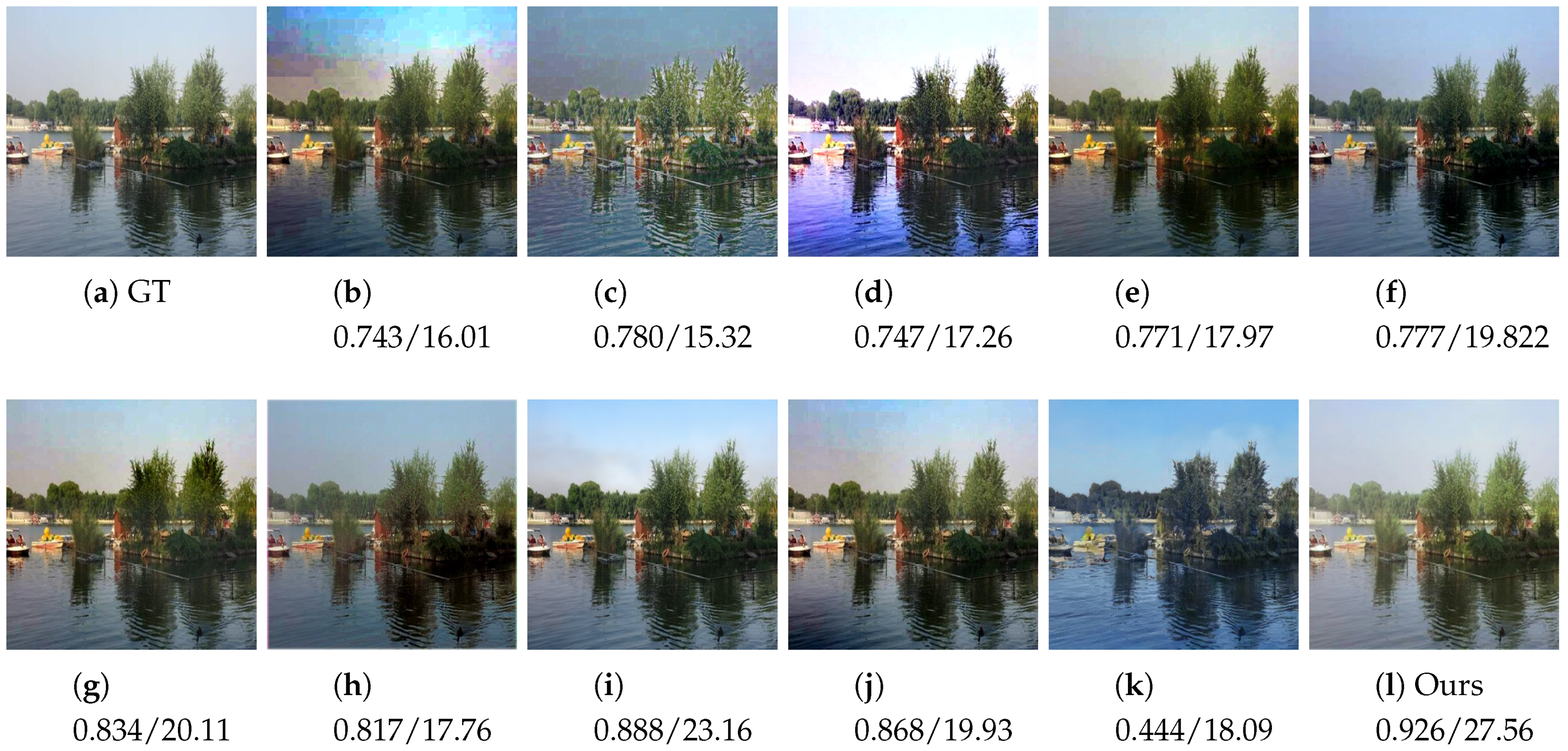
Figure 9.
Comparison in terms of SSIM/PSNR for different image dehazing methods. (a) Ground Truth. (b) DCP. (c) FVR. (d) BCCR. (e) CAP. (f) DehazeNet. (g) MSCNN. (h) AOD-Net. (i) dehaze-cGAN. (j) Proximal. (k) CycleGAN. (l) Ours.
Figure 9.
Comparison in terms of SSIM/PSNR for different image dehazing methods. (a) Ground Truth. (b) DCP. (c) FVR. (d) BCCR. (e) CAP. (f) DehazeNet. (g) MSCNN. (h) AOD-Net. (i) dehaze-cGAN. (j) Proximal. (k) CycleGAN. (l) Ours.
Figure 10.
Examples of paired data generated by our network. (a–d) Clean images. (e–h) Generated hazy images corresponding to (a–d).
Figure 10.
Examples of paired data generated by our network. (a–d) Clean images. (e–h) Generated hazy images corresponding to (a–d).
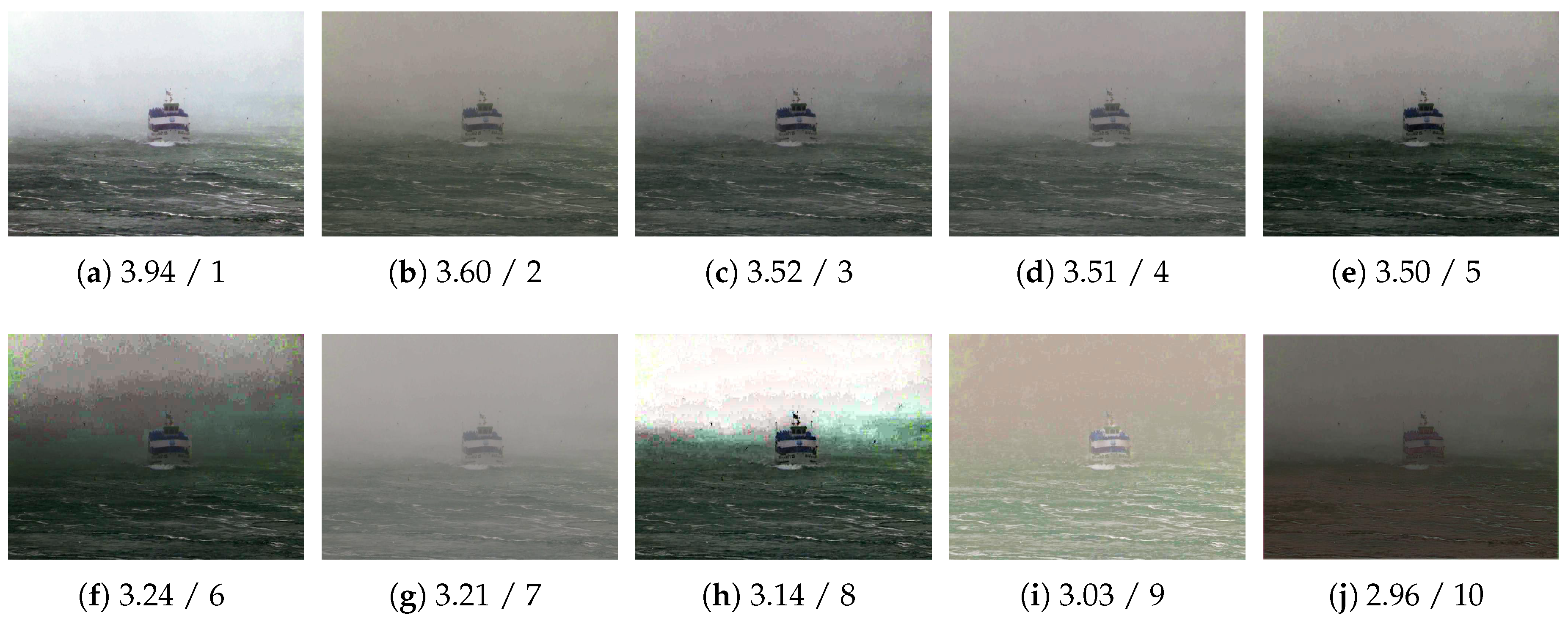
Figure 11.
Comparison via the proposed IQA model. Ranking scores and the rankings are shown below each image. (a) Ours. (b) CAP. (c) MSCNN. (d) DehazeNet. (e) Proximal. (f) DCP. (g) Input. (h) BCCR. (i) FVR. (j) AOD-Net.
Figure 11.
Comparison via the proposed IQA model. Ranking scores and the rankings are shown below each image. (a) Ours. (b) CAP. (c) MSCNN. (d) DehazeNet. (e) Proximal. (f) DCP. (g) Input. (h) BCCR. (i) FVR. (j) AOD-Net.
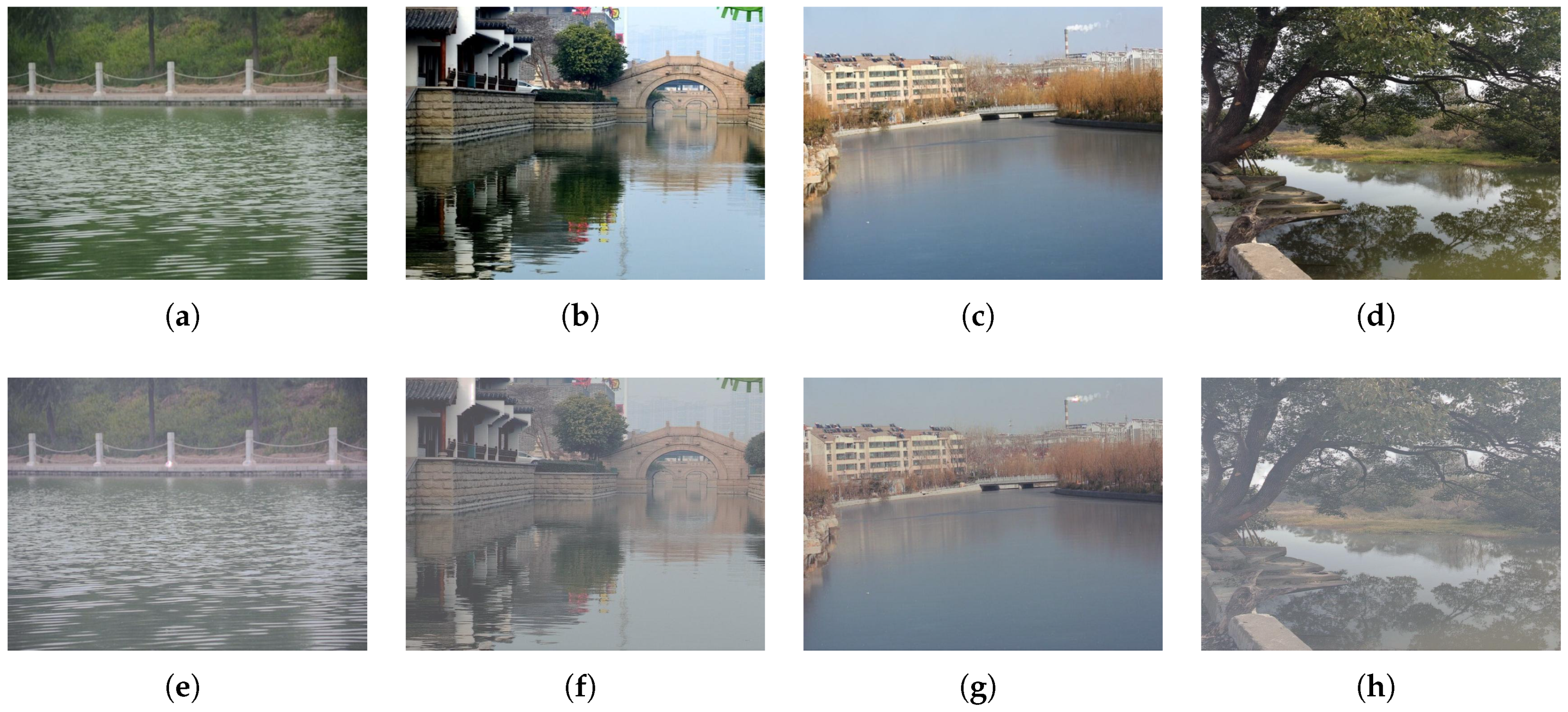
Figure 12.
Examples of color cast. (a,f) Two hazy images. (b,g) Generated by DCP. (c,h) Generated by DehazeNet. (d,i) Generated by MSCNN. (e,j) Our results. Compared with DCP, DehazeNet and MSCNN, our method effectively corrects the color cast phenomenon and produces a visual better image.
Figure 12.
Examples of color cast. (a,f) Two hazy images. (b,g) Generated by DCP. (c,h) Generated by DehazeNet. (d,i) Generated by MSCNN. (e,j) Our results. Compared with DCP, DehazeNet and MSCNN, our method effectively corrects the color cast phenomenon and produces a visual better image.
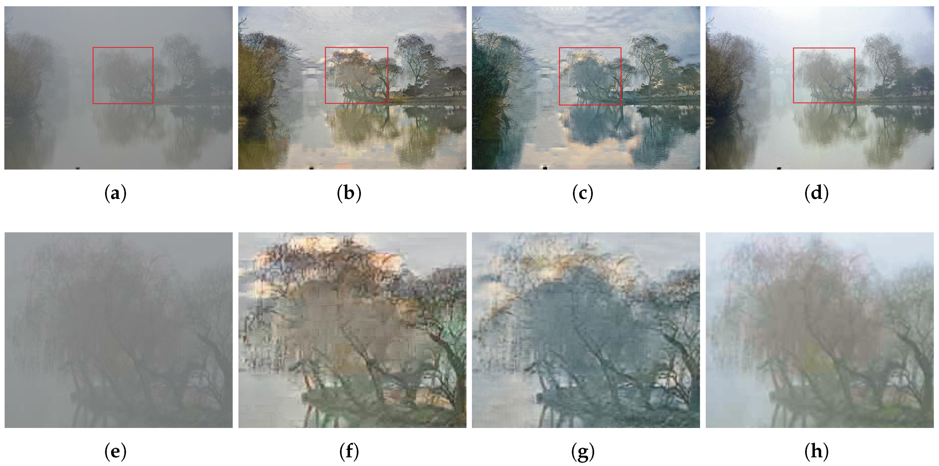
Figure 13.
Effectiveness of the proposed network with resize convolution. (a,e) Input hazy images. (b,f) Dehazed images using deconvolution. (c,g) The dehazed images using sub-pixel convolution. (d,h) Denote dehazed results using resize convolution (ours). (e–h) The zoom-in views of (a–d), separately.
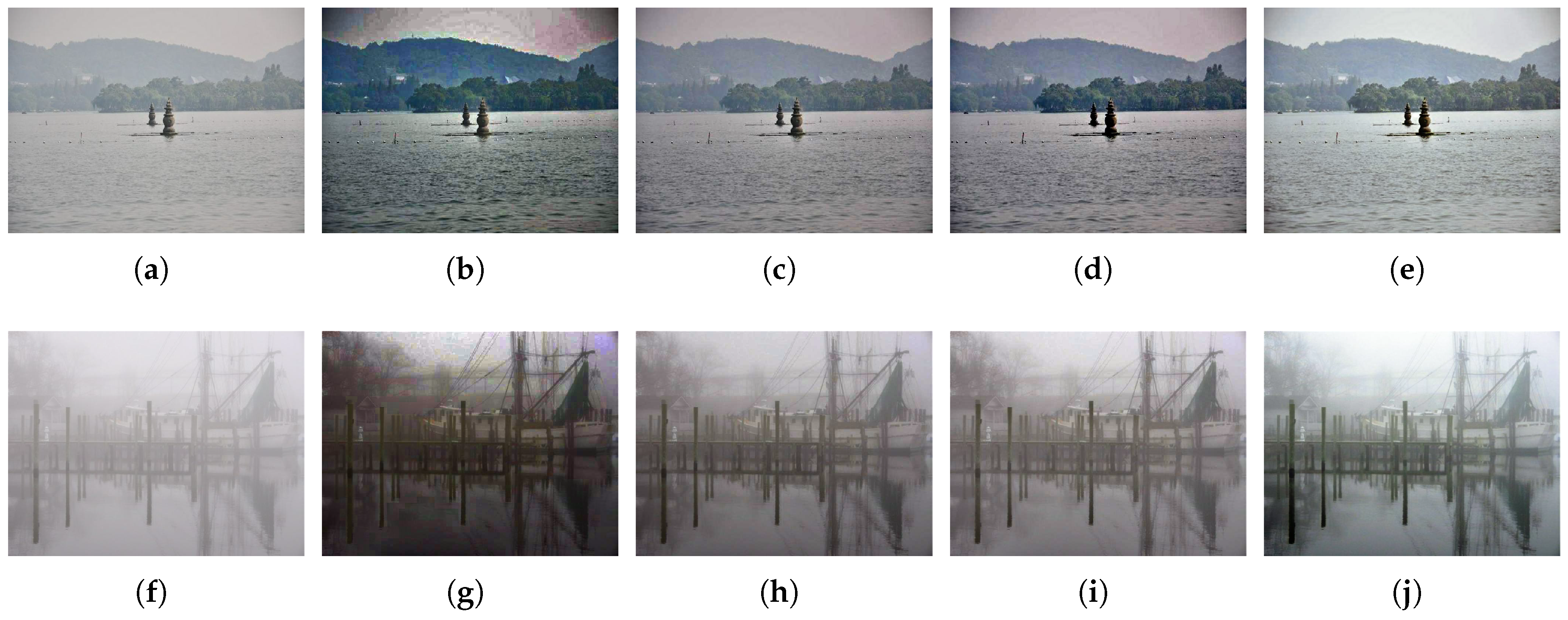
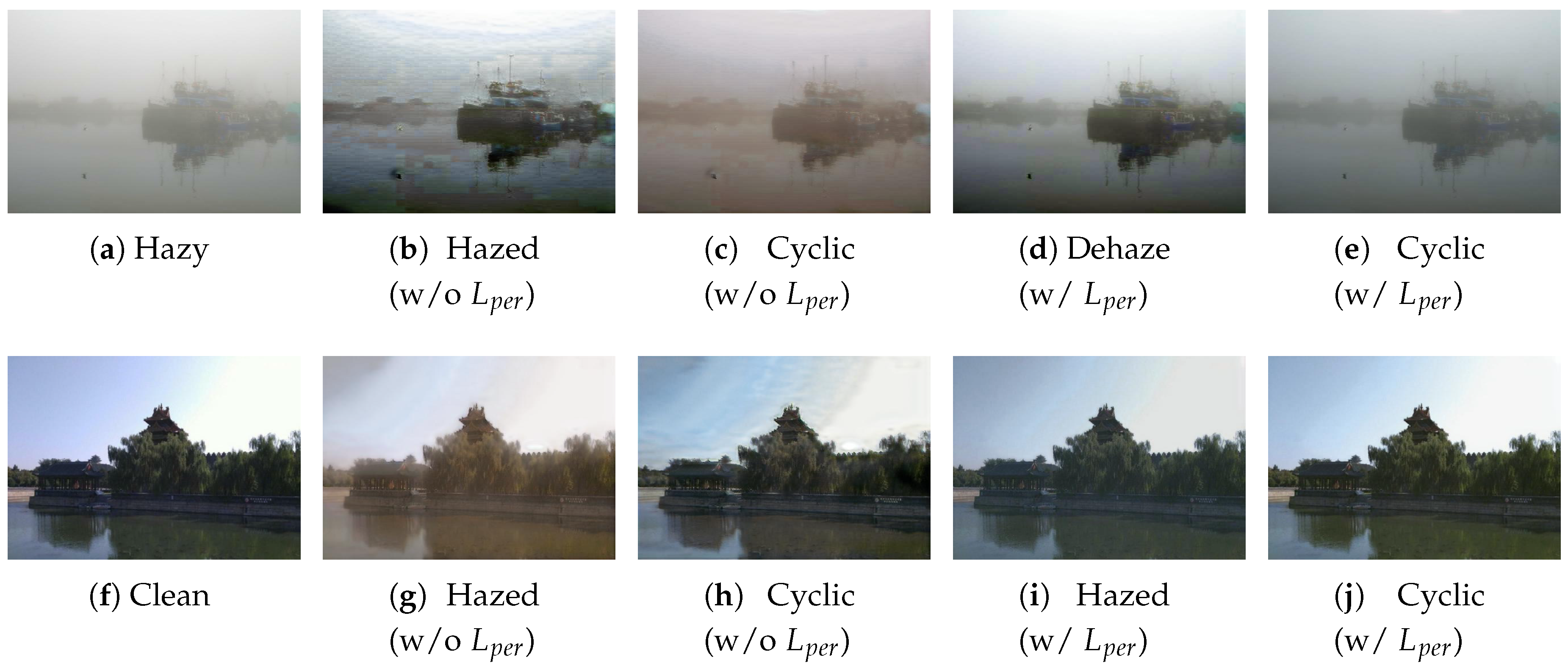
Figure 14.
Comparison of dehazing with and without perceptual loss. (a–e) The generation direction of . (f–j) The direction of formation is . “(w/o )” denotes the network without perceptual loss, and “(w/ )” denotes the network with perceptual loss.
Figure 14.
Comparison of dehazing with and without perceptual loss. (a–e) The generation direction of . (f–j) The direction of formation is . “(w/o )” denotes the network without perceptual loss, and “(w/ )” denotes the network with perceptual loss.
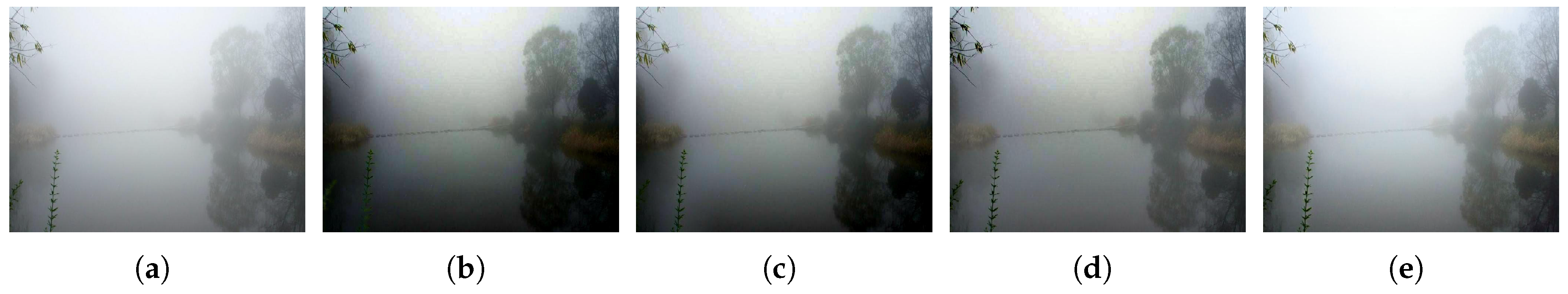
Figure 15.
Example of failure cases. (a) Input image. (b) CAP. (c) DehazeNet. (d) MSCNN. (e) Ours.
Figure 15.
Example of failure cases. (a) Input image. (b) CAP. (c) DehazeNet. (d) MSCNN. (e) Ours.
Table 1.
Main parameters of our generator. ‘#In’ denotes the number of input channel, and ‘#Out’ represents the number of output channel. ‘Upsample’ denotes the resize convolution.
Table 1.
Main parameters of our generator. ‘#In’ denotes the number of input channel, and ‘#Out’ represents the number of output channel. ‘Upsample’ denotes the resize convolution.
| Layer Name | #In | #Out | Kernel | Strides |
|---|
| Conv 1 | 3 | 32 | | 1 |
| Conv 2 | 32 | 64 | | 2 |
| Conv 3 | 64 | 128 | | 2 |
| Res Block 1 | 128 | 138 | | 1 |
| ... | ... | ... | ... | ... |
| Res Block 9 | 128 | 128 | | 1 |
| Upsample 1 | 256 | 64 | | 2 |
| Upsample 2 | 128 | 32 | | 2 |
| Conv 4 | 32 | 3 | | 1 |
| Tanh | - | - | - | - |
Table 2.
Main parameters of our discriminator. ‘#In’ denotes the number of input channel, and ‘#Out’ represents the number of output channel.
Table 2.
Main parameters of our discriminator. ‘#In’ denotes the number of input channel, and ‘#Out’ represents the number of output channel.
| Layer Name | #In | #Out | Kernel | Strides |
|---|
| Conv 1 | 3 | 32 | | 2 |
| Conv 2 | 32 | 64 | | 2 |
| Conv 3 | 64 | 128 | | 2 |
| Conv 4 | 128 | 256 | | 2 |
| Conv 5 | 256 | 1 | | 1 |
Table 3.
Average PSNR, SSIM, and CIEDE2000 values of dehazed results on the new synthetic dataset. The best result, the second result, and the third place result are represented by red, blue, and green, respectively. The average values of PSNR, SSIM and CIEDE2000 results calculated directly between the each hazy and its corresponding clean image.
| | FVR | DCP | BCCR | CAP | DehazeNet | MSCNN | AOD-Net | Proximal | dehaze-cGAN | CycleGAN | Ours |
|---|
| SSIM | 0.817 | 0.717 | 0.680 | 0.825 | 0.867 | 0.850 | 0.835 | 0.820 | 0.876 | 0.584 | 0.893 |
| PSNR | 16.56 | 14.57 | 13.92 | 19.50 | 23.27 | 20.55 | 19.33 | 17.79 | 22.77 | 18.31 | 24.93 |
| CIEDE2000 | 11.71 | 14.92 | 15.35 | 9.37 | 6.23 | 7.81 | 9.11 | 10.14 | 6.51 | 11.5 | 5.98 |
Table 4.
Comparison of dehazed image quality using four image quality assessment methods. The top three results are in red, blue, and green font, respectively.
Table 4.
Comparison of dehazed image quality using four image quality assessment methods. The top three results are in red, blue, and green font, respectively.
| | FADE [48] ↓ | SSEQ [54] ↓ | BLINDS-2 [55] ↓ | NIMA [56] ↑ |
|---|
| Ours | 1.95 | 36.24 | 31.50 | 6.47 |
| CAP | 3.03 | 40.97 | 51.00 | 5.95 |
| MSCNN | 2.38 | 45.56 | 50.50 | 6.23 |
| DehazeNet | 3.11 | 42.49 | 49.50 | 6.12 |
| Proximal-Dehaze | 1.69 | 43.69 | 54.50 | 6.06 |
| DCP | 1.45 | 43.32 | 51.50 | 5.36 |
| BCCR | 1.17 | 45.76 | 48.50 | 6.08 |
| FVR | 2.67 | 41.71 | 48.00 | 4.86 |
| AOD-Net | 2.30 | 38.62 | 54.50 | 6.15 |
Table 5.
Average run time (in seconds) on synthetic data. The top three results are highlighted in red, blue, and green font, respectively.
Table 5.
Average run time (in seconds) on synthetic data. The top three results are highlighted in red, blue, and green font, respectively.
| Methods | Time () | Run Environment |
|---|
| DCP | 15.55 | Matlab |
| FVR | 3.87 | Matlab |
| CAP | 0.94 | Matlab |
| DehazeNet | 1.02 | Matlab |
| MSCNN | 1.97 | Matlab |
| AOD-Net | 0.23 | PyTorch |
| dehaze-cGAN | 0.64 | Torch7 |
| Ours | 0.30 | TensorFlow |
Table 6.
Average scores in terms of PSNR, SSIM, and CIEDE2000 for deconvolution, sub-pixel convolution, and resize convolution on the synthetic test set from HazyWater Dataset.
Table 6.
Average scores in terms of PSNR, SSIM, and CIEDE2000 for deconvolution, sub-pixel convolution, and resize convolution on the synthetic test set from HazyWater Dataset.
| Average Metrics | SSIM | PSNR | CIEDE2000 |
|---|
| Deconvolution | 0.758 | 20.34 | 9.12 |
| Sub-pixel Convolution | 0.643 | 20.21 | 10.86 |
| Resize Convolution | 0.819 | 22.19 | 7.41 |
Table 7.
Effect of perceptual loss in terms of SSIM, PSNR, and CIEDE2000. CycleGAN loss refers to the formulation of adversarial loss and cycle consistency loss, VGG loss refers to substitute perceptual loss.
Table 7.
Effect of perceptual loss in terms of SSIM, PSNR, and CIEDE2000. CycleGAN loss refers to the formulation of adversarial loss and cycle consistency loss, VGG loss refers to substitute perceptual loss.
| Average Metrics | SSIM | PSNR | CIEDE2000 |
|---|
| CycleGAN loss | 0.819 | 22.19 | 7.41 |
| CycleGAN loss + VGG loss | 0.893 | 24.93 | 5.98 |


