Backstepping Fuzzy Sliding Mode Control for the Antiskid Braking System of Unmanned Aerial Vehicles

Abstract

This paper proposes a backstepping fuzzy sliding mode control method for the antiskid braking system (ABS) of unmanned aerial vehicles (UAVs). First, the longitudinal dynamic model of the UAV braking system is established and combined with the model of the electromechanical actuator (EMA), based on reasonable simplification. Subsequently, to overcome the higher-order nonlinearity of the braking system and ensure the lateral stability of the UAV during the braking process, an ABS controller is designed using the barrier Lyapunov function to ensure that the slip ratio can track the reference value without exceeding the preset range. Then, a power fast terminal sliding mode control algorithm is adopted to realize high-performance braking pressure control, which is required in the ABS controller, and a fuzzy corrector is established to improve the dynamic adaptation of the EMA controller in different braking pressure ranges. The experimental results show that the proposed braking pressure control strategy can improve the servo performance of the EMA, and the hardware in loop (HIL) experimental results indicate that the proposed slip ratio control strategy demonstrates a satisfactory performance in terms of stability under various runway conditions.

1. Introduction

With the development of unmanned aerial vehicle (UAV) technology, the safe recycling of UAVs has been drawing increasing research attention. The braking system plays a pivotal role during the takeoff and landing processes, which are crucial to ensure the safe recycling of UAV. As the size and weight of the newly developed UAVs have been increasing fast, the performance of the braking system is becoming increasingly important [1,2,3]. Most of the aircraft braking systems use a hydraulic system as the power source, for which long hydraulic lines are required, and this means the hydraulic braking system has a considerable influence on the structure of the UAV [4,5,6]. In addition, the risk of oil leakage in the hydraulic system cannot be ignored. The electromechanical actuator (EMA) is a new type of actuator, which is composed of a brushless DC motor (BLDCM), a reduction gear, a ball screw and a controller. It has the advantages of a small size, a light weight and a high reliability [7,8]. By using the EMA in the UAV braking system, the braking efficiency and safety can be enhanced [9,10].

The dynamic performance of the UAV braking system depends on not only the actuating mechanism but also the advanced braking control strategy. Typically, the use of sensors is very common in autonomous robotics systems (e.g., mobile robots [11] and inspection robotic arms [12]) for purposes such as collision avoidance and testing, and therefore equipping the UAV with sensors is mandatory as a kind of aerial robot. By using various sensors, such as the acceleration sensor, the velocity and acceleration of the UAV can be obtained, which makes it easier to apply an advanced antiskid control strategy in the UAV braking system. Certain control systems use the slip velocity to control the braking pressure of the aircraft. However, the limitations of poor efficiency and unsteadiness limit the control effects of such control systems. With continued innovations in control theory, the slip ratio control has been regarded as a better antiskid control strategy. The main concept of the slip ratio control involves attempting to maintain the actual slip ratio at its optimal value, which results in the maximum adhesive coefficient between the wheel and runway. According to the relationship between the slip ratio and the adhesive coefficient, if the actual slip ratio considerably exceeds the optimal value, the wheel may skid out of control, and this will reduce the lateral stability of the UAV. Therefore, it is important to maintain the stability of the slip ratio.

In the existing literature on the ABS controller, several slip ratio control strategies have been proposed, such as fuzzy control [13], sliding mode control [14] and neural network control [15]. A hybrid ABS control algorithm using force measurement was proposed in [16] by Corno et al., and a two-phase slip ratio control method was presented. Seibum et al. developed a new type of antilock braking system control strategy in [17], and a feedback control method was adopted to differentiate the ABS controller from the traditional algorithms. In [18,19], several novel slip ratio control methods were proposed, and the response speeds of the ABS controller were improved significantly. However, the slip ratio is regarded as a simple control object in the above studies, while its maximum value is not constrained. There are few studies that have been focused on the lateral stability control of the braking system in aircraft, which makes these control strategies difficult to be applied in practice. Thus, it is necessary to select an appropriate slip ratio control algorithm in the ABS controller, as there is high order nonlinearity in the braking system of aircrafts. Meanwhile, the maximum value of the slip ratio must be limited, which can ensure the lateral stability of aircrafts during the braking process.

Before establishing the ABS controller, an appropriate dynamic mathematical model of the UAV is necessary. The actual mathematical model of a UAV is highly complicated—the kinetic equations of 6 degrees of freedom (DOF) have been defined in [20], and the interaction between the landing gear and antiskid braking system was clarified in [21]. In fact, a complex UAV mathematical model is not conducive for the design of the slip ratio control strategy. A rational simplified mathematical model of the UAV is the basis of the ABS controller, and the aerodynamic effects on the UAV also need to be considered [22].

The final actuator of the electric braking system is an EMA, so it is important for the EMA controller to demonstrate a satisfactory braking pressure control performance. The EMA is a complex nonlinear system, and the large fluctuations in temperature during the braking process can considerably change the parameters of the BLDCM. These characteristics make it difficult to achieve a fast response and high precision when using a traditional linear controller. Therefore, it is necessary to develop a nonlinear EMA controller to realize the braking pressure control requirements of the ABS controller. Several different motor control algorithms were proposed by Mercorelli in [23] and [24]. With the objective of improving the system response speed, Wu et al., in [25], proposed a nonlinear sliding mode surface with terminal characteristics, but there are few studies about the EMA controller in electric braking systems.

In order to realize the high-performance control of the UAV braking system, a rational and simplified dynamic mathematical model of the UAV is established. Then, the controller of the UAV braking system is divided into two parts: the ABS controller and the EMA controller. A logarithmic barrier Lyapunov function is proposed to constrain the slip ratio value of the UAV in the ABS controller. By using the power fast terminal sliding mode algorithm, the electromagnetic torque control law of the EMA can be derived from the backstepping design principle. To ensure that the EMA controller has adaptive capability under different braking pressure ranges, a fuzzy corrector is built to adjust the control parameters of the sliding mode controller in real-time. Compared with the routine control strategies, the proposed ABS controller can constrain the slip ratio and maintain the working point around the optimal value, and the EMA controller also has a better braking pressure control effect. As a result, the lateral stability of the UAV braking system is improved significantly.

The rest of paper is organized as follows: Section 2 describes the mathematical model of the antiskid braking system, and the UAV mathematical model and the EMA mathematical model are established in order; furthermore, the corresponding control objectives are defined. Section 3 presents the design method of the backstepping-based ABS controller and the fuzzy sliding mode EMA controller. Section 4 discusses the results of the used hardware in loop experiments. The conclusions are summarized in Section 5.

2. Mathematical Model of Antiskid Braking System for UAV

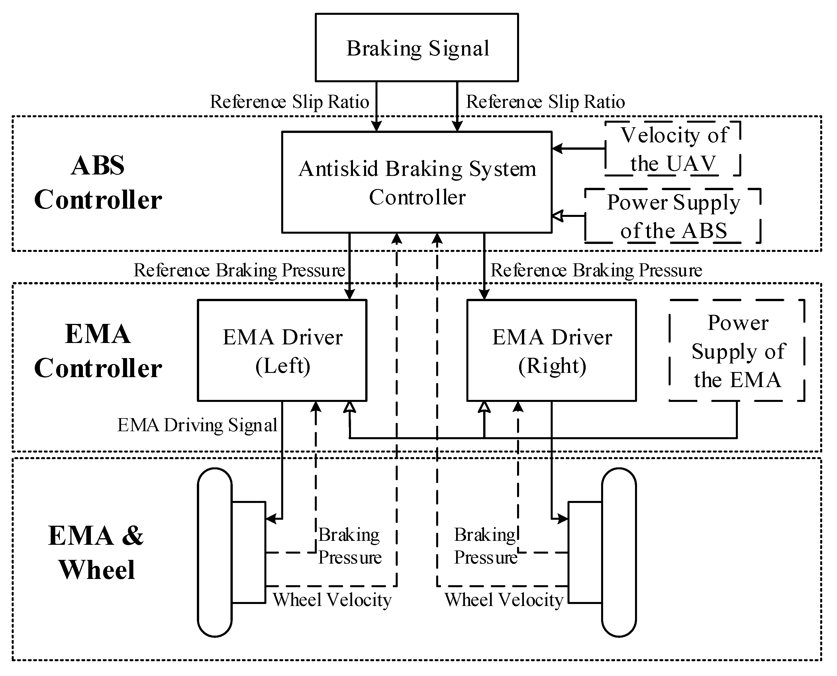
There are three basic classes of mathematical models: empirical, optimization and structural. The mathematical model of the UAV antiskid braking system in this paper is developed based on the structural model, and the control structure is shown in Figure 1. There are three parts of the UAV antiskid braking system: the ABS controller, the EMA controller and the EMA. The ABS controller is used to control the slip ratio and output the reference braking pressure signal, then the EMA controller takes the received reference braking pressure as the control target and outputs the EMA driving signal. Finally, the EMA implements the corresponding braking actions.

Prior to the model analysis, the following assumptions must be defined: (1) The UAV is assumed to be an ideal rigid body, and the weight of the UAV is centered on a mass point. (2) The lateral motion is neglected, and only the longitudinal motion is considered. (3) The braking performance of the wheels on both sides is identical, and the tire compression is ignored.

2.1. UAV Mathematical Model

The force analysis during the braking process of the UAV is shown in Figure 2:

where $V_x$ is the longitudinal velocity, $F_L$ is the lift force, $T$ is the residual thrust of the engine, $F_x$ is the aerodynamic drag, $m$ is the weight of the UAV, $F_f$ and $F_b$ are the friction forces between the wheel and the runway, $N_f$ and $N_b$ are the support forces between the wheel and the runway, $a$ is the distance between the front wheel and center of gravity of the UAV, $b$ is the distance between the back wheel and center of gravity of the UAV, and $h$ is the distance between the center of gravity of the UAV and the runway.

The longitudinal motion equation, vertical force balance equation and torque balance equation can be generated as

$$\{\begin{array}{l}m\stackrel{·}{V_x}+F_f+n{F}_b+F_x-T=0\\ F_L+N_f+n{N}_b-mg=0\\ N_{f}a-n{N}_{b}b-(F_f+n{F}_b)h=0\end{array}$$

(1)

where $n$ is the number of back wheels.

The lift force, $F_L$, and aerodynamic drag, $F_x$, can be generated as

$$F_L=0.5C_L{\rho }_a{S}_L{V}_x^2,F_x=0.5C_P{\rho }_a{S}_P{V}_x^2$$

(2)

where $C_L$ is the lift coefficient, ${\rho }_a$ is the air density, $S_L$ is the aerodynamic lift area, $C_P$ is the aerodynamic drag coefficient, and $S_P$ is the aerodynamic drag area.

The braking pressure is usually applied to the back wheel [26], and the dynamic equation of the back wheel can be expressed as

$$F_{b}r-T_b-B_w\omega =\dot{\omega }{I}_w$$

(3)

where $r$ is the radius of the back wheel, $T_b$ is the braking torque, $B_w$ is the axle friction factor, $\omega$ is the angular velocity of the back wheel, and $I_w$ is the moment of inertia of the back wheel.

If the nonlinear factors, such as the change in the shape of the brake disc, vibration and tire wear, are neglected [27], the braking torque, $T_b$, can be calculated using the braking pressure, $p$:

$$T_b=k_{b}p$$

(4)

where $k_b$ is the braking torque conversion factor.

2.2. Slip Ratio Model

When a UAV lands on the runway, the braking pressure, $p$, is applied to the back wheels, and the longitudinal velocity of the UAV is larger than the velocity of the back wheels [28]. Then the slip ratio, $\lambda$, can be defined as

$$\lambda =\left(V_x-\omega r\right)/V_x$$

(5)

Equation (5) indicates that the value of the slip ratio $\lambda$ ranges from 0 to 1. $\lambda =0$ means that the longitudinal velocity of the UAV is equal to the velocity of the back wheel, and there are no braking actions. $\lambda =1$ means that the braking pressure $p$ is excessively large and the back wheel is no longer rotating, which is unacceptable and must be prevented. During the braking process, a larger friction force corresponds to a shorter braking distance. The friction force, $F_b$, is determined by the adhesive coefficient, $\mu$, and support force, $N_b$, as shown in Equation (6):

$$F_b=\mu N_b$$

(6)

The adhesive coefficient $\mu$ is affected by several factors, such as the slip ratio, the velocity of the UAV and the runway conditions. Existing models of the adhesive coefficient are usually obtained by fitting the experimental data, and this coefficient is typically denoted as a single variable function of $\lambda$ [29,30]. For example, the widely used Burckhardt model is described as $\mu (\lambda )=c_1(1-e^{-c_2\lambda })-c_3\lambda$, and the corresponding $\mu -\lambda$ model under three different runway conditions is shown in Figure 3.

From Figure 3, we can find that the $\mu -\lambda$ model is a convex function with a single peak. During the braking process, with the increasing of $\lambda$, the adhesive coefficient $\mu$ also increases until $\lambda ={\lambda }^{*}$, whereby the adhesive coefficient $\mu$ reaches its maximum value, and ${\lambda }^{*}$ is defined as the optimal value of $\lambda$. If the slip ratio, $\lambda$, continues to increase and exceeds the optimal value (${\lambda }^{*}$) too much, the back wheel will skid on the runway, which will reduce the lateral stability of the UAV. Therefore, the main objective of the slip ratio control is to keep the slip ratio, $\lambda$, tracking its optimal value ${\lambda }^{*}$, and avoid the excessive value of $\lambda$, which requires a more stable and constrained control algorithm than that employed in the traditional control methods.

The derivative of the slip ratio $\lambda$ can be obtained by considering the above equations as:

$$\dot{\lambda }=\frac{r}{I_w{V}_x}(B_w\omega -\mu N_{b}r)+\frac{1-\lambda }{m{V}_x}(T-F_x-n\mu N_b)+\frac{k_{b}r}{V_x{I}_w}p$$

(7)

To facilitate the later design of the ABS controller, Equation (7) is expressed as:

$$\dot{\lambda }=f_1(\lambda )+\frac{k_{b}r}{V_x{I}_w}p$$

(8)

where $f_1(\lambda )=\frac{r}{I_w{V}_x}(B_w\omega -\mu N_{b}r)+\frac{1-\lambda }{m{V}_x}(T-F_x-n\mu N_b)$.

2.3. EMA Mathematical Model

The EMA is the actuator of the UAV antiskid braking system, and it is composed of a pressure sensor, a brushless DC motor (BLDCM), a reduction gear and a ball screw [31]. The ball screw is driven by the BLDCM through a set of reduction gears, and the braking pressure is generated by the ball screw squeezing the brake disc. The structure of the EMA is shown in Figure 4.

The mathematical model of the BLDCM can be expressed as

$$\{\begin{array}{l}\frac{d{\omega }_m}{dt}=\frac{1}{J}(-B_v{\omega }_m+T_e-T_L)\\ \frac{di}{dt}=\frac{1}{L}(-Ri-E_a+U_a)\end{array}$$

(9)

$$T_e=k_{T}i,E_a=k_{emf}{\omega }_m$$

(10)

where ${\omega }_m$ is the mechanical speed of the rotor, $J$ is the moment of inertia, $B_v$ is the viscous damping coefficient, $T_e$ is the electromagnetic torque, $T_L$ is the load torque, $i$ is the current in the stator, $L$ is the stator winding inductance, $R$ is the stator winding resistance, $E_a$ is the back electromotive force, $U_a$ is the voltage in the stator, $k_T$ is the torque constant, and $k_{emf}$ is the back electromotive force constant.

The braking pressure can be expressed as

$$p=c_b{x}_{ema}$$

(11)

where $c_b$ is the stiffness coefficient of the brake disc, and $x_{ema}$ is the vertical displacement of the ball screw.

The motion and force balance equations of the ball screw can be expressed as

$${\dot{x}}_{ema}=L_0{\omega }_m/2\pi \eta ,p=2\pi \eta T_L/L_0$$

(12)

where $\eta$ is the transmission ratio of the reduction gear, and $L_0$ is the lead of the ball screw.

The derivative of the braking pressure $p$ can be obtained using Equations (11) and (12):

$$\dot{p}=c_b{L}_0{\omega }_m/2\pi \eta$$

(13)

2.4. Control Objectives

The UAV antiskid braking system model can be obtained from Equations (8)–(13):

$$\{\begin{array}{l}\dot{\lambda }=f_1(\lambda )+\frac{k_{b}r}{V_x{I}_w}p\\ \dot{p}=c_b{L}_0{\omega }_m/2\pi \eta \\ {\dot{\omega }}_m=\frac{1}{J}(-B_v{\omega }_m+T_e-\frac{L_0}{2\pi \eta }p)+d_1\\ y_1=\lambda ,y_2=p\end{array}$$

(14)

where $d_1$ is a compound interference item in the EMA, and $y_1$ and $y_2$ are the system outputs.

Then, the two control objectives of the UAV antiskid braking system can be defined as follows.

Control objective 1: To design an ABS controller to manage the slip ratio control, ensure that the actual slip ratio $\lambda$ can track the optimal value ${\lambda }^{\ast }$ and $\lambda$ is limited to $\lambda (t)<{\lambda }_{\max }$(${\lambda }_{\max }$ is the maximum value of $\lambda$ to maintain the lateral stability of UAV).

Control objective 2: To design an EMA controller that receives the braking pressure signal from the ABS controller and ensures a fast response of the braking pressure.

Before the controller is designed, the following assumptions must be defined.

Assumption 1.

The expected optimal value${\lambda }^{\ast }$is continuous, and its second derivative satisfies${\lambda }^{\ast }{}^2+{\dot{\lambda }}^{\ast }{}^2+{\ddot{\lambda }}^{\ast }{}^2\le {\sigma }_{\lambda }$, where${\sigma }_{\lambda }$is a positive real number.

Assumption 2.

The$\mu (\lambda )$function of the$\mu -\lambda$model is a continuously differentiable convex function, which means that the function$f_1(\lambda )$in Equation (8) is continuously differentiable.

Assumption 3.

The UAV velocity,$V_x$, wheel angular velocity,$\omega$, braking pressure,$p$, motor angular velocity,${\omega }_m$, and motor current,$i$, are measurable parameters.

Assumption 4.

The compound interference item,$d_1$, is a bounded continuous differentiable, and there exist two positive real numbers,$l_1$and${\rho }_1$, which satisfy$\left|d_1\right|<l_1$and$\left|{\dot{d}}_1\right|<{\rho }_1$.

For a certain braking system of UAV, the expected optimal value, ${\lambda }^{\ast }$, is usually a constant for a fixed runway. Thus, assumption 1 is satisfied. The commonly used $\mu -\lambda$ models in Figure 2 are always continuously differentiable convex functions, and the same with the Burckhardt model used in this paper, so that assumption 2 is satisfied. The parameters specified in assumption 3 can be determined using the corresponding sensors of the UAV.

3. Control Strategy

According to the control objectives of the UAV antiskid braking system, we are required to establish an ABS controller and an EMA controller, which will be used to control the slip ratio and the braking pressure, respectively. The following sections describe each of these controllers.

3.1. ABS Controller

It can be seen from Equation (7) that the slip ratio model of the UAV is a complex system with high nonlinearity and strong coupling, which makes it difficult to ensure the stability and dynamic performance of the slip ratio when using the traditional linear control algorithm.

The slip ratio-adhesive coefficient model in Figure 3 shows that once the actual slip ratio value $\lambda$ exceeds the optimal value ${\lambda }^{\ast }$, the adhesive coefficient decreases dramatically. Therefore, the design concept of the ABS controller is to treat the slip ratio control as a control problem with output constraints. According to study [32], Equation (7) represents a strict feedback system. To realize the constraint control of the slip ratio, the barrier Lyapunov function (BLF) is selected as the Lyapunov function of the ABS controller. Considering that the actual slip ratio value $\lambda$ is larger than zero, a symmetrical logarithmic BLF is adopted, which has the advantages of a simple structure and easy implementation.

We define the slip ratio error variable as $z_1=\lambda -{\lambda }^{\ast }$, and its derivatives can be generated as

$${\dot{z}}_1=f_1(\lambda )-{\dot{\lambda }}^{\ast }+\frac{k_{b}r}{V_x{I}_w}p$$

(15)

The symmetrical logarithmic BLF $V_1$ is selected as

$$V_1=\frac{1}{2}\lg \frac{q_b^2}{q_b^2-z_1^2}$$

(16)

where $q_b$ is the upper bound of $z_1$, and $q_b={\lambda }_{\max }-{\lambda }^{\ast }$.

The braking pressure virtual control volume $p^{\ast }$ is designed as

$$p^{\ast }=\frac{V_x{I}_w}{k_{b}r}\left[-\left(q_b^2-z_1^2\right)k_1{z}_1-f_1(\lambda )+{\dot{\lambda }}^{\ast }\right]-\frac{z_1}{q_b^2-z_1^2}$$

(17)

By replacing $p$ with $p^{\ast }$ in Equation (15), the variable ${\dot{z}}_1$ can be expressed as

$${\dot{z}}_1=-\left(q_b^2-z_1^2\right)k_1{z}_1-\frac{k_{b}r}{V_x{I}_w}\cdot \frac{z_1}{q_b^2-z_1^2}$$

(18)

The derivative of $V_1$ can be expressed as

$${\dot{V}}_1=\frac{z_1{\dot{z}}_1}{q_b^2-z_1^2}$$

(19)

Subsequently, Equation (18) is substituted into Equation (19), and ${\dot{V}}_1$ is simplified as

$${\dot{V}}_1=-k_1{z}_1^2-\frac{k_{b}r}{V_x{I}_w}\cdot \frac{z_1^2}{{\left(q_b^2-z_1^2\right)}^2}$$

(20)

In Equation (20), if the coefficient $k_1>0$, ${\dot{V}}_1\le 0$ is true, this means that the slip ratio control system is asymptotically stable under the action of $p^{\ast }$.

3.2. EMA Controller

After establishing the ABS controller, an EMA controller is needed to realize the corresponding braking pressure control. A power fast terminal sliding mode control algorithm is proposed to improve the dynamic performance of the EMA controller.

The control objective is to design a control law of the braking pressure, $p$, so that the given pressure $p^{\ast }$ can be tracked without error in a limited time.

The EMA model can be expressed as

$$\{\begin{array}{l}\dot{p}=c_b{L}_0{\omega }_m/2\pi \eta \\ {\dot{\omega }}_m=\frac{1}{J}(-B_v{\omega }_m+T_e-\frac{L_0}{2\pi \eta }p)+d_1\end{array}$$

(21)

We define the pressure error variable $z_2=p-p^{\ast }$, and its derivative and second derivative can be expressed as

$${\dot{z}}_2=c_b{L}_0{\omega }_m/2\pi \eta -{\dot{p}}^{\ast }$$

(22)

$${\ddot{z}}_2=\frac{c_b{L}_0}{2\pi \eta J}\left(-B_v{\omega }_m+T_e-\frac{L_0}{2\pi \eta }p+J{d}_1\right)-{\ddot{p}}^{\ast }$$

(23)

The sliding surface of the power fast terminal sliding mode control algorithm is defined as

$$s_2={\dot{z}}_2+\alpha z_2^l+\beta z_2^{n_0/m_0}$$

(24)

where $\alpha$, $\beta$ and $l$ are positive real numbers, and $l>1$. $m_0$ and $n_0$ are odd numbers, and $m_0>n_0$.

When $z_2$ is far from the zero point, Equation (24) is expressed as $s_2\approx {\dot{z}}_2+\alpha z_2^l$, and the control system converges exponentially on the equilibrium point. When $z_2$ is close to the zero point, (24) is expressed as $s_2\approx {\dot{z}}_2+\beta z_2^{n_0/m_0}$, and the terminal attractor plays a major role in the process of convergence. An appropriately designed $\beta z_2^{n_0/m_0}$ can accelerate the convergence speed of the system [33]. From the above analysis, it can be seen that the proposed control method has the advantage of fast convergence at all stages of operation.

The derivative of $s_2$ can be expressed as

$${\dot{s}}_2={\ddot{z}}_2+\alpha \frac{d}{dt}{z}_2^l+\beta \frac{d}{dt}{z}_2^{n_0/m_0}$$

(25)

By performing substitutions in Equations (14) and (25), we can get

$${\dot{s}}_2=\frac{c_b{L}_0}{2\pi \eta J}\left(-B_v{\omega }_m+T_e-\frac{L_0}{2\pi \eta }p+J{d}_1\right)-{\ddot{p}}^{\ast }+\alpha \frac{d}{dt}{z}_2^l+\beta \frac{d}{dt}{z}_2^{n_0/m_0}$$

(26)

The virtual control volume $T_e^{\ast }$ in the control system is defined as

$$T_e^{\ast }=-\frac{2\pi \eta J}{c_b{L}_0}[-\frac{c_b{L}_0}{2\pi \eta J}\left(B_v{\omega }_m+\frac{L_0}{2\pi \eta }p\right)-{\ddot{p}}^{\ast }+\alpha \frac{d}{dt}{z}_2^l+\beta \frac{d}{dt}{z}_2^{n_0/m_0}+k_2{s}_2+\tau s_2^{n/m}]$$

(27)

where $m$ and $n$ are odd numbers, and $m>n$.

By replacing $T_e$ with $T_e^{\ast }$, Equation (26) can be simplified as

$${\dot{s}}_2=-k_2{s}_2-{\tau }_1{s}_2^{n/m}-{\tau }_2{s}_2^{n/m}+\frac{c_{\mathrm{b}}{L}_0}{2\pi \eta }{d}_1$$

(28)

where ${\tau }_1+{\tau }_2=\tau$.

At this point, the sliding mode control law of the EMA controller has been derived.

3.3. Fuzzy Corrector

The EMA model is nonlinear and the load torque of the motor, $T_L$, is always changing, along with the braking pressure, $p$, as shown in (21). Meanwhile, the high-frequency chattering problem of the designed sliding mode controller is normally induced, especially at the switching point when the braking pressure increases or decreases. To address this issue, a fuzzy corrector is used for the real-time adjustment of the controller parameters to adjust the switching control law and reduce the influence of chattering at the switching point [34].

The inputs of the fuzzy corrector are ${\dot{z}}_2$ and $z_2$, and the increments of the parameters $\Delta k_2$ and $\Delta {\tau }_1$ in the sliding mode controller are the outputs. The physical domain of the input variables is quantized to the fuzzy set $\left\{-1,-0.5,0,0.5,1\right\}$, and the physical domain of the output variables is quantized to the fuzzy set $\left\{-1,0,1\right\}$.

The basic input domain of the fuzzy subset is $\left\{PB,PS,ZE,NS,NB\right\}$, where the elements respectively represent positive big, positive small, zero, negative small, and negative big. The output domain of the fuzzy subset is $\left\{B,M,S\right\}$, where the elements respectively represent big, medium and small. Considering the transitivity among the linguistic variables, the commonly used Gaussian function is adopted as the membership function of the inputs and outputs, as shown in Figure 5.

The general fuzzy rules of $\Delta k_2$ and $\Delta \tau$ are established according to the system characteristics, as shown below.

No.1: when the braking pressure is increasing, as the load torque of the motor is also increasing along with the braking pressure, the values of the control parameters should be larger.

No.2: when the braking pressure is decreasing, as the load torque of the motor is also decreasing, a set of smaller control parameters should be adopted.

No.3: on the basis of rules No.1 and No.2, the larger the braking pressure error, the larger the control parameters, and vice versa.

The specific fuzzy rules are summarized in detail based on the previous experimental results, as shown in

Table 1. Fuzzy rules of the corrector.

$\mathbf{\Delta }{\mathit{k}}_{\mathbf{2}}$$\mathbf{\Delta }\mathit{\tau }$		${\mathit{z}}_{\mathbf{2}}$
		$\mathit{N}\mathit{B}$	$\mathit{N}\mathit{S}$	$\mathit{Z}\mathit{E}$	$\mathit{P}\mathit{S}$	$\mathit{P}\mathit{B}$
${\dot{z}}_2$	$NB$	$B$$B$	$S$$M$	$M$$B$	$S$$M$	$B$$S$
	$NS$	$B$$B$	$S$$M$	$M$$B$	$S$$M$	$B$$S$
	$ZE$	$B$$M$	$S$$M$	$M$$B$	$S$$M$	$B$$M$
	$PS$	$B$$S$	$S$$M$	$M$$B$	$S$$M$	$B$$B$
	$PB$	$B$$S$	$S$$M$	$M$$B$	$S$$M$	$B$$B$

.

Subsequently, the following fuzzy inference and defuzzification can be accomplished by using the Min–Max barycenter method, and the fuzzy quantity of the output variable is shown as:

$$u(t)=\frac{{\displaystyle {\sum }_{i=1}^n{u}_{i}A(u_i)}}{{\displaystyle {\sum }_{i=1}^{n}A(u_i)}}$$

(29)

where $u_i$ is the i-th element of $u$, $A(u_i)$ is the membership function of $u_i$ and the number of the elements in $u_i$ is $n$.

Since $\Delta k_2$ and $\Delta {\tau }_1$ have been obtained, the control parameters $k_2$ and ${\tau }_1$ in Equation (27) can be obtained, as shown in Equation (30):

$$\{\begin{array}{l}{k}_2=k_2^{*}+\Delta k_2\\ {\tau }_1={\tau }_1^{*}+\Delta {\tau }_1\end{array}$$

(30)

where $k_2^{*}$ and ${\tau }_1^{*}$ are the initial values of the control parameters, $\Delta k_2$ and $\Delta {\tau }_1$ are the increment values of the control parameters $k_2$ and ${\tau }_1$, which satisfy the expressions $\Delta k_2\ge {\rho }_2$ and $\Delta {\tau }_1\ge {\rho }_3$, and ${\rho }_2$ and ${\rho }_3$ are positive real numbers.

3.4. Stability Analysis

To analyze the stability of the control system, the following overall Lyapunov Function is selected:

$$V=V_1+0.5s_2^2$$

(31)

The derivative of Equation (31) is

$$\dot{V}={\dot{V}}_1+s_2{\dot{s}}_2$$

(32)

Equations (20) and (28) are substituted into Equation (32) to obtain the following:

$$\dot{V}={\dot{V}}_1-k_2{s}_2^2-{\tau }_1{s}_2^{m+n/m}-{\tau }_2{s}_2^{m+n/m}+\frac{c_{\mathrm{b}}{L}_0}{2\pi \eta }{d}_1{s}_2$$

(33)

According to Equation (20), we set $k_1>0$, and Equation (33) can be simplified as

$$\dot{V}\le -k_2{s}_2^2-{\tau }_1{s}_2^{m+n/m}-{\tau }_2{s}_2^{m+n/m}+\frac{c_{\mathrm{b}}{L}_0}{2\pi \eta }{d}_1{s}_2$$

(34)

From Equation (30), it can be derived that $k_2-k_2^{*}\ge {\rho }_2$ and ${\tau }_1-{\tau }_1^{*}\ge {\rho }_3$; thus, we set the initial values of the control parameters $k_2^{*}$ and ${\tau }_1^{*}$ so that they satisfy

$$\{\begin{array}{l}{k}_2^{*}\ge -{\rho }_2\\ {\tau }_1^{*}\ge -{\rho }_3\end{array}$$

(35)

Thus, $k_2\ge 0$, ${\tau }_1\ge 0$, and the initial value of control parameter ${\tau }_2$ is set as:

$${\tau }_2\ge \frac{c_{\mathrm{b}}{L}_0{\rho }_0}{2\pi \eta \left|s_2^{n/m}\right|}$$

(36)

Such that in Equation (34), we have $-{\tau }_2{s}_2^{m+n/m}+\frac{c_{\mathrm{b}}{L}_0}{2\pi \eta }{\rho }_0\left|s_2\right|\le 0$.

From Equations (35) and (36), we can find that $\dot{V}\le 0$ holds true. According to lemma 1 in research [32], the complete system is asymptotic.

Since the ABS and EMA controllers have been obtained, the complete control structure of the UAV antiskid braking system can be established, as shown in Figure 6.

4. Results and Analysis

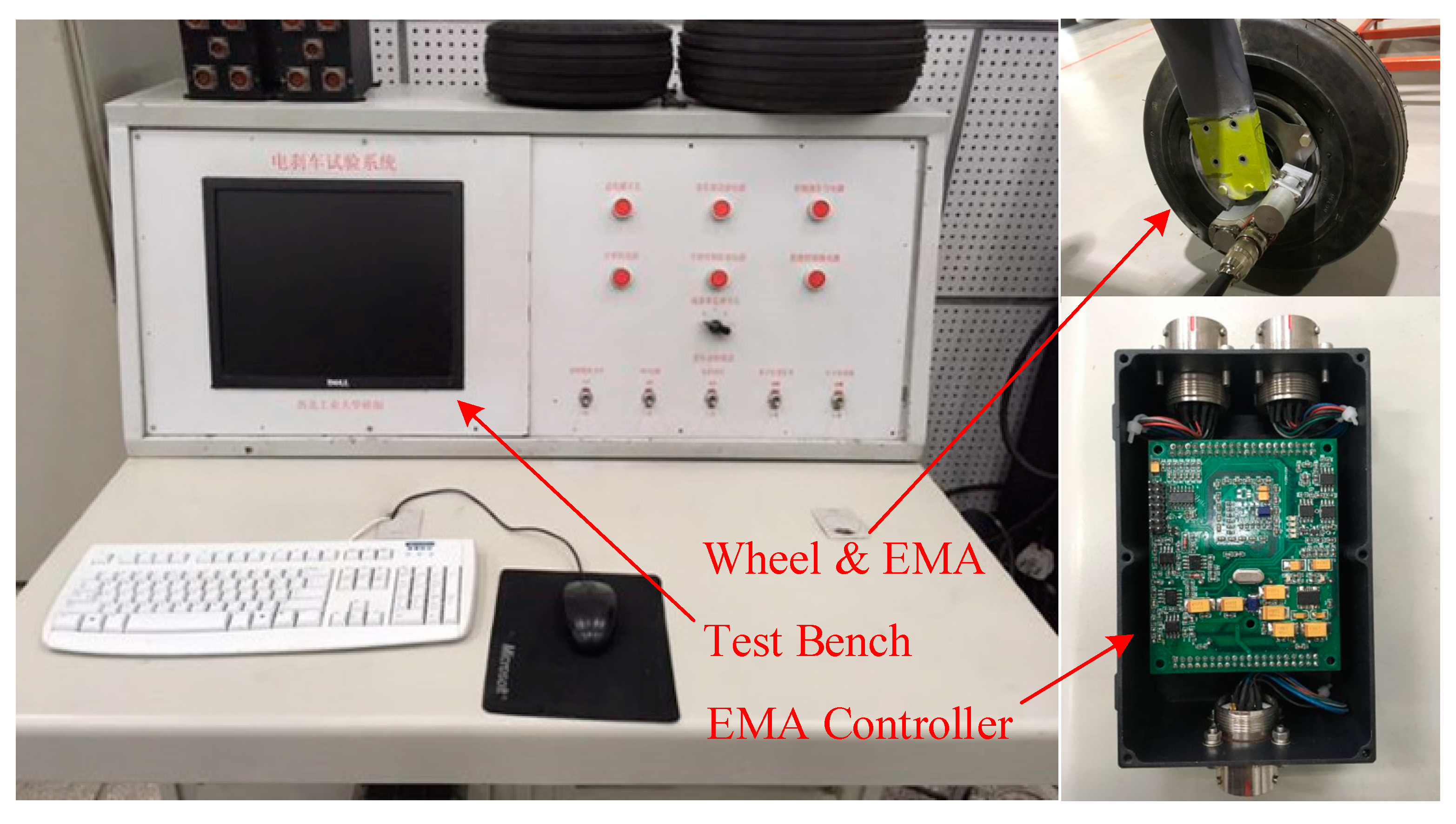
This section describes the validation of the designed ABS controller and EMA controller via experiments. As it is difficult to test the ABS controller in an actual UAV, a hardware in loop (HIL) test bench is built, which consists of two parts: the software and hardware [35]. The software part includes the UAV model and the upper computer, while the hardware part includes the ABS controller, EMA controller, EMA, and the wheel. The UAV model is built by using Simulink and downloaded to the simulation board to realize the simulation of the braking process, and then the velocity signal from the UAV model is transmitted to the ABS controller. After receiving the velocity signal, the ABS controller calculates the real-time slip ratio and outputs the reference braking pressure signal. Subsequently, the EMA controller receives the reference pressure signal and drives the EMA to realize the corresponding braking pressure. The HIL test bench of the electric braking system is shown in Figure 7. It should be noted that the generation of this paper is based on an actual engineering project, in which the unit of the braking pressure is kg, and so the unit of the braking pressure in this paper is the same.

The experiments consist of two parts: the braking pressure performance of the EMA controller, and the slip ratio control performance of the ABS controller under different runway conditions (dry, icy). The adhesive coefficient between the wheel and runway is calculated using the Burckhardt model:

$$\mu (\lambda )=c_1(1-e^{-c_2\lambda })-c_3\lambda$$

(37)

where $c_1$, $c_2$ and $c_3$ are constants, and they take different values for the various runway conditions.

The parameters for the UAV model and the EMA model are listed in

Table 2. Main parameters of the UAV model and EMA model.

Name	Description	Value	Name	Description	Value
$a$	Distance between front wheel and center of gravity of UAV	2.1 m	$b$	Distance between back wheel and center of gravity of UAV	1.6 m
$h$	Distance between ground and center of gravity of UAV	1.5 m	$I_w$	Moment of inertia of the back wheel	0.3 kg·m2
$g$	Gravity acceleration	9.8 m/s2	$n$	Number of the back wheels	2
$C_L$	Aerodynamic lift coefficient	0.66	${\rho }_a$	Air density	1.2 g/L
$S_L$	Aerodynamic lift area	5.1 m2	$C_P$	Aerodynamic drag coefficient	0.15
$m$	Weight of UAV	650 kg	$S_P$	Aerodynamic drag area	3.7 m2
$r$	The radius of the back wheel	0.18 m	$k_T$	Torque constant	0.3 N·m/A
$B_v$	Viscous damping coefficient	0.02 N·m/rad	$J$	Inertia moment of BLDCM	0.0002 Kg·m2
$c_b$	Stiffness coefficient of brake disc	5 × 106 N/m	$k_{emf}$	Back electromotive force constant	0.5 V·rad/s
$R$	Stator winding resistance	2.1 Ω	$\eta$	The transmission ratio of EMA	21
$L$	Stator winding inductance	1.2 mH	$L_0$	The lead of the ball screw	0.003 m

. The control parameters of the ABS controller and EMA controller are selected as follows: $k_1=60$, $\alpha =\beta =2$, $l=3$, $n_0/m_0=3/5$, $k_2^{*}=10$, ${\tau }_1^{*}=6$, ${\tau }_2=18$, and $n/m=5/7$.

4.1. Experimental Results for the EMA

First, the dynamic pressure performance of the EMA controller is tested, and two sets of controlled experiments are conducted. The signal from a signal generator is used as the reference pressure signal, and the experimental results are shown in Figure 8 and Figure 9.

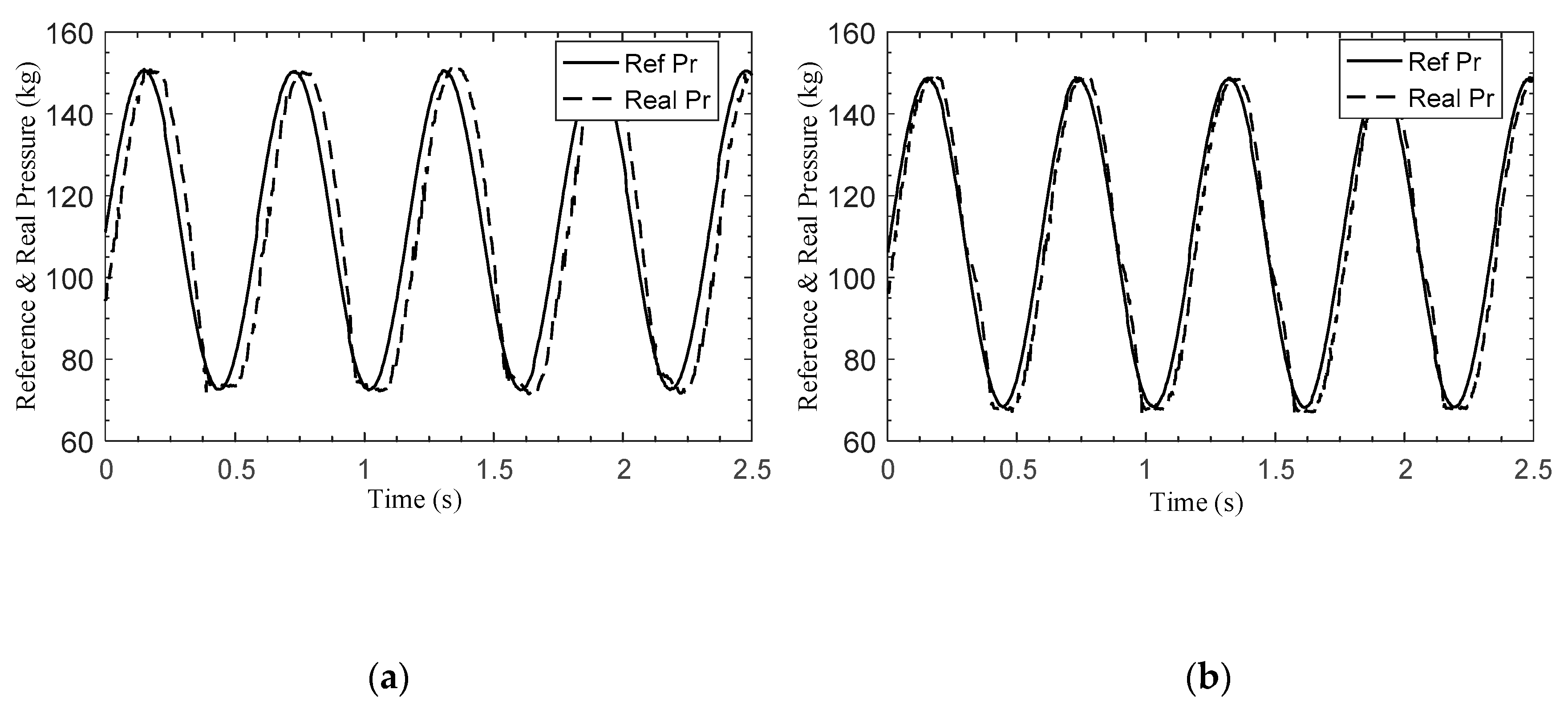
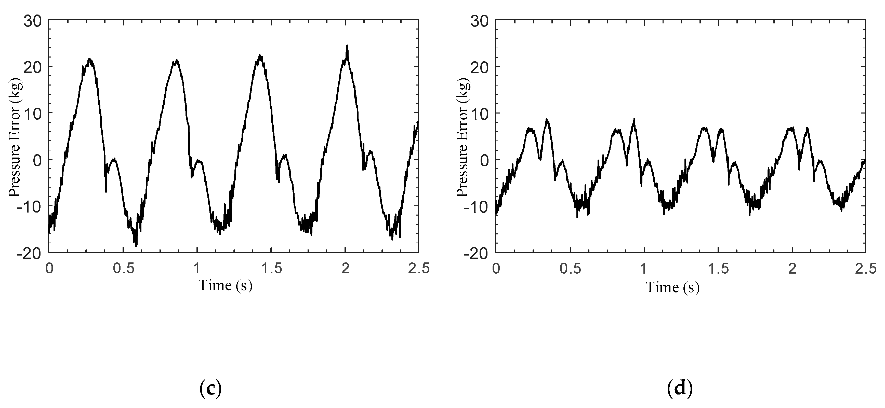
The first set of the controlled experiments is between the proposed control method and the traditional proportional integral derivative (PID) control method. A sine wave signal is used as the reference pressure signal. The transfer function of the PID controller is shown in (38).

$$C(s)=K_p+K_i/s+K_{d}s$$

(38)

Due to the particularity of the electric braking system, the parameters of the PID controller are designed in two stages, as follows: when the braking pressure is increasing, the parameters are $K_p=18$, $K_i=0.2$ and $K_d=0.5$; when the braking pressure is decreasing, the parameters are $K_p=12$, $K_i=0.13$ and $K_d=0.2$. The controlled experimental results are shown in Figure 8.

The frequency and amplitude range of the reference pressure signal are 2 Hz and 70–150 kg. The reference pressure and actual pressure of the two control methods are shown in Figure 8a,b, and the pressure errors are shown in Figure 8c,d. It can be seen from Figure 8a,b that the proposed control algorithm demonstrates a better tracking accuracy and smaller phase delays, which are the advantages of the fast convergence of the sliding mode characteristics. The pressure error comparison shown in Figure 8c,d indicates that the sliding mode controller makes the controller more responsive to large ranges of braking pressure, which leads to a smaller tracking error than that achieved with the traditional control method.

Then, the second set of controlled experiments is conducted with the proposed sliding mode control method, one with the fuzzy corrector and the other one without. A triangular wave signal is used as the reference signal. The frequency of the reference pressure signal was 2 Hz and the amplitude ranged from 20 kg to 100 kg. The experimental results are shown in Figure 9; it can be found that the major role of the fuzzy corrector is to reduce the chattering of the braking pressure, especially at the switching point when the direction of the braking pressure changes. The pressure errors in Figure 9c,d also demonstrate that the fuzzy corrector can reduce the tracking error and the system chattering significantly.

4.2. HIL Experimental Results for the Slip Ratio (Dry Runway Condition)

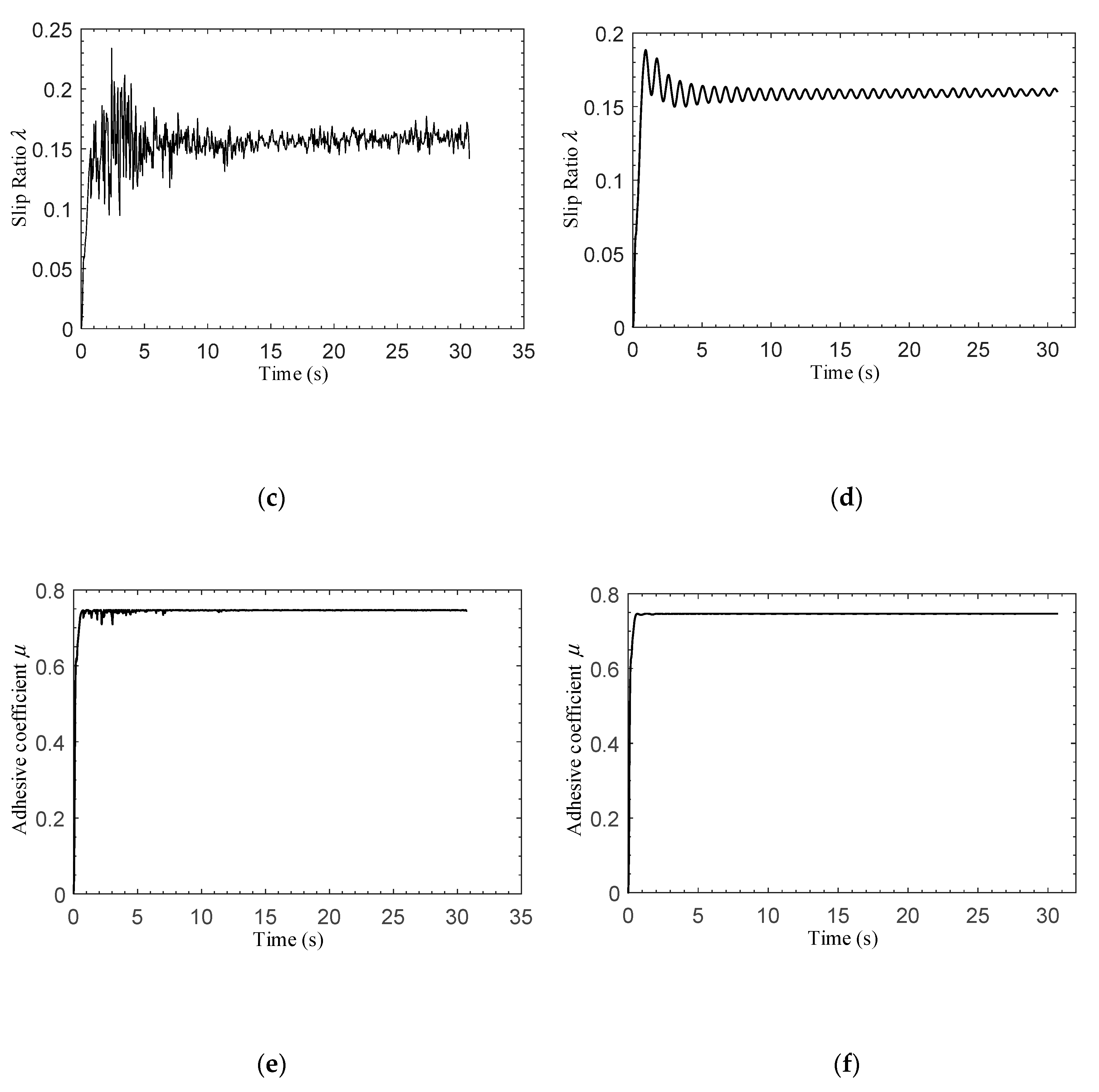
After the EMA experiments, the HIL experiments are conducted to verify the effectiveness of the ABS controller. The initial UAV speed and wheel speed are both 72 m/s, which implies that the initial value of the slip ratio is 0. The reference optimal value of the slip ratio under dry runway conditions is set to ${\lambda }^{*}=0.161$, when the adhesive coefficient, $\mu$, between the wheel and runway reaches the maximum value of 0.746, and the maximum upper value of the slip ratio is set to ${\lambda }_{\max }=0.2$. The slip ratio control performance of the traditional PID control method and the proposed control method under dry runway conditions are shown in Figure 10.

It can be seen from Figure 10a,b that the wheel velocity oscillates to a certain extent during the early stages of the braking process, and the proposed controller can effectively suppress the oscillation compared with the PID controller. The comparison between the slip ratios of the two control methods, as shown in Figure 10c,d, indicates that the proposed control method can ensure the control stability of the ABS controller, and the slip ratio is constrained to $\lambda <{\lambda }_{\max }$, so that the lateral stability of the UAV during the braking process can be guaranteed by using the proposed control strategy. The adhesive coefficient experimental results shown in Figure 10e,f also indicate that the proposed control method has a better control effect than that of the traditional method.

4.3. HIL Experimental Results for the Slip Ratio (Icy Runway Condition)

The icy runway is an extremely adverse environment for the landing of a UAV. Thus, a more advanced braking mechanism and ABS control strategy are necessary [36]. The reference optimal value of the slip ratio under icy runway conditions is set to ${\lambda }^{*}=0.054$, when the adhesive coefficient, $\mu$, between the wheel and runway reaches the maximum value of 0.2068, and the maximum upper value of the slip ratio is set to ${\lambda }_{\max }=0.07$. The corresponding experimental results are shown in Figure 11.

The adhesive coefficient between the wheel and runway under icy runway conditions is much smaller. As the traditional PID control method cannot restrict the slip ratio value due to the limitation of the algorithm itself, this leads to a bad control effect of the UAV braking system and the violent oscillation of the wheel velocity in Figure 11a. At the same time, the slip ratio and the adhesive coefficient between the wheel and runway also fluctuate in a large range, along with the wheel velocity, as shown in Figure 11c,e. When using the ABS controller proposed in this paper, as the BLF selected in the antiskid control law has good constraint effects of the slip ratio, the UAV braking system will still have good control stability under the icy runway conditions. The wheel velocity, slip ratio and adhesive coefficient between the wheel and runway can also be relatively stable, as shown in Figure 11b,d,f, which greatly enhances the lateral stability of the UAV when landing under icy runway conditions.

5. Conclusions

To achieve a high-performance braking pressure control for the UAV, a novel control strategy for the antiskid braking system is established. According to the design method of the backstepping control strategy, the antiskid braking system is divided into two subsystems: the ABS model and the EMA model. Then, the corresponding control objectives are proposed, and the control strategies are formulated based on the characteristics of the models. A BLF-based backstepping control strategy is proposed according to the constrained control requirements of the slip ratio, and a power fast terminal sliding mode control method is used to achieve high-performance braking pressure control. Furthermore, a fuzzy corrector is built to adjust the control parameters of the EMA controller in real-time. The following conclusions are obtained.

The proposed ABS controller can constrain the slip ratio within a stable range and outputs the braking pressure reference signal. Then, the power fast terminal sliding mode-based EMA controller can drive the ball screw to squeeze the brake disc and realize the braking action. The analysis shows that the proposed power fast terminal sliding mode control strategy has a power terminal characteristic, which allows a faster convergence on the equilibrium point with high precision. The slip ratio control strategy has the advantages of high stability and smooth control characteristics, and the BLF-based control strategy can constrain the slip ratio at its boundaries, which makes it different from the traditional control method.

The experimental results show that the proposed EMA controller can improve the servo performance and response speed of the EMA, and the fuzzy corrector reduces the system chattering caused by the sliding mode algorithm, especially at the switching point when the direction of the braking pressure changes. In the HIL experiments, the ABS controller exhibits a strong capability of constraining the actual slip ratio value, which can ensure the achievement of the maximum adhesive coefficient and braking stability under various runway conditions.

Furthermore, in the force analysis during the braking process of the UAV, the lateral motion of the UAV is neglected and only the longitudinal motion is considered. However, under practical working conditions, the lateral motion of the UAV is inevitable. In the following research, we will perfect the mathematical model of the UAV by combining the braking system with the front wheel steering system, so as to enhance the engineering application of the study.