3D Spatial Characteristics of C-V2X Communication Interference

Abstract

In C-V2X (cellular vehicle-to-everything) communication networks, dense spatial reuse of the available radio spectrum is required to achieve efficient spectral usage. Spectrum reuse causes severe network interference where signals from many undesired transmitters are aggregated at a receiver. This paper investigates the 3D spatial characteristics of C-V2X communication interference in the angular domain. A 3D GIDM (Gaussian interference distribution model) is proposed, and the corresponding interference APD (angular power density) is given. Then, the closed-form expressions of some key spatial statistics of interference are derived based on the interference APD. Finally, the closed-form expressions of the probability density function and spatial correlation function of SIR (signal–to–interference ratio) are derived based on the 3D multipath APD model and spatial statistics of the Rice channel. Simulation analysis shows that 3D spatial angular directions have significant effect on these spatial statistics of interference and the spatial correlation function of SIR. The results provide useful insight on the analysis and design of the interference-limited networks.

1. Introduction

C-V2X (cellular vehicle-to-everything) communication is essential for redefining transportation by providing real-time, highly reliable, and actionable information flows to enable safety, mobility, and environmental applications [1]. C-V2X communication networks comprise a huge number of spatially scattered nodes, and the high-density spectrum spatial multiplexing is the main method to improve spectrum utilization. However, C-V2X communication networks become interference-limited due to the frequency reuse. An appropriate interference model is of great significance to the design and performance enhancement of C-V2X communication systems, and it is also a research hotspot in the field of wireless communication. However, the complex and changeable signal propagation environment brings severe challenges to the study of the 3D model and spatial characteristics of C-V2X communication interference.

A lot of work has been done in various ways in the field of wireless communication interference modeling and analysis. The interference modeling and characteristic research results of cellular network, ad hoc network, and D2D (Device–to–Device) communication have important reference significance for the corresponding research of C-V2X communication. A circular interference model that aggregates given interferer topologies to power profiles along circles was proposed in [2] for heterogeneous cellular networks. A statistical model for quantifying the aggregate interference in heterogeneous cellular networks was proposed, and its impact on system performance was evaluated in [3]. Interference from static cellular cooperation using the nearest neighbor model was analyzed in [4]. Interference was modeled using hierarchical spatial clustering of terrain and user density maps in [5]. Interference prediction was investigated in [6] in a mobile ad hoc network with a finite number of nodes by proposing and using a general-order linear model for node mobility. HetNet interference was modeled and analyzed using Poisson cluster processes in [7]. Efficient simulation laws for the tail of the interference in a simple wireless ad hoc network model were provided in [8] considering node locations distributed according to a Poisson point process and various classes of light-tailed fading distributions. Average received interference power of D2D communication in the cellular network was analyzed in [9]. The interference graph construction for D2D communications in cellular networks was studied, and an interference graph construction protocol was proposed in [10]. Mathematical characteristics of the uplink interference region in D2D communications underlaying cellular networks were analyzed in [11]. A cross-layer model was established for D2D communications underlaying cellular network to characterize the realistic interference scenario in [12]. The impact of co-channel interference on the performance of V2V (vehicle–to–vehicle) communication was investigated based on 5.9 GHz real-world measurements conducted at intersections under LoS (line-of-sight) and NLoS (non-line-of-sight) conditions in [13]. The effect of hidden terminal interference on safety-critical traffic in vehicular ad hoc networks was investigated in [14]. A theoretical interference model of V2V communications at an intersection that uses a transmission power control method was proposed in [15]. The influence of interference in an inter-vehicular communication system was studied, and the interfering links were modeled using the multiple scattering radio channel in [16]. Interference signal approximations for system performance predictions and the impact on the IEEE 802.11p system in terms of bit and packet error probability and packet delays were analyzed in [17]. Methodology, experiment configuration, and final results from a set of measurements executed in order to validate the interference model assumptions adopted when simulating wireless networks with NS-3 were described in [18]. A novel network description method named the interference azimuth spectrum was proposed to determine the fundamental second-order small-scale fading statistics in the 2D angular domain in [19] and [20].

Since the heights of the vehicle nodes are different, and the signal is also scattered by the scatterers in the 3D space, the C-V2X communication interference is distributed in the 3D space. However, the model and characteristics of C-V2X communication interference have rarely been investigated so far in the 3D angular domain according to the above analysis. Therefore, this paper mainly investigates spatial characteristics of C-V2X communication interference in the 3D angular domain and obtains the effect of 3D spatial angular directions (i.e., azimuth angle and elevation angle) on spatial statistics of interference and SIR (signal–to–interference ratio). This paper strives to alleviate the current lack of analytical studies by proposing a 3D GIDM (Gaussian interference distribution model), giving the corresponding interference APD (angular power density) and deriving the closed-form expressions of some key spatial statistics of interference and SIR in the 3D angular domain.

The remainder of the paper is organized as follows. Section 2 proposes a 3D GIDM and gives the corresponding interference APD. Section 3 derives some key spatial statistics of interference. Section 4 derives the PDF (probability density function) and SCF (spatial correlation function) of the SIR. Discussions on obtained simulation results are provided in Section 5. Finally, conclusions are mentioned in Section 6.

2. 3D GIDM and Interference APD

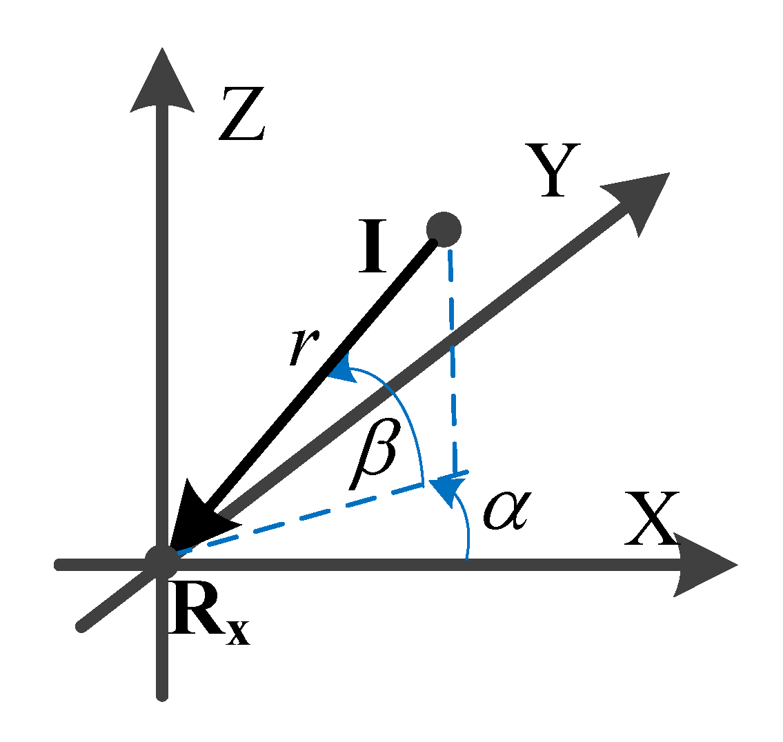
2.1. 3D GIDM

Figure 1 shows the 3D GIDM to describe the interference power distribution at the receiver ${\mathrm{R}}_{\mathrm{X}}$. The 3D GIDM is based on the following assumptions and settings:

(1)

the closer the interference signal to the receiving end, the stronger the influence, so the incoming interference power is assumed to obey the Gaussian distribution centered on the receiver in the 3D spatial distance [21];

(2)

since large-scale C-V2X communication networks have many nodes, it is assumed that the number of interference waves tends to infinity, and the multipath channel modeling theory can be used to study the spatial statistical characteristics of interference [19,20].

In Figure 1, I is the interferer if the interferer (base station or other terminal node) and ${\mathrm{R}}_{\mathrm{X}}$ have the LoS path, and I is the last scatterer before the arrival of the interference signal if the interferer and ${\mathrm{R}}_{\mathrm{X}}$ have no LoS path. $\alpha \in \left[0,2\mathsf{\pi }\right]$ and $\beta \in \left[0,\mathsf{\pi }/2\right]$ are the azimuth angle and elevation angle of the interference wave, respectively. $r$ is the distance from I to ${\mathrm{R}}_{\mathrm{X}}$. $\sigma$ is the standard deviation of the Gaussian distribution.

“Small probability events” generally refer to events with a probability of less than 5%, while Gaussian distribution variables with a mean of zero fall below $\left[-3\sigma ,3\sigma \right]$ with a probability of less than 0.3%. In practical problems, it is often assumed that the corresponding event does not occur. Basically, the interval $\left[-3\sigma ,3\sigma \right]$ can be regarded as the actual possible range of the Gaussian random variable. This is called the $3\sigma$ principle of the Gaussian distribution. Therefore, according to the $3\sigma$ principle of the Gaussian distribution, the maximum effective value of $r$ in Figure 1 is $3\sigma$.

2.2. Interference APD

Since the incoming interference power is assumed to obey the Gaussian distribution in 3D space, its expression is

$$f_G\left(x,y,z\right)=\frac{A_0}{\sqrt{2\pi }\sigma }\exp \left(-\frac{x^2+y^2+z^2}{2{\sigma }^2}\right)$$

(1)

where $f_G\left(x,y,z\right)$ is the spatial Gaussian distribution in Cartesian coordinates, and $z\ge 0$. $A_0$ is a constant used to ensure that $f_G\left(x,y,z\right)$ is integrated into 1 in the 3D space. In actual communication, the distributions of interferers (or interference scatterers) in the horizontal and vertical directions are different. Generally, the smaller the elevation angle, the more interferers (or interference scatterers) exist, and the greater the impact the interference causes. Therefore, the standard deviation of the Gaussian distribution needs to be controlled separately in the horizontal and vertical directions. This paper assumes that the standard deviation of the Gaussian distribution in the horizontal direction is ${\sigma }_{\alpha }$, the standard deviation in the vertical direction is ${\sigma }_{\beta }$, and ${\sigma }_{\alpha }>{\sigma }_{\beta }$. Then the maximum effective value of $r$ in the vertical direction is $3{\sigma }_{\beta }$, and the maximum effective value of $r$ in the horizontal direction is $3{\sigma }_{\alpha }$. The 3D standard deviation $\sigma$ can be expressed as

$$\sigma =\sqrt{\frac{{\sigma }_{\alpha }^2{\sigma }_{\beta }^2}{{\sigma }_{\beta }^2{\cos }^2\beta +{\sigma }_{\alpha }^2{\sin }^2\beta }}$$

(2)

Equation (1) in Cartesian coordinates can be converted to an equation in spherical coordinates by the Jacobian formula [22]:

$$P_G\left(r,\alpha ,\beta \right)={\frac{f_G\left(x,y,z\right)}{\left|J\left(x,y,z\right)\right|}|}_{\begin{array}{l}x=r\cos \beta \cos \alpha \\ y=r\cos \beta \sin \alpha \\ z=r\sin \beta \end{array}}=f_G\left(x,y,z\right)r^2\cos \beta =\frac{A_0{r}^2}{\sqrt{2\pi }\sigma }\exp \left(-\frac{r^2}{2{\sigma }^2}\right)\cos \beta$$

(3)

Then the interference APD can be calculated as

$$P_G\left(\alpha ,\beta \right)={\displaystyle {\int }_0^{\infty }{p}_G\left(r,\alpha ,\beta \right)dr}=\frac{A_0\cos \beta }{\sqrt{2\pi }\sigma }{\displaystyle {\int }_0^{\infty }{r}^2\exp \left(-\frac{r^2}{2{\sigma }^2}\right)dr}$$

(4)

because

$${\displaystyle \int x^2}\exp \left(-a{x}^2\right)dx=-\frac{x}{2a}\exp \left(-a{x}^2\right)+\frac{\sqrt{a\pi }}{4a^2}\mathrm{erf}\left(\sqrt{a}x\right)$$

(5)

where $\mathrm{erf}(·)$ is the error function, $\mathrm{erf}\left(x\right)=\frac{2}{\sqrt{\pi }}{\displaystyle {\int }_0^x\exp \left(-t^2\right)}dt$. Let $x=r$ and $a=1/2{\sigma }^2$, using the conclusion of Equation (5), and the closed expression of interference APD can be written as

$$P_G\left(\alpha ,\beta \right)=\frac{A_0\cos \beta }{\sqrt{2\pi }\sigma }{\left[-{\sigma }^{2}r\exp \left(-\frac{r^2}{2{\sigma }^2}\right)+\frac{\sqrt{2\pi }{\sigma }^3}{2}\mathrm{erf}\left(\frac{\sqrt{2}}{2\sigma }r\right)\right]||}_0^{\infty }=\frac{A_0{\sigma }^2\cos \beta }{2}=\frac{A_0{\sigma }_{\alpha }^2{\sigma }_{\beta }^2\cos \beta }{2{\sigma }_{\beta }^2{\cos }^2\beta +2{\sigma }_{\alpha }^2{\sin }^2\beta }$$

(6)

Therefore, the interference APD in the vertical direction is

$$P_G\left(\beta \right)={\displaystyle {\int }_0^{2\pi }\frac{A_0{\sigma }_{\alpha }^2{\sigma }_{\beta }^2\cos \beta }{2{\sigma }_{\beta }^2{\cos }^2\beta +2{\sigma }_{\alpha }^2{\sin }^2\beta }d\alpha }=\frac{A_0\pi {\sigma }_{\alpha }^2{\sigma }_{\beta }^2\cos \beta }{{\sigma }_{\beta }^2{\cos }^2\beta +{\sigma }_{\alpha }^2{\sin }^2\beta }$$

(7)

The interference APD in the horizontal direction is

$$P_G\left(\alpha \right)={\displaystyle {\int }_0^{\frac{\pi }{2}}\frac{A_0{\sigma }_{\alpha }^2{\sigma }_{\beta }^2\cos \beta }{2{\sigma }_{\beta }^2{\cos }^2\beta +2{\sigma }_{\alpha }^2{\sin }^2\beta }d\beta }=\frac{1}{2\pi }{\displaystyle {\int }_0^{\frac{\pi }{2}}{P}_G\left(\beta \right)d\beta }=\frac{1}{2\pi }$$

(8)

because the integral of the interference APD is 1, therefore

$$\begin{array}{ll}{\displaystyle {\int }_0^{\frac{\pi }{2}}{P}_G\left(\beta \right)d\beta }& ={\displaystyle {\int }_0^{\frac{\pi }{2}}\frac{A_0\pi {\sigma }_{\alpha }^2{\sigma }_{\beta }^2\cos \beta }{{\sigma }_{\beta }^2{\cos }^2\beta +{\sigma }_{\alpha }^2{\sin }^2\beta }d\beta }\\ & =\frac{A_0\pi {\sigma }_{\alpha }^2{\sigma }_{\beta }\left[\left({\sigma }_{\alpha }-A_3\right)A_2\arctan \left({\sigma }_{\beta }/A_1\right)-\left({\sigma }_{\alpha }+A_3\right)A_1\arctan \left({\sigma }_{\beta }/A_2\right)\right]}{A_1{A}_2{A}_3}=1\end{array}$$

(9)

where $A_1=\sqrt{-{\sigma }_{\beta }^2+2{\sigma }_{\alpha }\left({\sigma }_{\alpha }-\sqrt{{\sigma }_{\alpha }^2-{\sigma }_{\beta }^2}\right)}$, $A_2=\sqrt{-{\sigma }_{\beta }^2+2{\sigma }_{\alpha }\left({\sigma }_{\alpha }+\sqrt{{\sigma }_{\alpha }^2-{\sigma }_{\beta }^2}\right)}$, $A_3=\sqrt{{\sigma }_{\alpha }^2-{\sigma }_{\beta }^2}$. So, the expression of $A_0$ is $\frac{A_1{A}_2{A}_3/\pi {\sigma }_{\alpha }^2{\sigma }_{\beta }}{\left({\sigma }_{\alpha }-A_3\right)A_2\arctan \left({\sigma }_{\beta }/A_1\right)-\left({\sigma }_{\alpha }+A_3\right)A_1\arctan \left({\sigma }_{\beta }/A_2\right)}$.

3. Spatial Statistics of Interference

3.1. 3D Shape Factors

According to the definition in [23], the l-th degree and m-th order unnormalized complex spherical harmonic coefficient $S_l^m$ for the interference APD $P_G\left(\alpha ,\beta \right)$ can be derived as

$$\{\begin{array}{l}{S}_0^0=\frac{A_0{\pi }^2{\sigma }_{\alpha }^2{\sigma }_{\beta }}{2\left({\sigma }_{\beta }+{\sigma }_{\alpha }\right)}, S_1^0=\frac{A_0\pi {\sigma }_{\alpha }^2{\sigma }_{\beta }^2}{{\left({\sigma }_{\beta }^2-{\sigma }_{\alpha }^2\right)}^{3/2}}\left\{\sqrt{{\sigma }_{\beta }^2-{\sigma }_{\alpha }^2}+{\sigma }_{\alpha }\arctan \left[\frac{2{\sigma }_{\alpha }^2-{\sigma }_{\beta }^2}{2{\sigma }_{\alpha }\sqrt{{\sigma }_{\beta }^2-{\sigma }_{\alpha }^2}}\right]-{\sigma }_{\alpha }\arctan \left[\frac{{\sigma }_{\alpha }}{\sqrt{{\sigma }_{\beta }^2-{\sigma }_{\alpha }^2}}\right]\right\}\hfill \\ S_1^1=0, S_2^0=\frac{A_0{\pi }^2{\sigma }_{\alpha }^2{\sigma }_{\beta }\left({\sigma }_{\beta }-2{\sigma }_{\alpha }\right)}{12{\left({\sigma }_{\beta }+{\sigma }_{\alpha }\right)}^2}, S_2^1=0, S_2^2=0\hfill \end{array}$$

(10)

Therefore, the 3D shape factors defined in [24] can be derived as

$$\Lambda =\sqrt{1-\frac{{\left(S_1^0\right)}^2+{\left|S_1^1\right|}^2}{{\left(S_0^0\right)}^2}}=\sqrt{1-\frac{{\left(S_1^0\right)}^2}{{\left(S_0^0\right)}^2}}$$

(11)

$$\xi =\frac{\frac{3}{2}{S}_2^0{S}_0^0-{\left(S_1^0\right)}^2+\frac{1}{2}{\left|S_1^1\right|}^2}{{\left(S_0^0\right)}^2-{\left(S_1^0\right)}^2-{\left|S_1^1\right|}^2}=\frac{3S_2^0{S}_0^0/2-{\left(S_1^0\right)}^2}{{\left(S_0^0\right)}^2-{\left(S_1^0\right)}^2}$$

(12)

$$\chi =\frac{2\left|S_2^1{S}_0^0-S_1^0{S}_1^1\right|}{{\left(S_0^0\right)}^2-{\left(S_1^0\right)}^2-{\left|S_1^1\right|}^2}=0$$

(13)

$$\gamma =\frac{\left|S_2^2{S}_0^0-{\left(S_1^1\right)}^2\right|}{{\left(S_0^0\right)}^2-{\left(S_1^0\right)}^2-{\left|S_1^1\right|}^2}=0$$

(14)

$${\alpha }_{\beta 45}^{\max }=\arg \left\{S_2^1{S}_0^0-S_1^0{S}_1^1\right\}=\arg \left\{0\right\}$$

(15)

$${\alpha }_{\beta 0}^{\max }=\frac{1}{2}\arg \left\{S_2^2{S}_0^0-{\left(S_1^1\right)}^2\right\}=\frac{1}{2}\arg \left\{0\right\}$$

(16)

where $\Lambda$, $\xi$, $\chi$, $\gamma$, ${\alpha }_{\beta 45}^{\max }$ and ${\alpha }_{\beta 0}^{\max }$ are the 3D angular spread, elevational constriction, 45° inclined constriction, azimuthal constriction, azimuth of maximum fading at 45° elevation, and azimuth of maximum fading at zero elevation, respectively. $\Lambda \in \left[0,1\right]$ is a measure of how interference power concentrates about a single direction; $\xi \in \left[-0.5,1\right]$ shows how much the interference APD is concentrated on a single elevational cone or along two paths at the same azimuth and opposite elevations; $\chi =0$ shows the interference APD is horizontal or vertical mirror symmetrical; $\gamma =0$ shows two-path interference APD has no significant difference in the azimuth direction; Equations (15) and (16) indicate that ${\alpha }_{\beta 45}^{\max }$ and ${\alpha }_{\beta 0}^{\max }$ do not exist.

3.2. Interference Fading Rate Variance

Since the mean derivative of a stationary process is zero, the variance of the fading rate of a received complex voltage is the simplest statistic that measures the fading rate, and it can be derived as [24].

$$\begin{array}{ll}{\sigma }_I^2\left(\alpha ,\beta \right)& =\frac{4{\pi }^2{\Lambda }^2{P}_I}{3{\lambda }^2}\left\{1+\frac{3}{2}\left[\xi \left(2{\sin }^2\beta -\frac{2}{3}\right)+\chi \sin 2\beta \cos \left(\alpha -{\alpha }_{\beta 45}^{\max }\right)+\gamma {\cos }^2\beta \cos 2\left(\alpha -{\alpha }_{\beta 0}^{\max }\right)\right]\right\}\\ & =\frac{4{\pi }^2{\Lambda }^2{P}_I\left[1+\xi \left(3{\sin }^2\beta -1\right)\right]}{3{\lambda }^2}\end{array}$$

(17)

where $P_I$ is the total received interference power in a local volume, and $\lambda$ is the carrier wavelength. According to Equation (17), the maximum and minimum values of ${\sigma }_I^2\left(\alpha ,\beta \right)$ are respectively,

$${\sigma }_{I,\max }^2=\max \left\{\frac{4{\pi }^2{\Lambda }^2{P}_I\left[1+\xi \left(3{\sin }^2\beta -1\right)\right]}{3{\lambda }^2}\right\}=\frac{4{\pi }^2{\Lambda }^2{P}_I\left(1+2\xi \right)}{3{\lambda }^2},\beta =\frac{\pi }{2}$$

(18)

$${\sigma }_{I,\min }^2=\min \left\{\frac{4{\pi }^2{\Lambda }^2{P}_I\left[1+\xi \left(3{\sin }^2\beta -1\right)\right]}{3{\lambda }^2}\right\}=\frac{4{\pi }^2{\Lambda }^2{P}_I\left(1-\xi \right)}{3{\lambda }^2},\beta =0$$

(19)

For the mobile receiver of C-V2X communication networks, it is often convenient to measure the variance of the fading rate in terms of the change over time. According to [25], the mean-squared time rate-of-change ${\sigma }_V^2\left(\alpha ,\beta \right)$ of a received complex voltage is equal to ${\sigma }_I^2\left(\alpha ,\beta \right)$ times the square of the moving speed $v_R$ of the receiver. Since this paper mainly studies the variation of interference and SIR, regardless of the specific amplitude, the moving speed $v_R$ of the receiver is set to 1, and ${\sigma }_I^2\left(\alpha ,\beta \right)$ is used instead of ${\sigma }_V^2\left(\alpha ,\beta \right)$ in the derivation of expressions below.

3.3. Interference Level Crossing Rate and Average Fade Duration

Each interference fading signal is assumed to obey Rayleigh distribution or Rice distribution. According to [26,27], the sum of multiple Rayleigh or Rice distributions can approximate a Nakagami-m distribution. Therefore, the total interference signal at the receiver ${\mathrm{R}}_{\mathrm{X}}$ obeys the Nakagami-m distribution. Ref. [20] has already derived the expressions of 2D spatial LCR (level crossing rate) and AFD (average fade duration) for a Nakagami-m fading signal, and the fading rate variance is only closely related to the space dimension. Therefore, the 3D LCR is

$$N_I\left({\rho }_N,\alpha ,\beta \right)=\frac{{\sigma }_I\left(\alpha ,\beta \right)}{\sqrt{\pi P_I}}\frac{m^{m-1/2}}{\Gamma \left(m\right)}{\rho }_N^{2m-1}\exp \left(-m{\rho }_N^2\right)=\frac{2\Lambda {\rho }_N^{2m-1}\sqrt{3\pi \left[1+\xi \left(3{\sin }^2\beta -1\right)\right]}}{3\lambda }\exp \left(-m{\rho }_N^2\right)$$

(20)

where ${\rho }_N=R_l/\sqrt{P_T}$ is the normalized threshold level, $R_l$ is the envelope threshold, $m$ is the Nakagami-m shape factor, and $\Gamma (·)$ is the Gamma function. By definition, the 3D AFD can be derived as

$$\begin{array}{ll}{\overline{l}}_I\left({\rho }_N,\alpha ,\beta \right)& =\frac{1}{N_I\left({\rho }_N,\alpha ,\beta \right)}{\displaystyle {\int }_0^R{P}_m\left(r\right)}dr=\frac{1}{N_I\left({\rho }_N,\alpha ,\beta \right)}\frac{\Gamma \left(m,m{\rho }_N^2\right)}{\Gamma \left(m\right)}\\ & =\frac{\sqrt{3\pi }\Gamma \left(m,m{\rho }_N^2\right)\lambda }{2\pi \Lambda {\rho }_N^{2m-1}\Gamma \left(m\right)\sqrt{1+\xi \left(3{\sin }^2\beta -1\right)}\exp \left(-m{\rho }_N^2\right)}\end{array}$$

(21)

where $P_m\left(r\right)$ is the PDF of the Nakagami-m distribution, and $\Gamma \left(·,·\right)$ is the incomplete Gamma function.

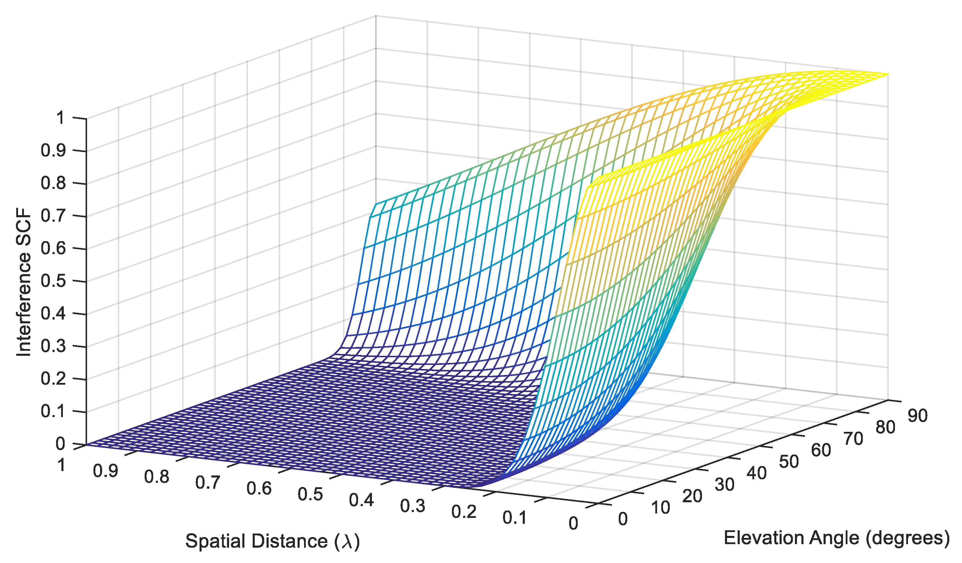
3.4. Interference Spatial Correlation and Coherence Distance

The interference envelope SCF can be defined as

$$R_I\left(r_c,\alpha ,\beta \right)=\frac{{\rm E}\left[r\left(p_0\right)r\left(p_0+r_c\overrightarrow{p}\right)\right]-{\left[{\rm E}\left(r\right)\right]}^2}{{\rm E}\left(r^2\right)-{\left[{\rm E}\left(r\right)\right]}^2}$$

(22)

where $E(•)$ is the statistical expectation operator, $p_0$ is any initial position, $\overrightarrow{p}$ is the unit direction vector, and $r_c$ is the spatial distance. Equation (22) can be approximated by a Mclaurin expansion [28]:

$$R_I\left(r_c,\alpha ,\beta \right)=1+\frac{{\displaystyle \sum _{n=1}^{\infty }\frac{{\left(-1\right)}^n{r}_c{}^{2n}}{\left(2n\right)!}}{\rm E}\left[{\left(\frac{d^{n}r}{d{r}_c{}^n}\right)}^2\right]}{{\rm E}\left(r^2\right)-{\left[{\rm E}\left(r\right)\right]}^2}=1-\frac{{\rm E}\left[{\left(\frac{dr}{d{r}_c}\right)}^2\right]}{2\left\{{\rm E}\left(r^2\right)-{\left[{\rm E}\left(r\right)\right]}^2\right\}}{r}_c{}^2+\cdots =1-\frac{{\sigma }_I^2\left(\alpha ,\beta \right)}{2V_m\left(r\right)}{r}_c{}^2+\cdots$$

(23)

where $V_m\left(r\right)$ is the variance of Nakagami-m distribution.

At the same time, SCF can also be approximated as an exponential function and its Mclaurin expansion is as follows:

$$R_I\left(r_c,\alpha ,\beta \right)\approx \exp \left[-a{\left(\frac{r_c}{\lambda }\right)}^2\right]\approx 1-a{\left(\frac{r_c}{\lambda }\right)}^2+\cdots$$

(24)

Let Equation (23) = Equation (24), and interference SCF can be obtained

$$R_I\left(r_c,\alpha ,\beta \right)\approx \exp \left[-\frac{{\sigma }_I^2\left(\alpha ,\beta \right)}{2V_m\left(r\right)}{r}_c{}^2\right]=\exp \left\{-\frac{2{\pi }^2{\Lambda }^{2}m{\Gamma }^2\left(m\right)\left[1+\xi \left(3{\sin }^2\beta -1\right)\right]}{3{\lambda }^2\left[m{\Gamma }^2\left(m\right)-{\Gamma }^2\left(m+\frac{1}{2}\right)\right]}{r}_c{}^2\right\}$$

(25)

If the SCF equals $\exp \left(-1\right)$ for the spatial distance $r_c$, the distance is defined as the coherence distance $D_I$,

$$D_I=\frac{\lambda \sqrt{6m}}{2m\pi \Lambda \Gamma \left(m\right)}\sqrt{\frac{m{\Gamma }^2\left(m\right)-{\Gamma }^2\left(m+\frac{1}{2}\right)}{1+\xi \left(3{\sin }^2\beta -1\right)}}$$

(26)

4. Spatial Statistics of SIR

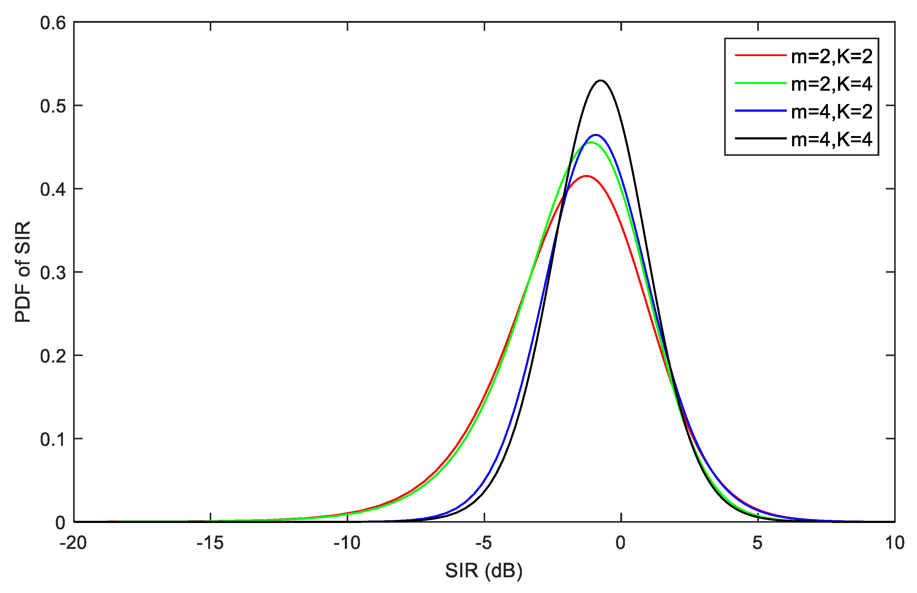
4.1. Probability Density Function of SIR

The useful signal $r_S$ at the receiver ${\mathrm{R}}_{\mathrm{X}}$ is assumed to obey the Rice distribution, and its average power is expressed as $P_S$. The total interference signal $r_I$ at ${\mathrm{R}}_{\mathrm{X}}$ obeys the Nakagami-m distribution, and its average power is expressed as $P_I$. Therefore, the SIR can be written as $\eta =r_S{}^2/r_I{}^2$.

According to [26,29], the square of the Nakagami-m distribution variable $r_I{}^2$ (i.e., the instantaneous power of $r_I$) obeys the Gamma distribution $\mathrm{G}\left(a_1,b_1\right)$,

$$f\left(x;a_1,b_1\right)=\frac{b_1{\left(b_{1}x\right)}^{b_1-1}\exp \left(-b_{1}x\right)}{\Gamma \left(a_1\right)}$$

(27)

where $a_1=m$, $b_1=m/P_I$. The mean of the Gamma distribution is $a_1/b_1$ and the variance is $a_1/b_1{}^2$.

The Rice distribution can be approximated as the Nakagami-m distribution when $K=\sqrt{m_s{}^2-m_s}/\left(m_s-\sqrt{m_s{}^2-m_s}\right)$ [26], and $K$ is the Rice K-factor defined as the ratio of the power contributions by the LoS path to the remaining multipath, $m_s$ is the Nakagami-m shape factor for Rice distribution. Therefore, the square of the Rice distribution variable also approximately obeys the Gamma distribution $\mathrm{G}\left(a_2,b_2\right)$, and $a_2=m_s={\left(K+1\right)}^2/\left(2K+1\right)$, $b_2=m_s/P_S={\left(K+1\right)}^2/\left[P_S\left(2K+1\right)\right]$. The mean and the variance of $\mathrm{G}\left(a_2,b_2\right)$ are $a_2/b_2$ and $a_2/b_2{}^2$, respectively.

The ratio of the two Gamma distribution variables $\mathrm{G}\left(a_1,b_1\right)/\mathrm{G}\left(a_2,b_2\right)$ obeys the compound Gamma distribution ${\beta }^{\prime }\left(a_1,a_2,1,b_2/b_1\right)$ which is a special case of the general beta basic distribution [30], and its expression is

$$f\left(x;a_3,b_3,1,c_3\right)={\beta }^{\prime }\left(a_3,b_3,1,c_3\right)=\frac{c_3{}^{b_3}{x}^{a_3-1}}{{\rm B}\left(a_3,b_3\right){\left(c_3+x\right)}^{a_3+b_3}}$$

(28)

where ${\rm B}\left(x,y\right)={\displaystyle {\int }_0^1{t}^{x-1}}{\left(1-t\right)}^{y-1}dt$ is beta function. Therefore, the PDF of SIR $\eta$ can be derived as

$$P\left(\eta \right)=\frac{{\left(b_2/b_1\right)}^{a_2}{\eta }^{a_1-1}}{{\rm B}\left(a_1,a_2\right){\left(b_2/b_1+\eta \right)}^{a_1+a_2}}=\frac{b_1{}^{a_1}{b}_2{}^{a_2}{\eta }^{a_1-1}}{{\rm B}\left(a_1,a_2\right){\left(b_2+b_1\eta \right)}^{a_1+a_2}},\{\begin{array}{l}{a}_1=m\hfill \\ b_1=m/P_I\hfill \\ a_2={\left(K+1\right)}^2/\left(2K+1\right)\hfill \\ b_2={\left(K+1\right)}^2/\left[P_S\left(2K+1\right)\right]\hfill \end{array}$$

(29)

The k-th order moment, mean and variance of SIR $\eta$ are respectively [30]

$${\rm E}\left[{\eta }^k\right]=\frac{b_2{}^k{\rm B}\left(a_2-k,a_1+k\right)}{b_1{}^k{\rm B}\left(a_1,a_2\right)},a_2>k$$

(30)

$${\rm E}\left[\eta \right]=\frac{a_1{b}_2}{b_1\left(a_2-1\right)},a_2>1$$

(31)

$$Var\left[\eta \right]=\frac{a_1{b}_2{}^2\left(a_1+a_2-1\right)}{b_1{}^2{\left(a_2-1\right)}^2\left(a_2-2\right)},a_2>2$$

(32)

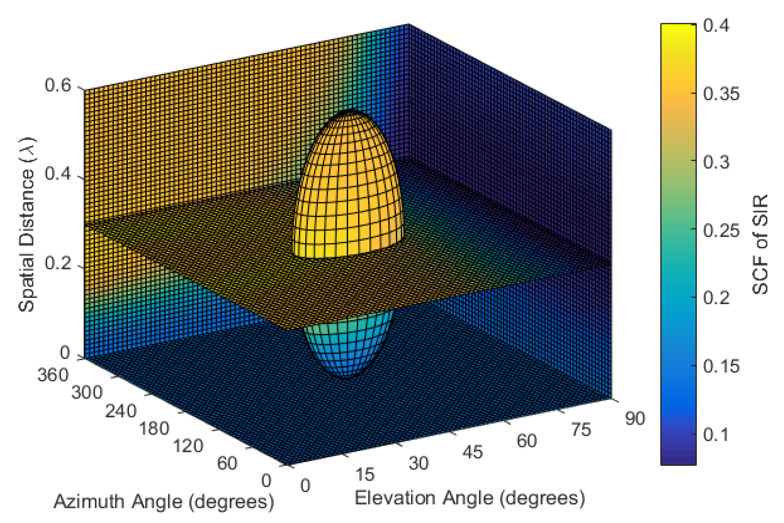
4.2. Spatial Correlation Function of SIR

Similar to the interference, the SCF of SIR can be defined as

$$R\left({\eta }_c,\alpha ,\beta \right)=\frac{{\rm E}\left[\eta \left(p_0\right)\eta \left(p_0+{\eta }_c\overrightarrow{p}\right)\right]-{\left[{\rm E}\left(\eta \right)\right]}^2}{{\rm E}\left({\eta }^2\right)-{\left[{\rm E}\left(\eta \right)\right]}^2}$$

(33)

where ${\eta }_c$ is the spatial distance.

According to Equations (30)–(32),

$${\rm E}\left({\eta }^2\right)-{\left[{\rm E}\left(\eta \right)\right]}^2=Var\left[\eta \right]=\frac{a_1{b}_2{}^2\left(a_1+a_2-1\right)}{b_1{}^2{\left(a_2-1\right)}^2\left(a_2-2\right)},a_2>2$$

(34)

$${\left[{\rm E}\left(\eta \right)\right]}^2=\frac{a_1{}^2{b}_2{}^2}{b_1{}^2{\left(a_2-1\right)}^2},a_2>1$$

(35)

For the convenience of derivation, let ${\Phi }_{\eta }\left({\eta }_c\right)=\eta \left(p_0\right)\eta \left(p_0+{\eta }_c\overrightarrow{p}\right)$, ${\Phi }_S\left({\eta }_c\right)=r_S\left(p_0\right)r_S\left(p_0+{\eta }_c\overrightarrow{p}\right)$ and ${\Phi }_I\left({\eta }_c\right)=r_I\left(p_0\right)r_I\left(p_0+{\eta }_c\overrightarrow{p}\right)$, then

$${\rm E}\left[{\Phi }_{\eta }\left({\eta }_c\right)\right]={\rm E}\left[\eta \left(p_0\right)\eta \left(p_0+{\eta }_c\overrightarrow{p}\right)\right]={\rm E}\left[\frac{r_S{}^2\left(p_0\right)}{r_I{}^2\left(p_0\right)}\frac{r_S{}^2\left(p_0+{\eta }_c\overrightarrow{p}\right)}{r_I{}^2\left(p_0+{\eta }_c\overrightarrow{p}\right)}\right]={\rm E}\left[\frac{{\Phi }_S{}^2\left({\eta }_c\right)}{{\Phi }_I{}^2\left({\eta }_c\right)}\right]$$

(36)

According to [28], Equation (36) can be approximated as

$$\begin{array}{ll}{\rm E}\left[{\Phi }_{\eta }\left({\eta }_c\right)\right]& ={\rm E}\left[\frac{{\Phi }_S{}^2\left({\eta }_c\right)}{{\Phi }_I{}^2\left({\eta }_c\right)}\right]\approx \frac{{{\rm E}}^2\left[{\Phi }_S\left({\eta }_c\right)\right]}{{{\rm E}}^2\left[{\Phi }_I\left({\eta }_c\right)\right]}+\frac{1}{2}\left[\frac{{\partial }^2{\Phi }_{\eta }\left({\eta }_c\right)}{\partial {\Phi }_S{}^2\left({\eta }_c\right)}{\sigma }_{{\Phi }_S\left({\eta }_c\right)}^2+\frac{{\partial }^2{\Phi }_{\eta }\left({\eta }_c\right)}{\partial {\Phi }_I{}^2\left({\eta }_c\right)}{\sigma }_{{\Phi }_I\left({\eta }_c\right)}^2\right]\\ & =\frac{{{\rm E}}^2\left[{\Phi }_S\left({\eta }_c\right)\right]}{{{\rm E}}^2\left[{\Phi }_I\left({\eta }_c\right)\right]}+\frac{1}{2}\left\{\frac{2}{{{\rm E}}^2\left[{\Phi }_I\left({\eta }_c\right)\right]}{\sigma }_{{\Phi }_S\left({\eta }_c\right)}^2+\frac{6{{\rm E}}^2\left[{\Phi }_S\left({\eta }_c\right)\right]}{{{\rm E}}^4\left[{\Phi }_I\left({\eta }_c\right)\right]}{\sigma }_{{\Phi }_I\left({\eta }_c\right)}^2\right\}\\ & \approx \frac{{{\rm E}}^2\left[{\Phi }_S\left({\eta }_c\right)\right]}{{{\rm E}}^2\left[{\Phi }_I\left({\eta }_c\right)\right]}+\frac{1}{{{\rm E}}^2\left[{\Phi }_I\left({\eta }_c\right)\right]}{\sigma }_{{\Phi }_S\left(0\right)}^2+\frac{3{{\rm E}}^2\left[{\Phi }_S\left({\eta }_c\right)\right]}{{{\rm E}}^4\left[{\Phi }_I\left({\eta }_c\right)\right]}{\sigma }_{{\Phi }_I\left(0\right)}^2\end{array}$$

(37)

where ${\sigma }_{{\Phi }_S\left({\eta }_c\right)}^2$ and ${\sigma }_{{\Phi }_I\left({\eta }_c\right)}^2$ are variances of ${\Phi }_S\left({\eta }_c\right)$ and ${\Phi }_I\left({\eta }_c\right)$, respectively. ${\Phi }_S\left(0\right)$ and ${\Phi }_I\left(0\right)$ obey the Gamma distribution, so

$${\sigma }_{{\Phi }_S\left(0\right)}^2={\rm E}\left[{\Phi }_S{}^2\left(0\right)\right]-{{\rm E}}^2\left[{\Phi }_S\left(0\right)\right]=\frac{a_2}{b_2{}^2}$$

(38)

$${\sigma }_{{\Phi }_I\left(0\right)}^2={\rm E}\left[{\Phi }_I{}^2\left(0\right)\right]-{{\rm E}}^2\left[{\Phi }_I\left(0\right)\right]=\frac{a_1}{b_1{}^2}$$

(39)

According to Equation (22),

$$\begin{array}{ll}{\rm E}\left[{\Phi }_I\left({\eta }_c\right)\right]& ={\rm E}\left[r_I\left(p_0\right)r_I\left(p_0+{\eta }_c\overrightarrow{p}\right)\right]\\ & =R_I\left({\eta }_c,\alpha ,\beta \right)\left\{{\rm E}\left(r_I{}^2\right)-{\left[{\rm E}\left(r_I\right)\right]}^2\right\}+{\left[{\rm E}\left(r_I\right)\right]}^2=R_I\left({\eta }_c,\alpha ,\beta \right)V_m+E_m{}^2\end{array}$$

(40)

where $V_m$ and $E_m$ are the variance and mean of Nakagami-m distribution, respectively. Similarly, let $R_S\left({\eta }_c,\alpha ,\beta \right)$ denote SCF of the useful signal, whose expression is as shown in Equation (16) in our previous paper [31], then

$$\begin{array}{ll}{\rm E}\left[{\Phi }_S\left({\eta }_c\right)\right]& ={\rm E}\left[r_S\left(p_0\right)r_S\left(p_0+{\eta }_c\overrightarrow{p}\right)\right]\\ & =R_S\left({\eta }_c,\alpha ,\beta \right)\left\{{\rm E}\left(r_S{}^2\right)-{\left[{\rm E}\left(r_S\right)\right]}^2\right\}+{\left[{\rm E}\left(r_S\right)\right]}^2=R_S\left({\eta }_c,\alpha ,\beta \right)V_{Ric}+E_{Ric}{}^2\end{array}$$

(41)

where $V_{Ric}$ and $E_{Ric}$ are the variance and mean of Rice distribution, respectively.

Substituting Equations (38)–(41) into Equation (37),

$$\begin{array}{l}{\rm E}\left[{\Phi }_{\eta }\left({\eta }_c\right)\right]\\ \approx \frac{{\left[R_S\left({\eta }_c,\alpha ,\beta \right)V_{Ric}+E_{Ric}{}^2\right]}^2}{{\left[R_I\left({\eta }_c,\alpha ,\beta \right)V_m+E_m{}^2\right]}^2}+\frac{a_2}{b_2{}^2{\left[R_I\left({\eta }_c,\alpha ,\beta \right)V_m+E_m{}^2\right]}^2}+\frac{3a_1{\left[R_S\left({\eta }_c,\alpha ,\beta \right)V_{Ric}+E_{Ric}{}^2\right]}^2}{b_1{}^2{\left[R_I\left({\eta }_c,\alpha ,\beta \right)V_m+E_m{}^2\right]}^4}\\ =\frac{b_2{}^2{\left[R_S\left({\eta }_c,\alpha ,\beta \right)V_{Ric}+E_{Ric}{}^2\right]}^2+a_2}{b_2{}^2{\left[R_I\left({\eta }_c,\alpha ,\beta \right)V_m+E_m{}^2\right]}^2}+\frac{3a_1{\left[R_S\left({\eta }_c,\alpha ,\beta \right)V_{Ric}+E_{Ric}{}^2\right]}^2}{b_1{}^2{\left[R_I\left({\eta }_c,\alpha ,\beta \right)V_m+E_m{}^2\right]}^4}\end{array}$$

(42)

Substituting Equations (34), (35) and (42) into Equation (33), the SCF of SIR $\eta$ can be obtained

$$R\left({\eta }_c,\alpha ,\beta \right)=\frac{b_1{}^2{\left(a_2-1\right)}^2\left(a_2-2\right)}{a_1{b}_2{}^2\left(a_1+a_2-1\right)}\left\{\begin{array}{l}\frac{b_2{}^2{\left[R_S\left({\eta }_c,\alpha ,\beta \right)V_{Ric}+E_{Ric}{}^2\right]}^2+a_2}{b_2{}^2{\left[R_I\left({\eta }_c,\alpha ,\beta \right)V_m+E_m{}^2\right]}^2}\\ +\frac{3a_1{\left[R_S\left({\eta }_c,\alpha ,\beta \right)V_{Ric}+E_{Ric}{}^2\right]}^2}{b_1{}^2{\left[R_I\left({\eta }_c,\alpha ,\beta \right)V_m+E_m{}^2\right]}^4}-\frac{a_1{}^2{b}_2{}^2}{b_1{}^2{\left(a_2-1\right)}^2}\end{array}\right\}$$

(43)

5. Results and Discussions

This section illustrates and analyses the interference APD, some key spatial statistics of interference, PDF and SCF of SIR described in Section 2, Section 3 and Section 4 through the MATLAB simulation. Unless indicated otherwise, the values of the simulation parameters used to obtain the curves are set to $\lambda =0.051$ m (5.9 GHz), $m=2$, and ${\sigma }_{\beta }=5 \mathrm{m}$ for the general urban C-V2X communication scenarios. For ease of analysis, $P_I=P_S=1$, $v_R=1 \mathrm{m}/\mathrm{s}$.

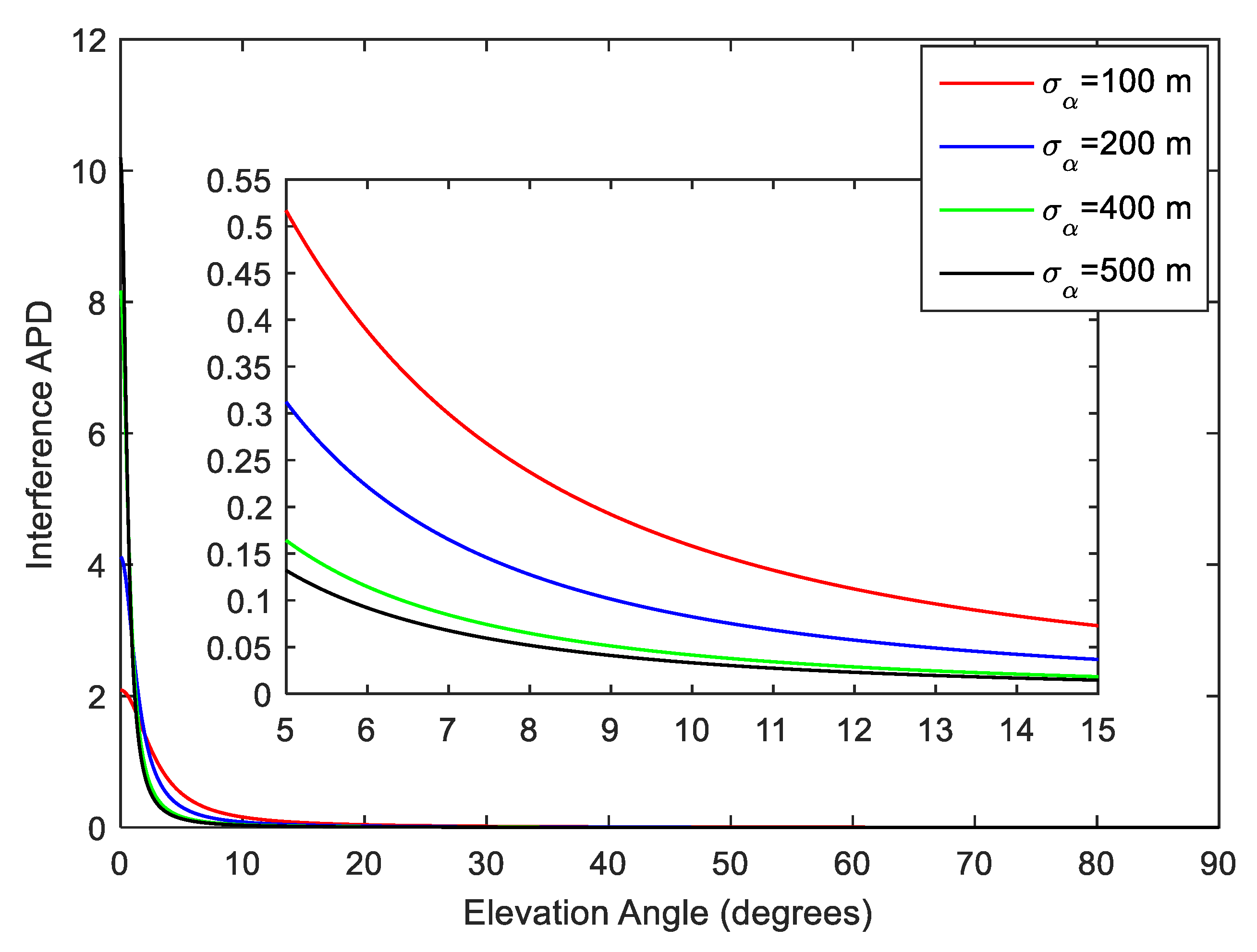
5.1. Interference APD

Figure 2 demonstrates interference APD for different standard deviations ${\sigma }_{\alpha }$ of the Gaussian distribution in the horizontal direction and an interference APD in the scenario where the incoming interference power is assumed to obey the uniform distribution in the 3D space. In the actual urban C-V2X communication, the effective interferer’s height is limited, but it may be far from the receiver ${\mathrm{R}}_{\mathrm{X}}$ in the horizontal direction. Therefore, the horizontal interference has a greater influence on the statistical characteristics of the interference, and Figure 2 only considers the impact of different ${\sigma }_{\alpha }$. In the above equations, the unit of the elevation angle is radians. For ease of description and understanding, the unit of the elevation angle in all simulations in Section 5 is degrees, so the interference APD in Figure 2 has some values greater than 1. If the incoming interference power is assumed to obey the uniform distribution in the 3D space, the interference APD can be derived as $\cos \beta /2\pi$. As shown in Figure 2, the larger ${\sigma }_{\alpha }$ is, the more interference power is concentrated in the small elevation angle range. When ${\sigma }_{\alpha }\ge 400 \mathrm{m}$, the interference APD curves tend to coincide. According to the $3\sigma$ principle of the Gaussian distribution, this indicates that the interference effects outside the horizontal distance $3{\sigma }_{\alpha }\ge 1200 \mathrm{m}$ are small due to the large path loss and shadow fading. For different ${\sigma }_{\alpha }$, the interference APD curves decrease sharply with the increase of the elevation angle. When the elevation angle is 15°, the interference APD values are 0.072, 0.037, 0.018, and 0.014, respectively; that is, the curves are almost reduced to zero. The interference APD curve under the assumption of uniform distribution decreases extremely slowly with the increase of the elevation angle, which cannot well characterize the law that the influence of the interference in the vertical direction is small in the actual C-V2X communication. The above spatial statistics of interference can provide reference for the design of the antenna arrays and the beamforming technology, so that the antenna and the beam avoid the main interference to improve the C-V2X communication performance.

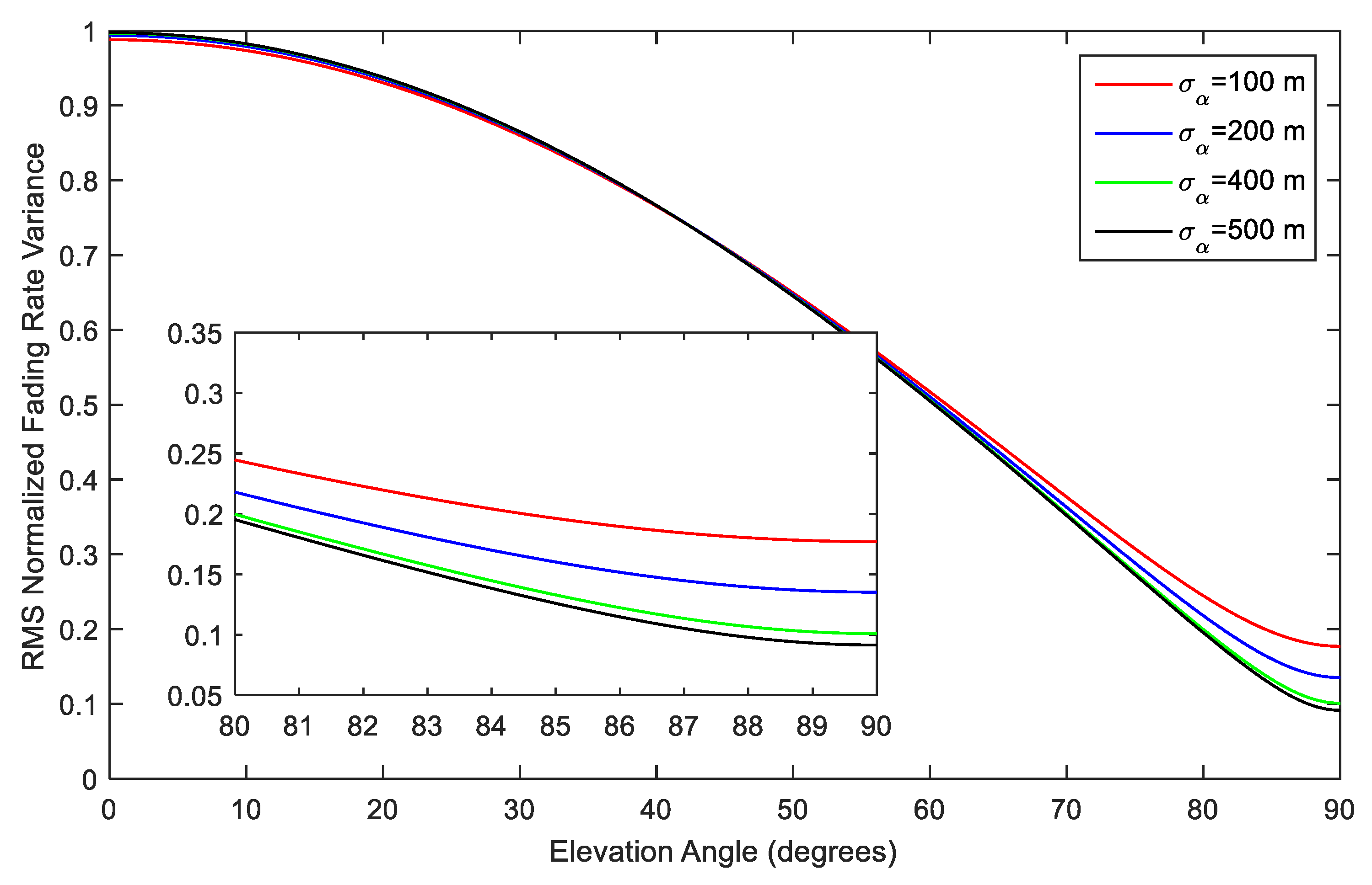
5.2. Interference Fading Rate Variance

Figure 3 demonstrates the root-mean square (RMS) normalized fading rate variance of interference for different ${\sigma }_{\alpha }$ and elevation angles. For facilitating comparison with the 2D GIDM, Figure 3 uses the RMS normalized fading rate variance, which is the root-mean square of the “3D fading rate variance/2D fading rate variance”. The 2D fading rate variance can be derived as ${\sigma }_{I_{2D}}^2=2{\pi }^2{P}_I/{\lambda }^2$. As shown in Figure 3, as ${\sigma }_{\alpha }$ increases, the RMS normalized fading rate variance curves almost coincide in the range of (0°, 60°) of elevation. The curves differ in the range of (60°, 90°) of elevation, and moreover, the larger ${\sigma }_{\alpha }$ is, the smaller the RMS normalized fading rate variance is at the same elevation angle, but when ${\sigma }_{\alpha }\ge 400 \mathrm{m}$, the curves tend to be consistent. For example, the average relative deviation of RMS normalized fading rate variances at ${\sigma }_{\alpha }=400 \mathrm{m}$ and ${\sigma }_{\alpha }=500 \mathrm{m}$ has been reduced to 0.8%, which also shows that the interference effects outside the horizontal distance $3{\sigma }_{\alpha }\ge 1200 \mathrm{m}$ are small. The RMS normalized fading rate variance in Figure 3 is less than or equal to one, which indicates that the received interference power fades slower for 3D GIDM than 2D GIDM. For wireless communication, the smaller interference, and the higher fading speed of interference are good for improving system performance. As shown in Figure 2 and Figure 3, the interference APD is almost zero and the RMS normalized fading rate variances are large near the elevation angle of 15°. Therefore, the elevation angle of 15° is the proper direction of antenna and beam pointing.

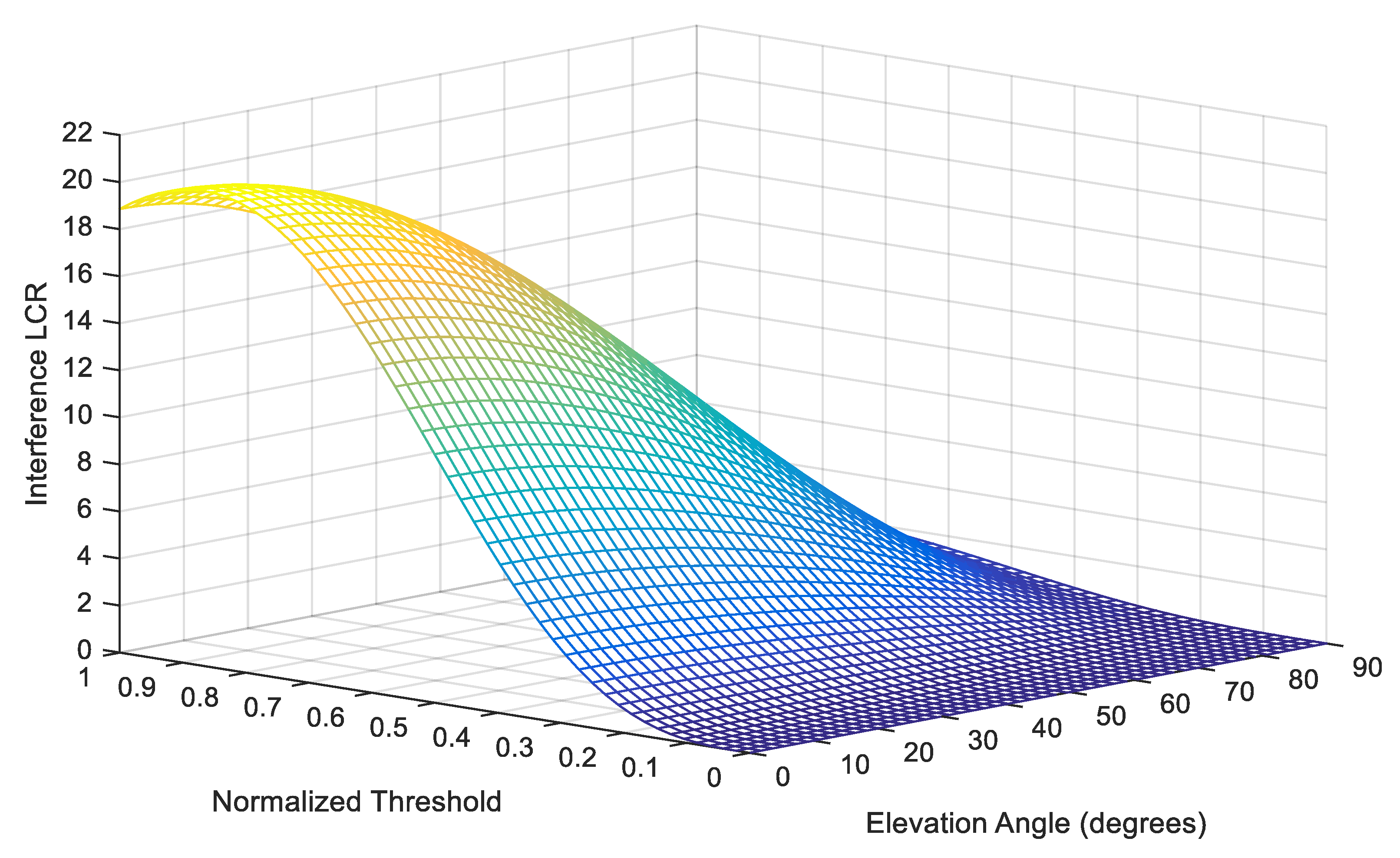
5.3. Interference LCR

Figure 4 demonstrates the interference LCR for different normalized thresholds and elevation angles. As shown in Figure 4, the normalized threshold has a decisive effect on the interference LCR, and the elevation angle also has a significant effect on the interference LCR. As the normalized threshold increases, the interference LCR also increases rapidly. As the elevation angle increases, the interference LCR gradually decreases. When the elevation angle approaches 90°, the interference LCR decreases to almost zero, indicating that the interference fading speed becomes slower and the fluctuation also becomes smaller when approaching the vertical direction, and Figure 3 also reflects this characteristic of interference. According to Equation (21), the interference AFD is inversely proportional to the interference LCR at the same normalized interference threshold. Therefore, the variation law of the interference AFD for different normalized thresholds and elevation angles can also be obtained from Figure 4.

5.4. Interference SCF

Figure 5 demonstrates the interference SCF for different spatial distances and elevation angles and whether the spatial distance or the elevation angle has a decisive effect on the interference SCF. In the range of (0°, 60°) of elevation, the effect of the spatial distance is dominant, and when the spatial distance is $r_c\ge 0.5\lambda$, the interference SCF approaches zero. However, in the range of (60°, 90°) of elevation, the effect of the elevation angle is dominant, and when the elevation angle approaches 90°, even if the spatial distance is $r_c=\lambda$, the interference SCF is still large. The SCF is an important indicator to measure the spatial selectivity of interference, which can guide the optimal design of the separation distance of antenna arrays. According to Figure 5, the separation distance of antenna arrays should be changed with the change of the elevation angle, that is, a small separation distance is required at low elevation angles to reduce the influence of interference correlation, and a large separation distance is required at high elevation angles. Similarly, the interference SCF is almost close to zero when $r_c\ge 0.25\lambda$ near the elevation angle of 15°.

5.5. PDF of SIR

Figure 6 demonstrates the PDF of SIR for different Nakagami-m shape factor m and the Rice K-factor K. According to the Shannon formula, the channel capacity mainly depends on the SIR, which is an important indicator for measuring channel quality. Large-capacity transmission requires a high SIR. Since this paper mainly studies the variation of interference and SIR, regardless of the specific amplitude, the average power of the interference signal and the useful signal is set to $P_I=P_S=1$. Therefore, the peaks of the PDF curves in Figure 6 are around 0 dB, and the peak position moves slightly with the change of m and K. The larger the K is, the smaller the overall fluctuation and attenuation of the multipath signal. Similarly, the larger the m is, the smaller the overall fluctuation and attenuation of the total interference at the receiver. As shown in Figure 6, the PDF of SIR is directly affected by m and K. The larger the m or K is, the more concentrated the PDF curve is, and the closer the peaks of the PDF curves are to the 0 dB. Moreover, the effects of m and K have a superposition effect.

5.6. SCF of SIR

Figure 7 demonstrates the SCF of SIR for different azimuth angles, elevation angles, and spatial distances. Since Equation (43) requires $a_2={\left(K+1\right)}^2/\left(2K+1\right)>2$, this section sets $K=4$. In addition, the azimuth and elevation angles of the LoS path of the useful signal are set to ${\alpha }_0=\pi /4$ and ${\beta }_0=\pi /6$, respectively. As shown in Figure 7, the separation distance or the elevation angle has a decisive effect on the SCF of SIR, while the azimuth angle has less of an effect. When the separation distance ${\eta }_c<0.1\lambda$, the SCF of SIR is small, and it is basically not affected by the 3D direction. As the separation distance increases, the SCF of SIR also increases, which indicates that the SCF of the useful signal decays more slowly than the SCF of the interference signal. The SCF of SIR is large in the range of (0°, 60°) of elevation angle, however, it is small in the range of (60°, 90°) of elevation angle, which indicates that the SCFs of the useful signal and the interference signal also have different fading speeds in different ranges of elevation angle. Figure 6 and Figure 7 describe the variation of the spatial statistics of SIR in the 3D space, which provides theoretical support for the design and performance evaluation of the large-capacity C-V2X transmission technology.

6. Conclusions

In this paper, a 3D GIDM has been proposed to analyze the spatial characteristics of C-V2X communication interference in the angular domain. Then, the closed-form expressions of interference APD, some key spatial statistics of interference, PDF, and SCF of SIR have been derived based on the 3D multipath shape factors theory and spatial statistics of the Rice channel. The interference APD and the key spatial statistics of interference can well characterize the different strengths of co-channel interference of C-V2X communication in different 3D angular directions. Simulation analysis shows that 3D spatial angular directions have a significant effect on these spatial statistics of interference and the SCF of SIR. The results provide useful insight on the design and performance evaluation of the large-capacity transmission technology for the interference- limited networks. In future research, the following work will be very important: (1) the frequency reuse, channel access, and modulation can also deeply affect the performance of C-V2X communication interference and these factors need to be considered in further researches; (2) the difference between 3D model and 2D model of interference in a quantitative manner needs to be investigated by actual signal measurements.

References

1. Du, D.; Zeng, X.; Jian, X.; Yang, F.; Sun, M. 3-D V2V MIMO Channel Modeling in Different Roadway Scenarios with Moving Scatterers. Prog. Electromagn. Res. 2018, 64, 43–54. [Google Scholar]
2. Taranetz, M.; Rupp, M. A circular interference model for heterogeneous cellular networks. IEEE Trans. Wirel. Commun. 2016, 15, 1432–1444. [Google Scholar] [CrossRef]
3. Zhang, T.; Lu, A.; Chen, Y.; Chai, K.K. Aggregate interference statistical modeling and user outage analysis of heterogeneous cellular networks. In Proceedings of the IEEE International Conference on Communications (ICC), Sydney, Australia, 10–14 June 2014; pp. 1260–1265. [Google Scholar]
4. Giovanidis, A.; Corrales, L.D.A.; Decreusefondf, L. Analyzing interference from static cellular cooperation using the nearest neighbour model. In Proceedings of the 13th International Symposium on Modeling and Optimization in Mobile, Ad Hoc, and Wireless Networks (WiOpt), Mumbai, India, 25–29 May 2015; pp. 576–583. [Google Scholar]
5. Koufos, K.; Jantti, R. Interference Modelling Using Hierarchical Spatial Clustering of Terrain and User Density Map. In Proceedings of the IEEE 79th Vehicular Technology Conference (VTC Spring), Seoul, Korea, 18–21 May 2014; pp. 1–5. [Google Scholar]
6. Cong, Y.; Zhou, X.; Kennedy, R.A. Interference prediction in mobile ad hoc networks with a general mobility model. IEEE Trans. Wirel. Commun. 2015, 14, 4277–4290. [Google Scholar] [CrossRef]
7. Chun, Y.J.; Hasna, M.O.; Ghrayeb, A. Modeling and analysis of HetNet interference using Poisson Cluster Processes. In Proceedings of the IEEE 25th Annual International Symposium on Personal, Indoor, and Mobile Radio Communication (PIMRC), Washington, DC, USA, 2–5 September 2014; pp. 681–686. [Google Scholar]
8. Torrisi, G.L.; Leonardi, E. Simulating the tail of the interference in a Poisson network model. IEEE Trans. Inform. Theory 2013, 59, 1773–1787. [Google Scholar] [CrossRef]
9. Huan, C.; Liu, C.; Zheng, W.; Fu, Y. Average received interference power analysis of D2D communication in the cellular network. In Proceedings of the IEEE International Conference on Ubiquitous Wireless Broadband (ICUWB), Nanjing, China, 16–19 October 2016; pp. 1–4. [Google Scholar]
10. Zhang, Y.; Zheng, J.; Lu, P.S.; Chen, S. Interference Graph Construction for Cellular D2D Communications. IEEE Trans. Veh. Technol. 2016, 66, 3293–3305. [Google Scholar] [CrossRef]
11. Li, X.; Zhang, W.; Zhang, H.; Li, W. Mathematical characteristics analysis of uplink interference region in D2D communications underlaying cellular networks. In Proceedings of the IEEE Seventh International Conference on Ubiquitous and Future Networks (ICUFN), Sapporo, Japan, 7–10 July 2015; pp. 557–561. [Google Scholar]
12. Lu, H.; Wang, Y.; Chen, Y.; Liu, K.J. Interference model and analysis on device-to-device cellular coexist networks. In Proceedings of the IEEE Global Conference on Signal and Information Processing (GlobalSIP), Orlando, FL, USA, 14–16 December 2015; pp. 1086–1090. [Google Scholar]
13. Tchouankem, H.; Lorenzen, T. Measurement-based evaluation of interference in Vehicular Ad-Hoc Networks at urban intersections. In Proceedings of the IEEE International Conference on Communication Workshop (ICCW), London, UK, 8–12 June 2015; pp. 2381–2386. [Google Scholar]
14. Bastani, S.; Landfeldt, B. The Effect of Hidden Terminal Interference on Safety-Critical Traffic in Vehicular Ad Hoc Networks. In Proceedings of the 6th ACM Symposium on Development and Analysis of Intelligent Vehicular Networks and Applications, Valletta, Malta, 13–17 November 2016; pp. 75–82. [Google Scholar]
15. Kimura, T.; Saito, H. Theoretical Interference Analysis of Inter-vehicular Communication at Intersection with Power Control. In Proceedings of the 19th ACM International Conference on Modeling, Analysis and Simulation of Wireless and Mobile Systems, Valletta, Malta, 13–17 November 2016; pp. 3–10. [Google Scholar]
16. Bithas, P.S.; Efthymoglou, G.P.; Kanatas, A.G. Intervehicular communication systems under co-channel interference and outdated channel estimates. In Proceedings of the IEEE International Conference on Communications (ICC), Kuala Lumpur, Malaysia, 23–27 May 2016; pp. 1–6. [Google Scholar]
17. Tengstrand, S.O.; Fors, K.; Stenumgaard, P.; Wiklundh, K. Jamming and interference vulnerability of IEEE 802.11 p. In Proceedings of the IEEE International Symposium on Electromagnetic Compatibility (EMC Europe), Gothenburg, Sweden, 1–4 September 2014; pp. 533–538. [Google Scholar]
18. Fuxjaeger, P.; Ruehrup, S. Validation of the NS-3 Interference Model for IEEE802. 11 Networks. In Proceedings of the IEEE 8th IFIP Wireless and Mobile Networking Conference (WMNC), Munich, Germany, 5–7 October 2015; pp. 216–222. [Google Scholar]
19. Chen, Y.; Mucchi, L.; Wang, R. Angular spectrum and second order statistics of interference in wireless networks. In Proceedings of the IEEE International Conference on Communication, Networks and Satellite (COMNETSAT), Yogyakarta, Indonesia, 3–4 December 2013; pp. 41–45. [Google Scholar]
20. Chen, Y.; Mucchi, L.; Wang, R.; Huang, K. Modeling Network Interference in the Angular Domain: Interference Azimuth Spectrum. IEEE Trans. Commun. 2014, 62, 2107–2120. [Google Scholar] [CrossRef] [Green Version]
21. Jiang, H.; Zhang, Z.; Dang, J.; Wu, L. A Novel 3D Massive MIMO Channel Model for Vehicle-to-Vehicle Communication Environments. IEEE Trans. Commun. 2018, 66, 79–90. [Google Scholar] [CrossRef]
22. Nawaz, S.J.; Qureshi, B.H.; Khan, N.M. A Generalized 3-D Scattering Model for a Macrocell Environment with a Directional Antenna at the BS. IEEE Trans. Veh. Technol. 2010, 59, 3193–3204. [Google Scholar] [CrossRef]
23. Bell, W.W. Special Functions for Scientists and Engineers; Dover Publications: New York, NY, USA, 2004. [Google Scholar]
24. Valchev, D.G.; Brady, D. Three-dimensional multipath shape factors for spatial modeling of wireless channels. IEEE Trans. Wirel. Commun. 2009, 8, 5542–5551. [Google Scholar] [CrossRef]
25. Durgin, G.D.; Rappaport, T.S. Theory of multipath shape factors for small-scale fading wireless channels. IEEE Trans. Antennas Propag. 2000, 48, 682–693. [Google Scholar] [CrossRef]
26. Nakagami, M. The m-distribution-A general formula of intensity distribution of rapid fading. In Statistical Method of Radio Propagation; Pergamon: Oxford, UK, 1960; pp. 3–36. [Google Scholar]
27. Babich, F.; Lombardi, G. General Nakagami approximation for sum of Ricean interferers. Electron. Lett. 1998, 34, 23–24. [Google Scholar] [CrossRef]
28. Papoulis, A.; Pillai, S.U. Probability, Random Variables, and Stochastic Processes; Tata McGraw-Hill Education: New York, NY, USA, 2002. [Google Scholar]
29. Karagiannidis, G.; Georgopoulos, C.; Kotsopoulos, S. Outage probability analysis for a Nakagami signal in L Nakagami interferers. Eur. Trans. Telecommun. 2001, 12, 145–150. [Google Scholar] [CrossRef]
30. Dubey, S.D. Compound gamma, beta and F distributions. Metrika 1970, 16, 27–31. [Google Scholar] [CrossRef]
31. Du, D.; Zeng, X.; Jian, X.; Yu, F.; Miao, L. Analysis of Three-Dimensional Spatial Selectivity for Rician Channel. Radioengineering 2018, 27, 249–255. [Google Scholar] [CrossRef]
Figure 1. The 3D Gaussian interference distribution model (GIDM) of interference.
Electronics 08 00718 g001
Figure 2. The interference angular power density (APD).
Electronics 08 00718 g002
Figure 3. The root-mean square normalized fading rate variance of interference.
Electronics 08 00718 g003
Figure 4. The interference level crossing rate (LCR).
Electronics 08 00718 g004
Figure 5. The interference spatial correlation function (SCF).
Electronics 08 00718 g005
Figure 6. The probability density function (PDF) of signal–to–interference ratio (SIR).
Electronics 08 00718 g006
Figure 7. The SCF of SIR.
Electronics 08 00718 g007