1. Introduction
Compared to the current fourth generation (4G) wireless networks, the fifth generation (5G) networks are expected to support massive connectivity of devices so as to satisfy the growth of internet of things. The channel multiple access schemes determine the number of users to share the wireless resources, which mainly include orthogonal multiple access (OMA) and non-orthogonal multiple access (NOMA) [
1]. It is difficult for OMA to meet the spectral efficiency requirements of 5G services. Power-domain NOMA and code-domain NOMA are two categories of NOMA schemes. For the former, multiple users are allocated with different power levels at the same time and channel frequency. Specifically, higher power is assigned to the users with worse channel gains; and lower power is allocated to the ones with better channel gains. In terms of compatibility with existing OMA schemes, power-domain NOMA is more promising.
Cooperative communication adopts relay strategies to improve system reliability, amplify-and-forward (AF) and decode-and-forward (DF) are two common types of processing protocols by the relay terminals [
2]. A prior study [
3] derived the outage probability and diversity multiplexing trade-off curve for an uplink cooperative system with DF protocol. Cooperative NOMA transmission has been proposed to enhance the overall performance of communication systems, as well as reducing the transmit power [
4]. The status of recent research in power-domain NOMA-based cooperative networks are surveyed in [
5]. In order to prolong the lifetime of energy constrained relay systems, NOMA can be integrated with simultaneous wireless information and power transfer (SWIPT) [
6,
7].
For AF relay systems, data detection at the destination only requires the information of the cascaded channel through the source-to-relay-to-destination link. Therefore, the estimation algorithms of the cascaded channel are proposed in [
8,
9]. Additionally, the statistical properties of the cascaded relay fading channels are investigated in [
10], where the cascaded channel is modeled as a double Gaussian channel, i.e., a product of two complex Gaussian channels.
There have been numerous studies that focus on the performance analysis of cooperative NOMA systems [
11,
12,
13]. One prior study [
11] derived the exact and asymptotic outage probabilities for NOMA AF systems. The authors in [
12] studied NOMA-based downlink AF relaying network under Nakagami-m fading and derived the closed-form expressions of the outage probability, with imperfect channel state information taken into account. In [
13], a two-stage relay selection scheme was proposed and a closed-form expression of the outage probability was derived. Almost all the previous literature concentrated on evaluating the outage probability. There are few reports about the error performance analysis for cooperative NOMA systems. In [
14], the error rate was analyzed in non-cooperative NOMA systems over Nakagami-m fading channels.
To the best of our knowledge, there is no closed-form solution for the pairwise error probability (PEP) expressions of NOMA users based on order statistics of the cascaded channel for relay NOMA communication systems in the literature. In this paper, we mainly analyze the PEP performance of NOMA systems with multiple AF relay–user pairs. Our specific contributions of this paper are summarized as follows:
We derive the approximate closed-form PEP expressions of the first and the kth users over Rayleigh fading channels, respectively. In particular, the ordered probability density function (PDF) of the cascaded channel is utilized to solve the integrals. Simulation results reveal the consistency between the derived closed-form PEP expressions and their corresponding Monte Carlo simulations.
We attempt to substitute
, namely, the
pth power of modified Bessel function
, with an approximately equivalent finite series representation since the presence of the power of the modified Bessel function of the second kind,
, makes the integrals about the PEP of NOMA users intractable. In existing literature, there is no appropriate finite series representation of
. Therefore, we derive an effective and simplified series representation of
based on the series representation of
in [
15]. The major difficulty lies in that a smaller
x value will result in a significant truncation error between the approximated
and the actual
once the choice of the finite order is improper. To some extent, the effectiveness of the derived closed-form PEP expression is dependent on the accurate representation of finite series of
.
The impacts of some related parameters, such as power allocation coefficients of NOMA users and power splitting factor related to energy harvesting, can be evaluated through the simulations by using the approximate closed-form PEP expressions.
The rest of the paper is organized as follows. First, the system model is given in
Section 2 for the considered cooperative NOMA system. The analytical PEP expression of the first user is derived in
Section 3. In
Section 4, we present the approximate finite series representation of
. The closed-form PEP of the
kth successive interference cancellation (SIC) useris derived in
Section 5. The numerical and simulation results are provided for analytical confirmation in
Section 6. Finally, the paper is concluded in
Section 7.
2. System Model
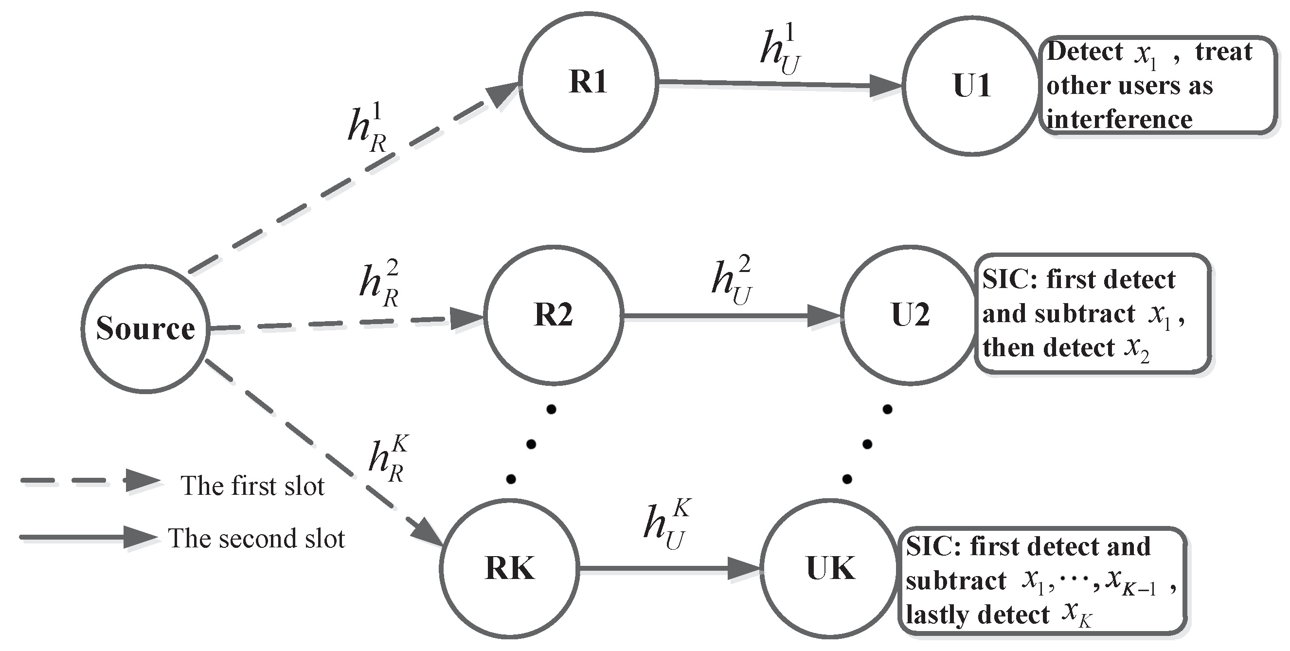
We consider a downlink relay NOMA system with K users assisted by K relays as depicted in
Figure 1, where all are equipped with a single antenna. NOMA technique enables various users to manipulate individual information under the conditions of identical time and frequency resources. The base station (BS) broadcasts the superimposed information to K users with the help of respective relays, which are equipped with the function of simultaneous wireless information and power transfer (SWIPT). We adopt a half-duplex amplify-and-forward (AF) relay with no direct link due to severe obstruction or shadow. Considering energy harvesting, the power splitter (PS) scheme at the relay is adopted, which can split the receiver signal power into two parts comprising of energy harvesting and information processing [
16].
At the BS with known power allocation coefficient
of the
kth user, the superimposition signal of NOMA users is transmitted, which is denoted as
where
is the total power at the BS.
is the data symbol of the
kth user. Moreover,
and
.
The users accomplish signal reception through two time slots. In the first time slot, BS broadcasts the signal to the relay, thus the received signal at the relay is
where
represents the channel coefficients from the source to relay.
indicates the additive white Gaussian noise at the relay.
After power splitting at the relay, the signals about energy harvesting and information forwarding are written as, respectively
where
is a PS factor, and
is the conversion noise from RF to baseband.
In the second time slot, with the relay operating the AF protocol and forwarding the information signal, the received signal of the
kth user can be written as
where
, and
represents the channel coefficients from the relay to users. Moreover,
is the additive white Gaussian noise at the destination. Assume
and
. It can be observed that the knowledge of individual channels
and
is not required for data detection. As a result, the cascade channel
is considered in the following analysis. The amplification factor
is denoted as
where
is the harvested power at the relay in the second time slot.
denotes energy conversion efficiency.
Considering the fixed-gain amplification factor,
can be rewritten as
For each receiver, successive interference cancellation (SIC) is utilized to remove the interference and implement the accurate signal detection. Specifically, for the kth user, the manipulation of SIC is to successively detect the signals and subtract them from the received signal. The signals of the remaining users are treated as interference.
3. PEP Derivation of the First User
The SIC process is not required for the first user. Plugging (
1) into (
5), the received signal of the first user can be formulated as
where
is viewed as the interference component during the process of detecting the first user. The conditional pairwise error probability (PEP) of the first user can be expressed as
where
denotes the event in which
is erroneously detected into the symbol
.
Inserting (
8) into (
9), (
9) can be rewritten as
where
,
. Moreover,
, which further turns Equation (
10) into
where
is the amplitude of the cascaded channel.
denotes the Q-function.
and
are given by
Without taking the instantaneous channel into account,
can be further written as
Generally, the ordered PDF of the cascaded channel
regarding the
kth user is represented as [
17]
where
and
represent the PDF and cumulative distribution function (CDF) of
, and
Assume that all the separate channels undergo Rayleigh fading, which means
is the amplitude of the product of two complex Gaussian random variables [
18], so the PDF and CDF of
are expressed as
where
and
are the modified Bessel function of the second kind with zero order and first order, respectively.
Consequently, with
assumed, the ordered PDF of the first user is given by
It follows that the exact PEP of the first user is solved as
where
,
.
Proposition 1. The approximate closed-form PEP of the first user can be represented aswhere is the gamma function, denotes a parabolic Cylinder function, and Proof of Proposition 1. Equation (
20) can be further formulated as
In (
23),
is replaced by
. It can be easily derived that
. Moreover, the first term on the right side of the third equal sign can be computed as
In the above limit derivations, we exploit the asymptotic expressions of
, namely
when
, while
when
[
19].
Therefore, based on Equation (
34) in
Section 4,
can be further expressed as
where
is given by (
22) in the next section. It is worth noting that
can be stored as a vector with constants in advance.
Subsequently, plugging (
26) into (
23) yields
where the last equation is obtained according to ([
20], Equation (3.462.1)). □
4. Approximate Finite Series Representation of
In order to facilitate the integral in (
23), it is essential to explore the equivalent series representation of
. According to [
15] (Equation (
24)), the series representation of
can be given by
with the coefficients being
where
denotes the Lah numbers ([
15], Equation (
8)), namely,
, for
. The other values can be taken as:
; for
,
and
. Let
, (
28) can be simplified by
Hence, it is straightforward to obtain the
pth power of
as
Utilizing the mathematical operation regarding power series raised to powers [
21], the power of
can be further converted into
where
with
,
.
From the perspective of practical implementation, it is normal to consider the approximate representation in terms of finite series terms of the Bessel function
[
15]. However, there is no existing work about the finite series representation of
. In the following, we will examine whether
can be truncated by only using a small series order with high precision instead of infinite series in (
32).
It is apparent that there exist two infinity series in the expression of
in Equation (
32). The outer series can be approximated by the finite order
Q, namely,
where
indicates the truncation error, which is negligible with a small
Q, as illustrated in
Table 1. Moreover, the smaller Q is, the less coefficients are required to store. The series
within the coefficient
is truncated by the parameter
, namely,
where
and
Q are positive integers,
, and
[
15].
Remark 1. It is worth noting that two identical finite orders are chosen to replace two infinity series about in [15] (Equation (24)). Unlike that, we attempt to exploit two different finite orders to truncate the infinite series of , which can improve the accuracy when . Apparently, the former can be regarded as our special case. Remark 2. It is likely for Q and to take different values for different p in order to minimize the truncation error. We need to search for proper values about Q and for each p. Once these parameters are fixed, the coefficients can be stored in advance as shown in Table 2. The accuracy of series approximation of
exerts a direct impact on the analytical PEP derivation. We define the normalized truncation errors as
in the simulation, where the true
is generated by MATLAB command "besselk", and
. In
Table 1, take discrete values on
for example, where
is the adopted sample interval. From
Table 1, we observe that the case with
and
has the least truncation error for
. In addition,
with
is better than
for
whereas
exhibits the smaller truncation error with
than the case
for
.
For specific
,
can be generated in advance given
and
Q, as shown in
Table 2. It is worth noting that the coefficients
and
in the cases
and
are identical to the corresponding
and
with the case
, hence, the former cases are not shown in this table. Moreover,
Table 2 also illustrates
in (
34) with
and
has completely the same coefficients as
listed in [
15] (
Table 1). In any case, it is noticed that
=1 remains invariant.
5. PEP Derivation of the th SIC User
From the second user to the last user, the SIC is performed by each user. During each SIC process, the output of the
kth user is
where
is the interference cancellation error of the previously detected signal
.
After the same manipulation as above, the conditional PEP of the
kth user is given by
where
,
and
are represented as
where
. It is worth highlighting that since all previous user symbols have been detected,
for the last user is given by
where
is zero if the perfect SIC is taken into account.
From (
19), the ordered PDF of the
kth user is
Taking advantage of binomial expansion, we have
Then (
41) can be rewritten as
where
.
With
assumed, it turns out from (
43)
Therefore, the exact PEP of the
kth user can be given by
where
.
Proposition 2. The approximate closed-form PEP of the kth user can be derived aswhere , and Proof of Proposition 2. The integral term in Equation (
45) can be derived as
Therefore, the exact PEP expression can be obtained as
The above closed-form expression has a similar manipulation process to (
23). It should be pointed out that the approximate series representation of
is given by
with the coefficients
manifested in (
47). By plugging (
50) into (
48), we have
Consequently, inserting (
51) into (
45) yields
where
. Moreover, leveraging on [
20] (Equation 0.160), the summation terms in
can be rewritten as
Combined with the key property of Beta function
[
22], it follows that
□
The proof of (
46) is completed.
6. Simulation Results
This section validates the derived PEP expressions in the preceding sections. Consider a two-user NOMA SWIPT system over Rayleigh flat fading channels. BPSK modulation is adopted. The channel variance is assumed to be . In addition, other parameters are fixed as , , and , unless otherwise specified. The simulated curves are conducted through Monte Carlo simulations.
It should be pointed out that the aforementioned parabolic Cylinder function
([
20], Equation (9.240)) can be converted into
where W(·) is the Whittaker function, which is available in MATLAB toolbox.
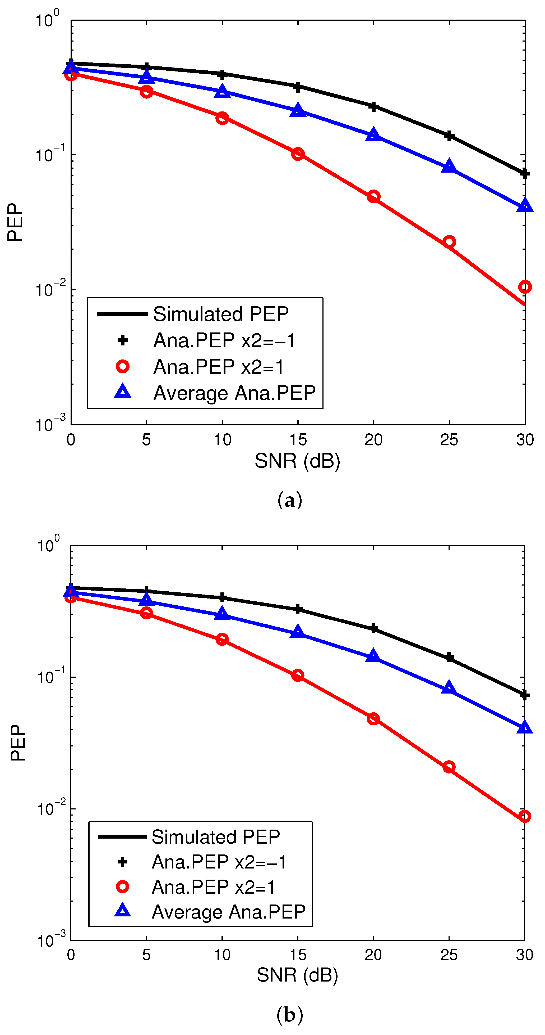
In
Figure 2, we evaluate the derived closed-form PEP (
21) for the first user compared with the simulated PEP. It is worth pointing out that the PEP of the first user is associated with
when
is fixed. The solid lines represent the simulated PEP, while the markers denote the analytical PEP. The average analytical PEP is obtained by taking the average of both cases
. As seen in
Figure 2a,b, the accuracy of the closed-formed PEP is related to the value
. When
, the analytical PEP with
is evidently inconsistent with the simulated PEP at SNR = 30 dB, which is due to the approximation error of finite series representation of
. However, the analytical PEP almost agrees well with the simulated PEP when
.
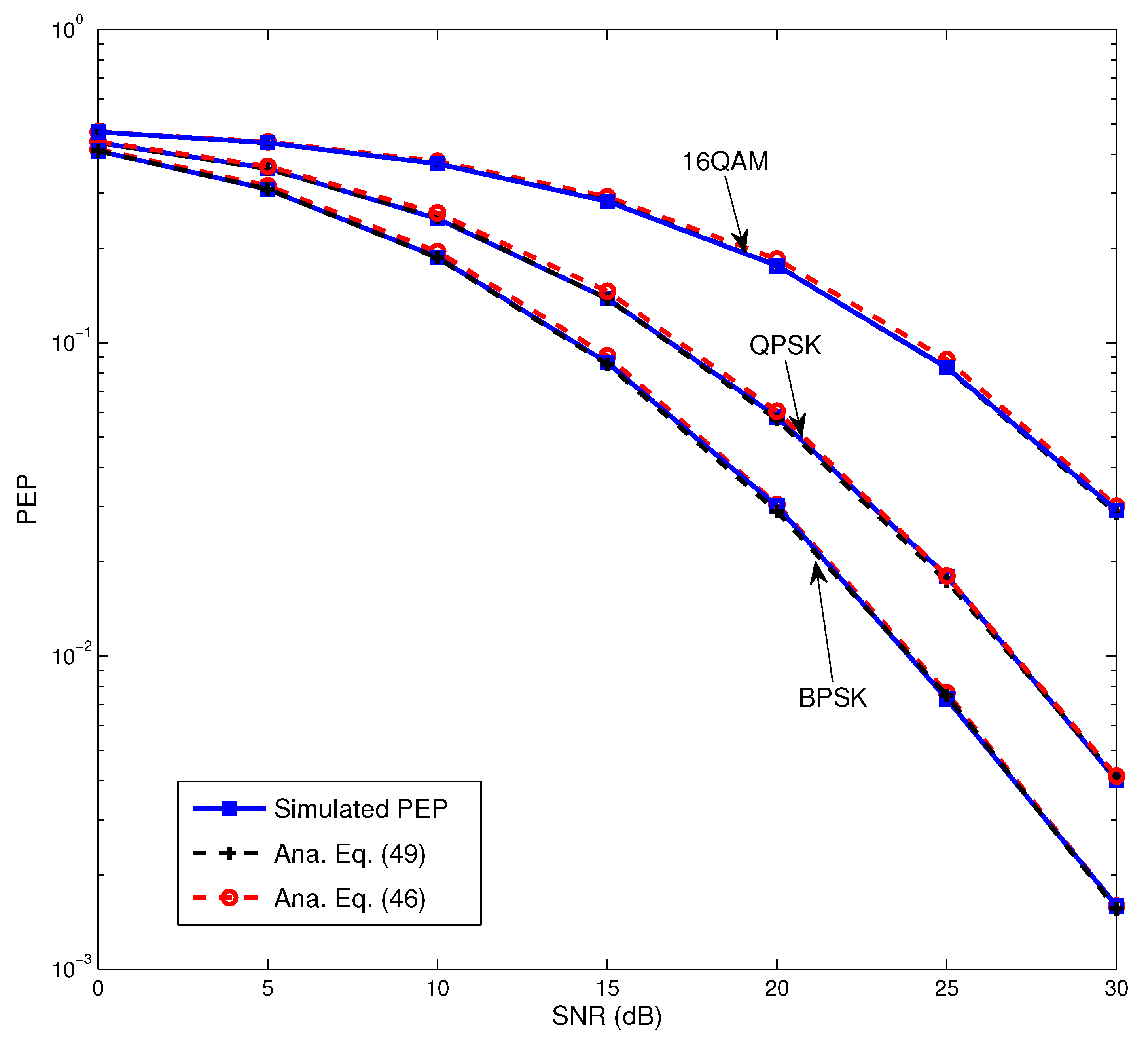
Figure 3 verifies the accuracy of the derived analytical closed-form PEP expression for the second user. Whichever modulation is adopted, the closed-form expression (
46) in Proposition 2 is consistent with the simulated PEP acquired by random Monte Carlo simulation over Rayleigh fading channels. To preclude the influence of the approximate error of finite series representation of
, (
49) is provided for more reliable reference. Specifically, for (
49), we use the existing MATLAB “Besselk” function to implement
as a benchmark. As anticipated, the simulated PEP and the analytical in Equation (
49) completely overlap. Meanwhile, Equation (
46) Proposition 2 is totally in agreement with the other two curves when
.
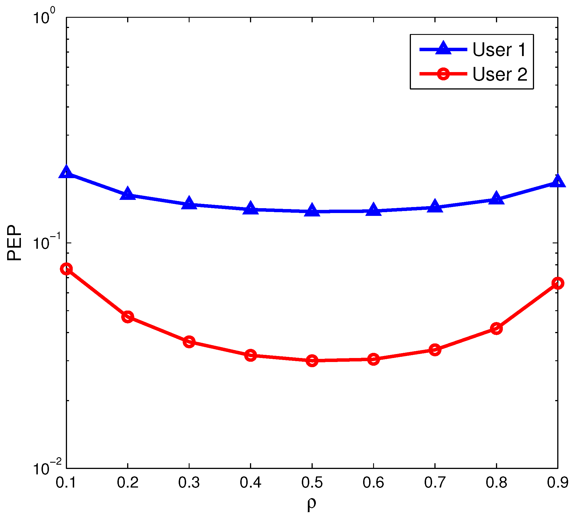
The impact of several parameter values on PEP is straightforwardly presented. The following three figures are simulated at SNR = 20 dB, and the average analytical PEP is evaluated for the first user. First, we observe the performance of PEP with varying PS factors
for two users as seen in
Figure 4. Fortunately,
= 0.5 or 0.6 simultaneously corresponds to the optimal performance of two users.
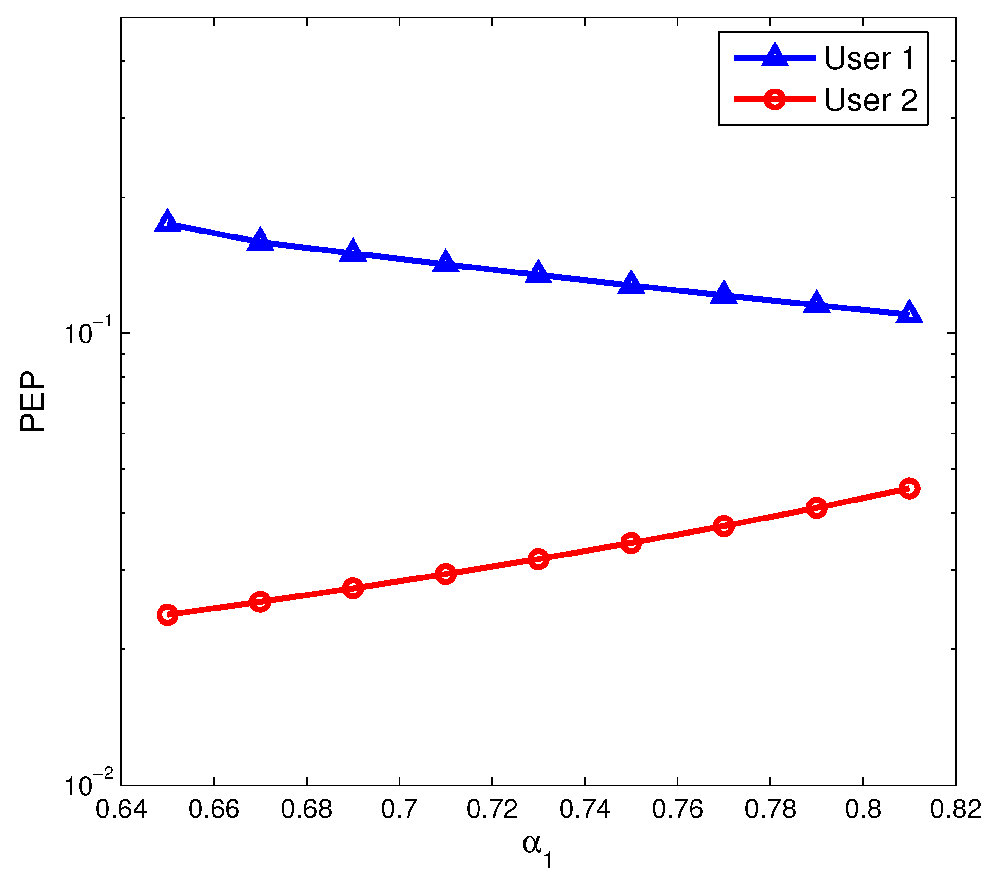
In order to evaluate the effect of power allocation coefficients, we alter
of the first user. For the second user, its power allocation coefficient will make a corresponding change due to
. As depicted in
Figure 5, the first user with a weaker channel condition performs gradually better as
slowly increases. On the other hand, the second user with stronger channel quality becomes worse due to its reduced
. The choice of power allocation coefficient depends on the required quality of service for different users.
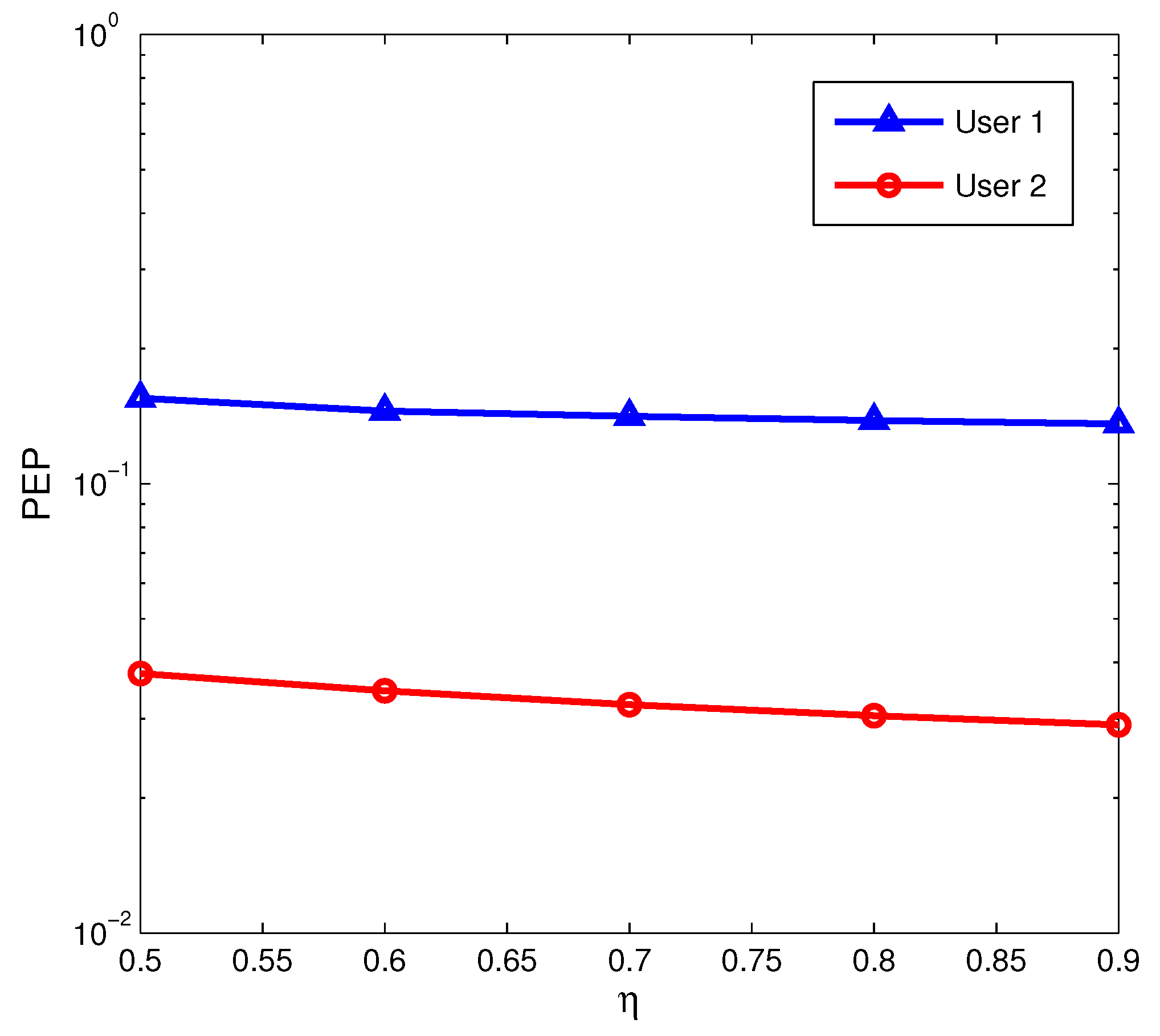
The effect of energy conversion efficiency on the error performance is explored as shown in
Figure 6. For any user, only a slight change in PEP happens when
varies from 0.5 to 0.9.
7. Conclusions
An approximate closed-form PEP analysis is derived for cooperative NOMA SWIPT systems over Rayleigh fading channels. Based on the ordered statistics of the composite channel across the Source-Relay-User link, the PDF and CDF of
are related to the modified Bessel functions of the second kind, which renders the PEP analysis very challenging. In order to obtain the closed-form PEP, the finite series representation of
is introduced. We verify the effectiveness of the approximately analytical PEP for NOMA users, which is expressed by finite series representation. Numerical results substantiate that our method agrees well with Monte Carlo simulations. It is worth pointing out that for more than three users, it needs some time to search the suitable pairs of
to match the finite series representation of
. Specifically, assuming K = k = 3, the accuracy of PEP calculations for the third user depends on the joint precision of finite series approximations of
,
, and
, which can be seen from Equation (
49). Our future work will explore an effective approach to determine the joint pairs of
for different
to adapt more users.


