Urban Crowd Detection Using SOM, DBSCAN and LBSN Data Entropy: A Twitter Experiment in New York and Madrid

Abstract

The surfer and the physical location are two important concepts associated with each other in the social network-based localization service. This work consists of studying urban behavior based on location-based social networks (LBSN) data; we focus especially on the detection of abnormal events. The proposed crowd detection system uses the geolocated social network provided by the Twitter application programming interface (API) to automatically detect the abnormal events. The methodology we propose consists of using an unsupervised competitive learning algorithm (self-organizing map (SOM)) and a density-based clustering method (density-based spatial clustering of applications with noise (DBCSAN)) to identify and detect crowds. The second stage is to build the entropy model to determine whether the detected crowds fit into the daily pattern with reference to a spatio-temporal entropy model, or whether they should be considered as evidence that something unusual occurs in the city because of their number, size, location and time of day. To detect an abnormal event in the city, it is sufficient to determine the real entropy model and to compare it with the reference model. For the normal day, the reference model is constructed offline for each time interval. The obtained results confirm the effectiveness of our method used in the first stage (SOM and DBSCAN stage) to detect and identify clusters dynamically, and imitating human activity. These findings also clearly confirm the detection of special days in New York City (NYC), which proves the performance of our proposed model.

1. Introduction

Since the advent of smartphones, the activity on social networks has become increasingly important. Our pace of activity is increasing and the consequences of this intensive lifestyle will be interesting to see. We are constantly connected; smartphones have definitely changed the way we live. How many parties have you had where there are four or five people (or more) hanging on their phones? We are always connected. This huge smartphone revolution, coupled with the large number of social network users, has unearthed a new type of service in the field of localization, known as location-based social network (LBSN) services. These are applications available on mobile devices via the mobile network that use the geographic location of the device. With the massive development of smartphones, the daily data produced is now almost systematically linked to geographical coordinates (i.e., latitude and longitude). We can cite the example of Flickr [1], whose users can upload locally tagged photos to a social networking service, the example of Foursquare [2], which allows organizations to share their current location on a website to organize an activity in the real world, and the example of Twitter, which allows Internet users to comment on an event in real time and at the exact location where it takes place. In particular, the exploitation of the large amount of information provided by Twitter, with more than 350 million users (currently in 2018), can potentially open new perspectives on the urban structure and the urban mobility process (grouping, trajectories, etc.). An LBSN does not only mean sharing our physical position with our friends, but also reflects an urban structure composed of individuals resulting from their physical location. Location information collected over time can really characterize the urban prevalence (crowd spread), spatial distribution at different moments of the urban prevalence, and detection of a grouping and monitoring of its evolution (spatial movement taking into account temporal aspects). These geolocated data are produced in huge quantity, especially from social networks such as Facebook and Twitter. The expression "big geosocial data" [3] is that by which we mean all these data. They should not be confused with the "voluntary geographic information" (VGI) of [4] as they are precisely characterized by their non-contributory nature. Indeed, since the system of "check-in" (i.e., associating a physical place with a publication) appeared with the emergence of geolocated social networks, the social sharing of geographical localization across social web platforms has become commonplace [5]. Like [6], we prefer to use the term "ambient geospatial information" rather than VGI. In a societal context where the improvement of urban intelligence is crucial, we argue that the potential offered by the analysis of geosocial data sets is an opportunity that should be seized. More precisely, we focus here on urban crowd detection and ask the following starting question: Can we use massive geosocial data to identify urban crowds using big geosocial data?

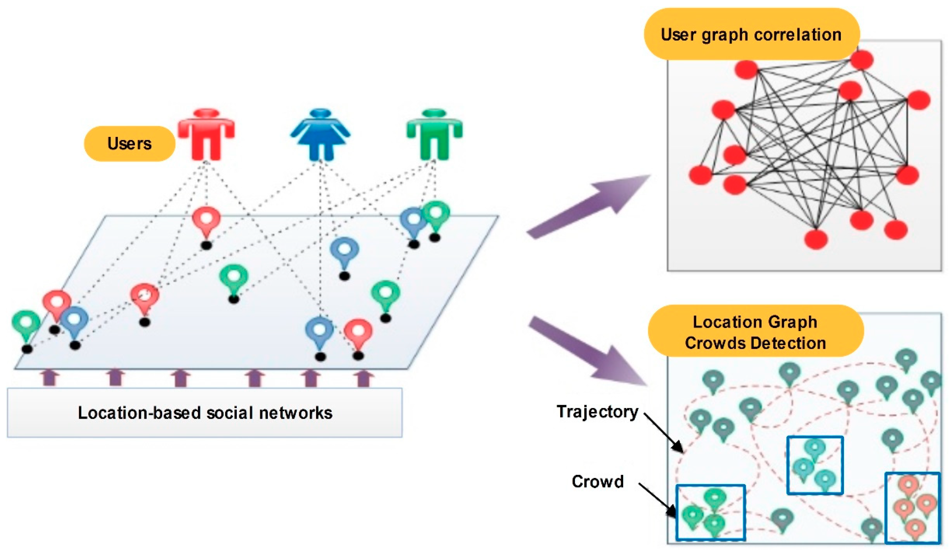
1.1. Concepts and Definitions of LBSNs

Social networks that include geolocation information in shared content are called social location networks. They provide geographical information on a map by physical proximity (real location), unlike the concept in chronological order [7]. The emergence of smartphones, equipped with sensors, allowing users to locate themselves in a sustainable way and at any place in urban areas, has offered a major development potential in this field. location-based services (LBS) technologies are behind this geolocation. They allow you to customize the content of a mobile device based on its location. These are application services that use the location data of mobile terminals to provide them with personalized content and applications, depending on their geographical position. This type of service can be used in a very wide variety of fields: Marketing, advertising, health, work, etc.

LBS can be applied to both a fixed object (typically a point of interest) and a moving object. In the second case, it will generally be another terminal. With the development of smartphones, LBS can increasingly integrate geolocation data as a search criterion. A set of elements that will allow personal assistants, such as Siri (from Apple) or Cortana (from Microsoft), to offer a personalized search for each user integrating this geolocation dimension. The applications, providing these services can be grouped into three classes: geo-tagging, point location and trajectory-based.

The user and the physical location are two important concepts that are associated with each other in the social network-based localization service. In the following, we focus on the research philosophy for urban cluster detection based on LBSNs.

1.2. Background on Crowd Detection based LBSNs

Throughout the day, we visit several physical locations and we generate a “location history”, through the rental tags. Figure 1 illustrates the relationship between the user and the history of his physical location. The sequential connection of these locations in terms of time allows us to have a trajectory for each user. The collection of positions allows us to detect urban groupings in a given region at different times. In this sense, several studies focus on the study of the behaviour and the human mobility to know the citizen movement and the detection of abnormal groups based on LBSNs.

Geolocation is one of the most common issues in LBSNs, which is made possible by various services. For these services, the user’s location is only planned with a certain precision, especially if it concerns the prediction at any time. Geolocated data are used in the follow-up study of people, usually in the context of the use of a particular space (urban space, station, etc.).

2. Related Work

Many research studies have investigated the value of using spatialized (distance and position) information to answer various questions, such as the evaluation of city activity [8,9,10], the analysis of spatial mobility [11,12,13], the epidemiology [14,15], the natural crisis management [16], and the spatial planning [17]. For more details on the proposed methods, in the context of the human mobility, the reader is invited to read in particular [18]. Noulaset [19] quantitatively analyzed a colossal mass of data from Foursquare: about 12 million check-ins were collected from geotagged tweets for a total of 679,000 users and a 100-day collection period. The results of Noulaset make it possible to conclude that the Foursquare data are representative of the daily movements of the users. Among the most relevant spatial analyses carried out on Foursquare data, we also mention Kelley’s research [20]. Ben Khalifa [21] suggested an analysis of geolocated social media data to identify urban crowds in New York City. “This analysis is gathered under a methodology for crowd detection in cities that combines social data mining, density-based clustering and outlier detection into a solution that can operate on-the-fly” According to Gao [22], the availability of big geo-social data on LBSNs provides an unheated opportunity to “study human mobile behavior through data analysis in a spatial-temporal-social context, enabling a variety of LBS, from mobile marketing to disaster relief”. With the development and speedy admiration of LBSN, Domíngueza [23] proposed a system for the detection of abnormal high or low number of citizens in a given area on the basis of these services. Pelechrinis [24] presented practices and methods in the field of urban computing as well as open challenges; civic data and technologies for urban detection, analytical techniques used for urban data analysis and concrete examples of urban computing applications. In [25], the authors showed that location-based social media systems such as Instagram and Foursquare can serve as valuable sources of large-scale detection, and provide access to important characteristics of urban social behavior much faster than traditional methods. In [26], the authors studied human activity from mobile socio-demographic data in six Italian cities. Roberts [27] proposed the use of Twitter data for urban green space research. Time and geo-coordinates associated with a sequence of messages or tweets reflect the spatial and temporal movements of people in real life. The purpose of the Comito research [28] was to analyze these movements in order to discover community behaviors and to determine popular travel routes from geo-tagged stations (i.e., collected geo-tagged data). Kanno [29] “proposed a method that measures demographic snapshots of a city from time- and geo-stamped micro-blog posts and visualizes high-risk evacuation roads on the basis of geographical characteristics and demographics”. According to the author, this method allows a high level of situational awareness (hourly) to be achieved in order to provide evacuation routes. Kim [30] “proposed a new system of analyzing the spatiotemporal patterns of social phenomena in real time and the discovery of local topics based on their latent spatiotemporal relationships”. Yang et al. [31] presented an observational study of the geolocated activities of the users on two social media platforms, performed over a period of three weeks in four European cities. This study showed how demographic, geographical, technological and contextual properties of social media (and their users) can provide very different reflections and interpretations of the reality of an urban environment. The work of Bordogana [32] exploited the timestamped geo-labelled messages posted by Twitter users from their smartphones when they travel to track their journeys. To learn more about how social media data can be used to infer knowledge about urban dynamics and mobility patterns in an urban area, the reader is invited to read [33]. In [34], two types of data were used to determine the user communities. The authors studied the use of the physical space through the individual data (to track movements) and the overall use of the space. Ahas [35] pointed out that the main shortcomings of the telephone data are the difficulty of accessing the data and the lack of precision of the locations, where the considered location is most often that of the antenna to which the telephone is connected. We can also cite several types of geolocated data of interest by using the classification of Senaratne [36].

In this work, we use geolocated social data provided by the Twitter API to detect and identify an urban grouping. Successful grouping identification relies on two different techniques: the Kohonen topological maps [37,38] based on unsupervised learning methods and DBSCAN [39].

3. Methodology

The proposed methodology, for urban crowd detection, consists of three phases: using the SOM to map the input space and select the DBSCAN parameters, applying the DBSCAN algorithm and thirdly, building the real and reference entropy model. LBSN was used and the data analyzed. In practice, this mapping is used to carry out a first partitioning of these large data. The first clustering result will be refined by the DBSCAN technique. The use of SOM in the first stage has the following two objectives: first, to provide a topological view of the data partitioning, and second, to allow us to propose an appropriate procedure for setting the necessary parameters of the DBSCAN algorithm.

Then, the density-based clustering phase would be ideally applied to discover clusters of arbitrary shape as well as to distinguish noise. The data would have to be re-analyzed using the DBSCAN algorithm (Figure 2) to determine whether the detected crowds fit into the daily pattern with reference to a spatio-temporal entropy model, or whether they should be considered as evidence of something unusual happening in the city because of their number, size, location and time of day.

3.1. SOM and DBSCAN

After a random initialization of the values of each neuron, the data are submitted one by one to the SOM. Each iteration of the sequential learning of the Kohonen maps consists of two steps. The first step is to randomly select an observation x(t) from the set of inputs, and present it to the network to determine its winning neuron. The winning neuron (best matching unit (BMU)) of an observation is that having the closest referent vector to it in the sense of a given distance (e.g., Euclidean distance). If c is the winning neuron of the vector x(t), c is determined as follows:

$$d({\omega }_c(t),x(t))=\underset{k\in \{1,...,K\}}{\min }d({\omega }_k(t),x(t)),$$

(1)

where d (a, b) is the Euclidean distance between a and b, w is the weight vectors, x(t) is the input vector and k is the number of the data (input space dimensionality).

In the second step, the BMU is activated. Its referent vector is updated to be closer to the input vector presented to the network. This update does not only concern the winning neuron as in competitive learning methods, but also its neighboring neurons, which then see their reference vectors adjust to the input vector. The amplitude of this adjustment is determined by the value of a learning step α(t) and the value of a neighborhood function h(t). The parameter α(t) regulates the speed of the learning process. It is initialized with a high value at the beginning, then decreases with the iterations to slow down the learning process as it progresses. The function h(t) defines the rate of change of the neighborhood around the BMU. It depends on both the location of the neurons on the map and a certain radius of the neighborhood. In the first iterations, the neighborhood radius is large enough to reveal a large number of neurons. But this radius gradually narrows to contain only the winning neuron with its immediate neighbors, or even the winning neuron only. The rule for updating the reference vectors is as follows:

$${\omega }_k(t+1)={\omega }_k(t)+\alpha (t)h_{ck}(t)(x(t)-{\omega }_k(t)),\hspace{1em}k=\{1,...,K\}$$

(2)

Where c is the winning neuron of the input vector x(t) presented to the network at iteration t and $h_{ck}(t)$ is the neighborhood function that defines the proximity between neurons c and k.

A more flexible and common neighborhood function is the Gaussian function defined below:

$$\begin{gathered} h_{ck}(\sigma (t))=\exp \left(-\frac{d_2^2(r_c,r_k)}{2{\sigma }^2(t)})\right), \\ =\exp \left(-\frac{{\Vert r_c-r_k\Vert }^2}{2{\sigma }^2(t)}\right), \end{gathered}$$

(3)

where $r_c$ and $r_k$ are respectively the location of neuron c and neuron k on the map, and $\sigma (t)$ is the neighborhood radius at iteration t of the learning process.

With such a neighborhood function, the amplitude of the adjustment is graduated according to the distance from the winning neuron, which reserves the maximum amplitude for itself. The result of this unsupervised learning is the non-linear projection of all the observations on the map. Each observation is attributed to its winning neuron. In addition to the quantification task, this projection preserves the topology of the data through the use of the neighborhood function. Two neighboring neurons on the map will represent close observations in the data space.

The obtained result is represented by a set of winning nodes. Each BMU is associated with the most similar set of real data. However, they are not all taken into account to avoid outliers. Therefore, we obtain a first grouping of the input space (SOM-based clustering).

The DBSCAN algorithm uses two parameters: the distance є and the minimum number of points MinPts that must be within a radius є for these points to be considered as a cluster. The input parameters are, therefore, an estimate of the point density of the clusters. The є-neighborhoods of a point x is the set of points in the data set whose distance to x is less than є; $N_{\epsilon }(x)=\{u\in X|d(u,x)<\epsilon \}$.

We now say that two points u and x are connected by density if we can switch from one to the other by a series of є-neighborhoods, each containing at least MinPts points. In other words, there is a sequence of inner points $v1,v2,\dots v_m$, such that $v_1$ belongs to the є-neighborhood of u, $v_2$ belongs to the є-neighborhood of $v_1$, and so on, until x belongs to the є-neighborhood of $v_m$. We also say that x is reachable by density from u. However, we do not know these values in advance. So, it is essential to select their values properly. As a result (SOM stage), data in the input space can be abstracted to a much smaller number (each BMU is associated with the most similar set of real data). Then, the input space can be seen as a set of BMU.

On the basis of these results, we choose the parameters є and MinPts as follows:

$$є=\underset{i\in \{1,...,i\}}{max}\left(\underset{k\in \{1,...,k\}}{max}(d(BMU,x_k))\right),$$

(4)

where i is the number of clusters and k is the number of tweets in each cluster. Once є is determined, we compute the number of NB points in є neighborhood for each data set. Subsequently, the MinPts parameter is calculated by its arithmetic average:

$$MinPts=\frac{1}{n}{\displaystyle \sum _{i=1}^{n}N{B}_i},$$

(5)

Which then allows us to establish DBSCAN as follows:

• Consider each BMU as a cluster centroid.
• Retrieve є-neighborhood for each BMU.
• Check that it contains MinPts points or more.
• Check if there is a $BM{U}^k$, $k=1,...,n$ and $k\ne j$, achievable by density from $BM{U}^j$.
• Build $C=C_k\left[BM{U}^{{}^k},x_1,...,x_i\right]\cup C_j\left[BM{U}^{{}^j},x_1,...,x_i\right]$ and consider the central point $H_c$ between these two BMUs as the centroid of this new cluster.

As human activity is variable over time, we define a test interval T equal to 30 and 60 min. At each time interval T, and based on the result provided by SOMs and DBSCAN, we can model the grouping behavior in a given area by a circle Z defined by its center C, a radius є and a density MinPts. The aim is to learn the SOM from the input space (geo-localized tweets), and establish DBSCAN to detect the clusters of varied density with different shapes and sizes. The stage can be summarized as follows:

• Initialization—Choose random values for the initial weight vectors ${\omega }_k$ (of the same type as the elements of the input space, a geographic coordinate (latitude and longitude)).
• Sampling—Draw a sample training input vector x(t) from the input space.
• Find the winning neuron c that has weight vector closest to the input vector, Equation (1).
• Apply the weight update equation, Equation (2).
• Keep returning to step 2 until the feature map stops changing.
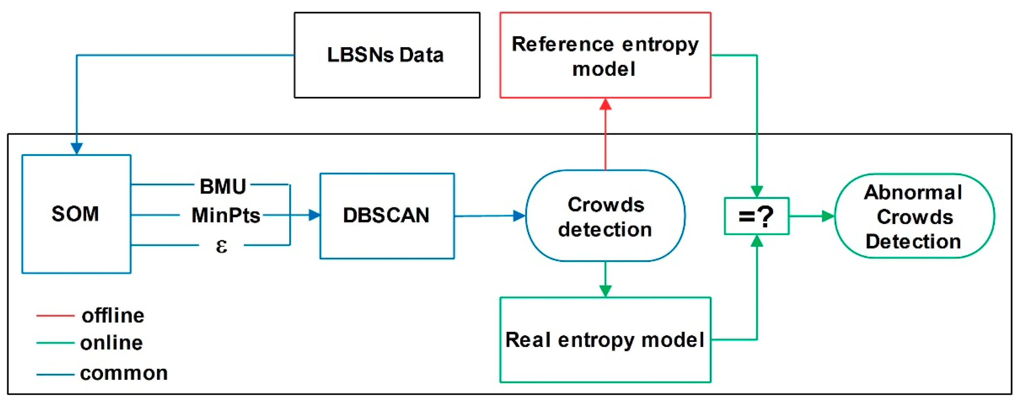
• Choose the parameters є and MinPts (Section 3.1).
• Establish DBSCAN (Section 3.1).
• Build the reference entropy model (Section 3.2).
• Build the real entropy model (Section 3.2).
• Compare the two models.

The studied city can be considered as a spatio-temporal model of an urban grouping composed of a set of circles, with each circle representing a grouping.

This model is instantiated t = 24 times if the time interval associates T = 60 min, and t = 48 times if T = 30 min. Each instance is associated with a set of symbols $\beta$ that define the state of the city under study. Thus, the behavior of the city is defined by a sequence S of i symbols $S=\left\{{\beta }_1,...,{\beta }_i\right\}$, with ${\beta }_i=\left\{G_1,...,G_k\right\}$ and k = 1,…, k is the number of crowds. Each group is defined by a circle of the center $C(latitud{e}_x,longitud{e}_y)$, the radius є and a MinPts density.

${\beta }_1=\left\{G_1,...,G_3\right\}=\left\{G_1(C_1,\epsilon ,MinPts),G_2(C_2,\epsilon ,MinPts),G_3(C_3,\epsilon ,MinPts)\right\}$ is the state of the city described by three groupings at the time interval $T_1$. From the entropy point of view, if the source $\mathrm{M}$ always sends the ${\beta }_1$ symbol, then its entropy according to Shannon [40] is nil, i.e., the uncertainty about what the source emits is minimal.

$\mathrm{H}\left(\mathrm{M}\right)$ is, therefore, a reference on the state of the city at this time interval. In this way, we can build a reference on the state of the city for the 24 h based on the Shannon entropy (the reference entropy model). To detect an abnormal grouping in the city, it is sufficient to determine the real entropy model and compare it with the reference model.

3.2. Real and Reference Entropy Models

For a discrete random variable M, with i symbols and each symbol ${\beta }_i$ having a probability of appearing ${\mathrm{P}}_i$, the entropy H of the source M is defined as follows:

$$H(\mathrm{M})=-\mathrm{E}\left[\log \mathrm{P}(\mathrm{M})\right]={\displaystyle \sum _{i=1}^i{\mathrm{P}}_i\log (\frac{1}{{\mathrm{P}}_i})}=-{\displaystyle \sum _{i=1}^i{\mathrm{P}}_i\log {\mathrm{P}}_i},$$

(6)

where E denotes the mathematical expectation, and log is the logarithm function. The symbols representing the possible achievements of the random variable M are $\left\{{\beta }_1,...,{\beta }_i\right\}$. To build the reference entropy model, look for the nil entropies of M at each interval:

$$H(\mathrm{M})=-{\displaystyle \sum _{i=1}^i({\mathrm{P}}_i=({\beta }_i))\log ({\mathrm{P}}_i=({\beta }_i))},$$

(7)

$${\mathrm{P}}_i=\frac{{\beta }_i}{{\displaystyle \sum _{j=1}^k{\beta }_j}},$$

(8)

$$\begin{array}{l}({\mathrm{P}}_i={\beta }_i)=\mathrm{P}(\left\{G_1,...,G_k\right\})\\ ({\mathrm{P}}_i={\beta }_i)=\mathrm{P}(\left\{G_1(C_1,\epsilon ,MinPts),...,G_k(C_k,\epsilon ,MinPts)\right\}),\end{array}$$

(9)

As є and MinPts are provided by DBSCAN and SOM to the already known time interval T, then Equation (9) is written as follows:

$$\begin{array}{l}({\mathrm{P}}_i={\beta }_i)=\mathrm{P}(\left\{C_1,...,C_k\right\})\\ ({\mathrm{P}}_i={\beta }_i)=\mathrm{P}(C_1),...,\cap \mathrm{P}(C_k)\\ ({\mathrm{P}}_i={\beta }_i)=\mathrm{P}((latitud{e}_1,longitud{e}_1)),...,\cap \mathrm{P}((latitud{e}_k,longitud{e}_k))\end{array}$$

(10)

where P_i is the probability of occurrence of the $\left\{C_1,...,C_k\right\}$ locations in a sequence of j measurements for each time interval T. That is to say, the number of times each symbol appears is β divided by j.

$$\begin{array}{l}\mathrm{P}({\beta }_i)=\frac{\mathrm{number} \mathrm{of} \mathrm{appearance} \mathrm{of} {\beta }_i=\left\{C_1,...,C_k\right\}}{j}\\ \mathrm{P}({\beta }_i)=\frac{\mathrm{P}(C_1),...,\cap \mathrm{P}(C_k)}{j}\end{array}$$

(11)

The reference model (for the normal day) is then constructed offline for a period of 28 days, i.e., four tests for each time interval T.

For the For the reference model, we keep the range of the minimum entropy of the source defined by the [min(entropy), max(entropy)].For example, for T = [00:00,00:30] and by applying SOM and DBSCAN, the possible realizations of the source are $\left\{{\beta }_1,{\beta }_2\right\}$ So, we calculate I = 6 measurements for the possible realizations of source M, which describe the state of the city at the time interval T, the results is shown in

Table 1. Example of the reference interval of entropy.

Measurements		1	2	3	4	5	6	H
First Monday	${\beta }_1$	✓	✓	✓	✓	✕	✕	0.276
	${\beta }_2$	✕	✕	✕	✕	✓	✓
Second Monday	${\beta }_1$	✓	✓	✓	✓	✓	✕	0.499
	${\beta }_2$	✕	✕	✕	✕	✕	✓
Third Monday	${\beta }_1$	✓	✓	✓	✓	✓	✕	0.499
	${\beta }_2$	✕	✕	✕	✕	✕	✓
Forth Monday	${\beta }_1$	✓	✓	✓	✕	✕	✕	0.300
	${\beta }_2$	✕	✕	✕	✓	✓	✓

.

The entropy of the source for the first normal Monday is therefore:$H_1(M)=-{\displaystyle \sum _{i=1}^{2}p({\beta }_i})+\log (p({\beta }_i))=-\left((\frac{4}{6}\times \log (\frac{4}{6})+(\frac{2}{6}\times \log (\frac{2}{6})\right)=0.276$. The reference interval of entropy for a Monday at the time interval $T_1$ is $E{T}_1$ = [0.276,0.499]. A day is said normal if and only if it is normal to all $T_i$.

3.3. Capturing Tweets

According to the literature, geo-localized tweets represent “1% of the total feed” [40]. "Tweet geo-localized" is associated with a geographic coordinate (latitude and longitude). The public streaming from which we gather the tweets is made available by Twitter API. However, Twitter’s data is not accessible to the general public. Officially, 1% of the tweet traffic is made available [40,41]. This sample of tweets in the form of streams is issued according to a user-defined criterion (geo-location or keywords).

Generally, there are three different ways to catch Twitter data: Firehose API, Twitter Search API, and the Twitter Streaming API. Through the Search API, users request tweets that match some sort of “search” criteria. The criteria can be keywords, usernames, locations, named places, etc. A good way to think of the Twitter Search API is by thinking how an individual user would do a search directly at Twitter. According to the documentation, Twitter Search API is limited by the number of requests per time, currently limited to 180 requests in 15 min. Unlike Twitter’s Search API where you are polling data from tweets that have already happened, Twitter’s Streaming API is a push of data as tweets happen in near real-time. The final way to access data is by having access to the full Twitter Firehose. The Twitter Firehose is in fact very similar to the Twitter’s Streaming API as it pushes data to end users in near real-time. However, the Twitter Firehose guarantees delivery of 100% of the tweets that match your criteria, but it is not free.

In this work, we use Twitter’s Streaming API due to the following reasons: the amount of data provided, Twitter’s Streaming API is certainly better than Twitter’s Search API, the nearly real-time data-set, the possibility of specifying the region of study (a shape formed by two geographic coordinates), and it is free.

4. Experiments

4.1. Data Sets

In this study, we classified the corpus of the gathered tweets into three datasets. The first one is for the special day; from 31 December 2017 at 15:00 to 1 January 2018 at 15:00 in NYC with 207,452 tweets and from 31 December 2017 at 15:00 to 1 January 2018 at 15:00 in Madrid with 67,152 tweets. The second one is for 28 normal days; the first four weeks of January, February, March and April 2017 in NYC and Madrid (to build the reference entropy model). The third dataset concerns the tweets collected between 15 August and 15 January 2019 and has 5,203,295 tweets, of which 270,060 are geolocated, while 5.1% are located in NYC and Madrid.

The first dataset “for the special day, from 15:00 of 31 December 2017 to 15:00 of 1 January 2018”, was selected to study the behaviour of the city during a special day and also to validate the effectiveness of our approach to the detection of an abnormal day. The second datasets were selected to build the reference entropy model. The last one was selected to determine whether the proposed approach is able to detect the abnormal days during this period based on the constructed reference model. Several works have followed the same procedure. In [21], the authors used the Streaming API, to obtained four datasets: one for the special day (from 15:00 of 31 December 2013 to 15:00 of 1 January 2014) and another for a normal day (from 15:00 of 24 February 2014 to 15:00 25 February 2014) in both cities (NYC and Madrid). In [23], the authors used a data set including both normal days and special days, due to festivities like Christmas or natural phenomena like the weekend when Storm Jonas hit the United States, which can be used to test the outlier detection because these dates are supposed to have an uncommon behaviour (higher densities in Christmas, lower during the Storm). The study in [40] relied on one full year of geolocated tweets, which were posted by users all over the world from 1 January until 31 December 2012. The database consists of 944 M records generated by a total of 13 M users.

4.2. Reference Area

Before applying the clustering stage and the real and reference entropy model, it is necessary to define a reference area. In NYC, we selected Times Square as the reference area, the most popular area in Manhattan, where people gather for New Year’s Eve. The studied area is defined by the central point P1(−73.985131, 40.758895) and a radius of 500 m. In Madrid, we selected Puerta del Sol as the reference area defined by the central point P2(40.416729, −3.703339) and a radius of 500 m.

The results are summarized in

Table 2. SOM and DBSCAN, first stage clustering results in a normal day in NYC.

Time (h)	ε	MinPts	Number of Clusters	Noise Points
15.00	30.12	3	1003	2654
16.00	23.41	2	732	2641
17.00	32.15	3	460	3546
18.00	26.21	3	422	4023
19.00	31.25	3	503	4895
20.00	35.10	4	360	5614
21.00	33.95	6	421	6210
22.00	38.25	5	556	5698
23.00	39.88	6	223	4512
00.00	42.50	5	197	4542
01.00	98.54	7	120	986
02.00	75.26	8	87	879
03.00	149.90	6	63	542
04.00	79.90	6	44	436
05.00	49.90	2	3	125
06.00	40.26	2	132	231
07.00	41.31	3	527	1895
08.00	33.25	3	301	1845
09.00	35.26	2	203	1954
10.00	37.21	3	489	2695
11.00	30.12	4	586	2828
12.00	35.11	3	991	3216
13.00	33.45	2	713	2963
14.00	33.21	3	633	3015

: Settlers (1) represent the time interval, (2) and (3) the values of the input parameters, (4) the number of clusters in NYC and (5) the noise points.

4.3. Results

At first glance, we notice that the obtained result in Table 2 shows that the number of detected clusters is clearly lower at night [00:00, 06:00]. The results, presented in Figure 3, show a higher number of clusters during the special day. It also shows that, the number of crowds decreases from 22:00 to 05:00, and then, increases again. Except for the interval [05:00, 09:00], the detected number of clusters is remarkably higher during the New Year’s Eve day than a normal day.

Therefore, we clearly see a contrast between both days. A comparison, between the number of crowds detected in the normal day (blue) and in the New Year’s Eve day, emphasizes the effectiveness of our system for crowd detection and distinguishes between the normal and the special days. The procedure for measuring/estimating parameters (є and MinPts) assumes a cautious process for clusters detection, without missing or disguising the small crowd.

An examination and analysis of the results of Table 2 and

Table 3. SOM and DBSCAN, first stage clustering results in the New Year’s Eve day in NYC.

Time (h)	ε	MinPts	Number of Clusters	Noise Points
15.00	10.22	3	703	7641
16.00	11.32	2	1193	6631
17.00	14.12	3	1181	6521
18.00	11.32	3	1198	6579
19.00	10.65	2	898	6984
20.00	9.55	3	989	7285
21.00	11.65	3	720	9875
22.00	10.11	3	948	6578
23.00	9.75	4	1302	5487
00.00	7.91	5	1214	4987
01.00	38.54	2	519	1245
02.00	45.26	2	401	1574
03.00	46.90	2	420	1578
04.00	59.90	5	196	987
05.00	57.90	5	87	995
06.00	40.26	5	68	898
07.00	41.31	3	72	2458
08.00	33.25	3	130	2657
09.00	35.26	2	412	4578
10.00	37.21	3	702	4884
11.00	30.12	3	1108	4369
12.00	35.11	3	703	5698
13.00	33.45	3	1609	5321
14.00	33.21	2	811	4578

show how the є and MinPts parameters affect the results of the clustering. It represents a dynamic system for the є and MinPts parameters selection. Values of these parameters are considered each hour and are obtained from the geolocated tweets.

Table 2 and Table 3 show how є and MinPts parameters selection using SOM (Section 3.1) affects the DBSCAN algorithm results. The SOM parameters selection process adopts a conservative approach, and preserves the topology of the data through the use of the neighborhood function, which allows detection of the clusters (even if they are small). Focusing on the number of clusters in the normal and special day of both Table 2 and Table 3, we note that the number of clusters in the New Year’s Eve day in NYC is always higher than in the normal day, except for a very few cases, which is evidence of something unusual happening in the city.

Figure 3 illustrates a comparison between the number of clusters obtained on the normal day and the New Year’s Eve day in NYC.

Table 4. SOM and DBSCAN, first stage clustering results in New Year’s Eve, 2018 in Madrid city.

Time (h)	ε	MinPts	Number of Clusters	Noise Points
15.00	41.52	5	415	442
16.00	40.70	5	514	362
17.00	49.21	4	421	512
18.00	51.65	5	512	532
19.00	49.25	4	320	566
20.00	48.65	4	125	541
21.00	44.65	5	125	545
22.00	42.15	5	210	566
23.00	39.88	3	145	495
00.00	49.50	2	99	488
01.00	54.34	2	52	458
02.00	65.26	2	44	365
03.00	75.91	5	14	145
04.00	74.84	7	8	102
05.00	59.69	2	7	44
06.00	54.56	2	55	46
07.00	53.11	2	220	456
08.00	53.65	2	321	514
09.00	45.26	2	455	395
10.00	47.21	3	551	546
11.00	49.52	3	326	321
12.00	41.58	3	281	301
13.00	39.92	3	332	402
14.00	40.59	3	336	306

show the number of clusters obtained in New Year’s Eve, 2018 in Madrid city and the dynamics of the є and MinPts parameters selection.

The number of clusters obtained on New Year’s Eve exceeds the values obtained on the normal day with exception of the time interval [06:00, 08:00]. The maximum value of the number of clusters for the special day is 1600 clusters and is reached at around 13:00. Celebrations of New Year’s Eve are clearly manifested by the evolution of the number of clusters in the interval [21:00, 23:00], unlike the behavior of the city on a normal day, when its residents go to sleep.

The ε values were calculated each hour, and are logically higher in the normal day compared to the special day when people began to come together to celebrate.

Figure 4 shows the discrepancy in the number of clusters during 24 h in Madrid city within 300 m of Puerta del Sol. This obviously confirms the dissimilarity behavior on a special and a normal day, so we can give a clear picture of the activity and the locations of the urban crowds in the city. Thus, it can be used (SOM and DBSCAN stage) to build with confidence the real and reference entropy models.

Subsequently, we focused first on the reference entropy model for each day, and then we compared it to the real entropy model, to detect anything unusual about the crowd behavior in the city.

Figure 5 illustrates a comparison of the number of clusters for 24 h in Madrid and NYC on New Year’s Eve of 2018. With the dominance of Facebook users in Spain, it is not possible to compare the crowd activity in both cities. However, the urban activity (rest times, working and commuting hours) was clearly detected by our approach, where it actually decreases in the time interval [00:01, 05:00].

To determine the entropy reference interval for every day of the week, we calculated the maximum and minimum entropy values for each time interval T during the first four weeks of January, February, March and April 2017, i.e., four measurements for each T of every day, and we kept the obtained average. For a normal Monday, the entropy values in T₁ = [00:00,01:00] are between [0.0344,0.3544].

Figure 6 shows a detailed description of the state of the city for the 7 days of the week for the time interval T = 60 min in New York City. The purple torque shows the evolution of the maximum and minimum reference value of the entropy for each day of the week. This reference is presented by the two lower and upper bounds that frame the possible values of the entropy of the possible realization of the source for a normal day. The blue curve represents the evolution of the entropy (6 measurements per time interval) of the source for a normal day.

Note that for the Friday entropy model shown in Figure 6 at time intervals [10:00,11:00] and [11:00,12:00], the value of the recorded entropy exceeds the upper limit of the reference. That is to say, for the six measurements of entropy, the source always returns the possible sequence of realization (presence of the possible sequence of realization for the six measurements). This can be explained either by an abnormal event at this interval that results in a stable state of the city, or by a false connection state, i.e., the tweet is not connected but is still considered online. In the following, we limit ourselves to four measurements for each time interval T to avoid false connections.

Looking at the effects that followed from the intense changes in entropy (blue curve) by the reference entropy model (purple torque), we found that, the entropy algorithm is properly applied to build the reference model. The entropy algorithm applies four measurements for each time interval T. However, this utility is very important for adapting the dynamics of crowds, which very quickly allows introspection of the creation of a new crowd in the short term. These results validate the proposed entropy approach that adapts the dynamics of the city, and we can look to the entropy process for anomaly detection with confidence.

The ε distance ranges from 21 to 150 m on the normal day and from 9 to 60 m on the New Year’s Eve day, as shown in Figure 7. Moreover, ε is usually lower on the special day than on the normal day. This means that a low value of ε designates more clusters closer to each other, which is consistent with a special day. In this study, we notice these differences, especially in the time interval [00:00, 06:00] where the differences between New Year’s Eve day and the normal day are remarkable. Now let’s focus on the variation of the MinPts parameter, where its least acute values vary from two to four tweets on the normal day in the time intervals [00:04, 20:00] and [00:06,23:00]. On a special day, these MinPts values are higher in the time interval [00:01, 00:02] and reflect low geo-tagged tweets and a low activity in the city.

Figure 8 shows the detection of special days in NYC. Each graph (a, b, c and d) shows the variation of the entropy value over 24 h, compared to the reference values. For the Hallows’ Eve on Wednesday, 31 October 2018 (a), we found three main things. First, the entropy value remains very close (on the lower boundary) to the reference for the time intervals [00:00, 03:00] and [05:00, 08:00]. However, if we compare it with the evolution of the entropy for a normal Wednesday in Figure 4, we can observe clearly that the entropy values are very far from the entropy values of the special day but in the reference interval. Second, the entropy value for the time intervals [10:00, 12:00] and [20:00,22:00] keeps the same pace as the reference (the lower boundary) and is also the same for New Year’s Eve, 2018 (d) for the time interval [00:00, 08:00]. This explains the similar behavior of tweets. Finally, the entropy values are within the range of the reference entropy model for the time intervals [13:00, 15:00] and [22:00, 23:00].

For the Memorial Day on Monday, 28 May 2018 (c), we noticed a entropy turmoil during the [16:00, 19:00] time interval, which explains an unstable state of the tweet’s behavior in this interval. We observed that the crowd’s behavior is customary at the [13:00,14:00] time interval.

5. Discussion

With the advent of smartphones, it is very interesting to propose a crowd detection system using the geolocated social network. The idea of density-based clustering for urban crowd detection has recently been applied to social network analysis [21,23,41,42,43]. Geo-tagged tweets allow one to detect real-world events from social network data. To analyze behavior of individual users in a geographical area under study, the preferred spatial clustering method is DBSCAN [21], a proposed density-based clustering method consisting of two main stages: A training stage and a detection stage. “For the first one it is necessary to mine LBSNs (one or more) in order to gather a representative set of geo-located users’ interactions (posts) and construct a geo-located dataset of the citizen’s activity (positions) all around the smart city for a whole day (24 h), the reference day. This dataset is analyzed by using a density-based clustering algorithm, with geographical proximity as distance, in order to detect dense groups of users located in the same geographical area at the same period of time”. However, using DBSCAN also involves problems. It can often be hard to choose the input parameters that should be used in high dimensional data due to the loss of contrast in the distances database. Furthermore, the LBSN data contains a large amount of information, and trying to find cluster patterns in several dimensions requires vast computing power. However, short computing time is always favorable. Last, the clusters can be arbitrary and complex, then finding these shapes can be very cumbersome. It therefore becomes difficult to use DBSCAN in high-dimensional data because of parameterization. In [23], the authors propose an improvement of [21], consisting of two main phases, to “compare the current activity in the social media stream on-the-fly with the reference cluster that is located in the same area on the same day of the week and at the same time interval. Therefore, the outlier’s detection is not performed equally for every cluster, but locally. This means that, instead of comparing the number of points of all the clusters in a wide area, a cluster is only compared with the nearest reference cluster (if there is one which is near enough to be considered as comparable)”. As such, DBSCAN parameterization in large data is difficult, prompting other studies to use the "Ordering points to identify the clustering structure (OPTICS)" algorithm, which is similar to DBSCAN, but addresses the problem of detecting meaningful clusters in data of varying density [23]. LSDBC, OPTICS, and HDBSCAN*, in “which the concept of border points was abandoned, and only core points are considered to be part of a cluster at any time, which is more consistent with the concepts of a density level set”, are examples of DBSCAN variants that focus on finding hierarchical clustering results [43], but still suffer from high dimensionality.

On the other hand, [44] introduced the concept of entropy and its practical interpretation. The proposed approach exploits the entropy behavior to minimize both drawbacks: the “anomalous data increase the entropy values, so no previous patterns are needed”, and the “entropy levels are continuously adapted as long as new geolocated data are extracted from social media”. The obtained results validated the effectiveness of the entropy-based social media location data and the methodology for crowd anomalies detection.

Furthermore, one of the strengths of the DBSCAN algorithm is that it can be paired with any data type, distance function (Euclidean, great-circle), and indexing technique adequate for the dataset to be analyzed. We therefore used SOM to mainly reduce the input space and enable parameter (є and MinPts) process selection, which then allows us to establish DBSCAN to handle the spatial and temporal properties of the Twitter data. With fertile ground to establish DBSCAN, this encourages us to propose urban crowd detection using the SOM, DBSCAN and LBSN data entropy methodology.

In this work, we use geolocated social data provided by the twitter API to automatically detect and identify an urban grouping. The crowd detection relies successively on two stages:

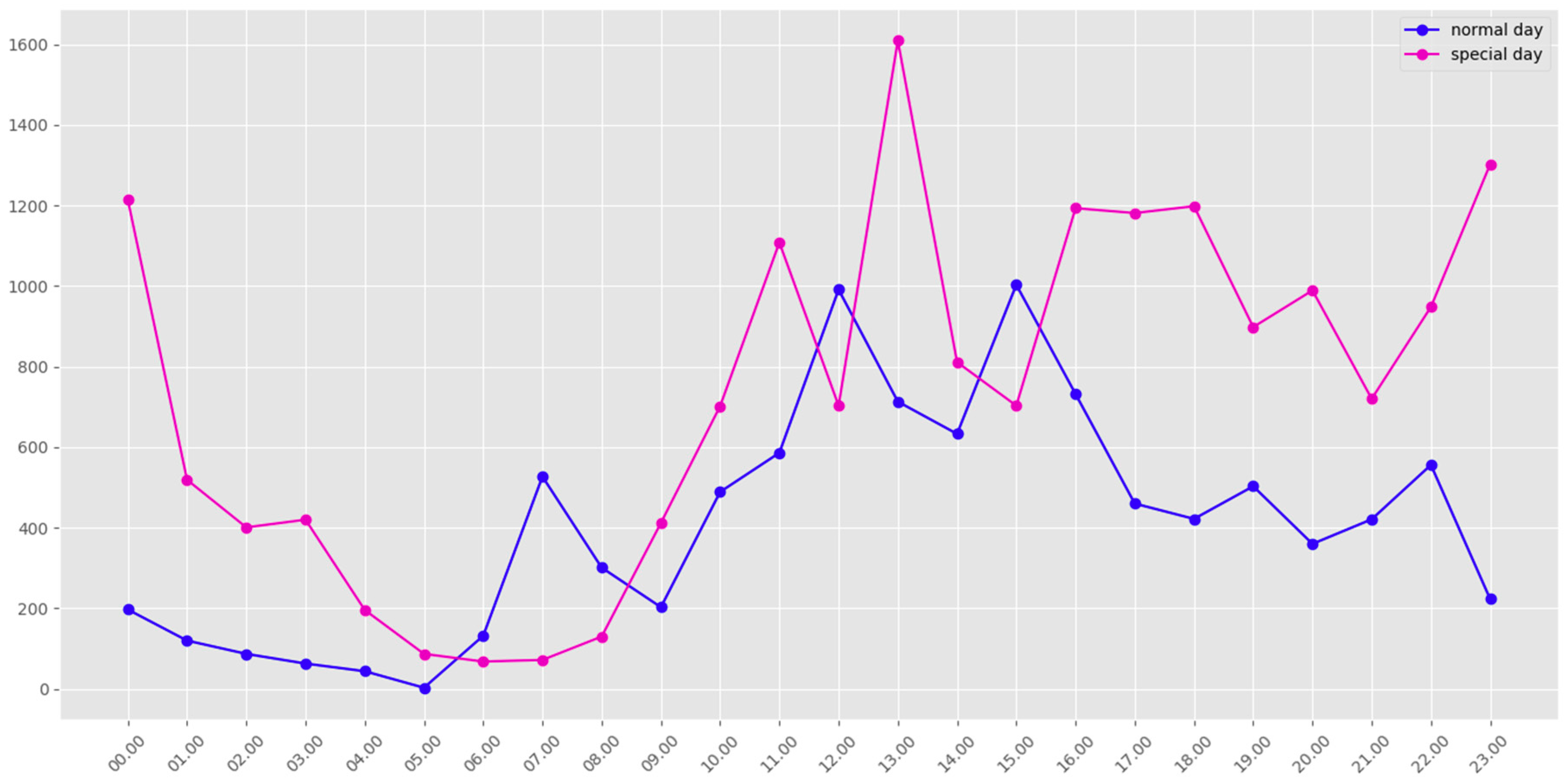
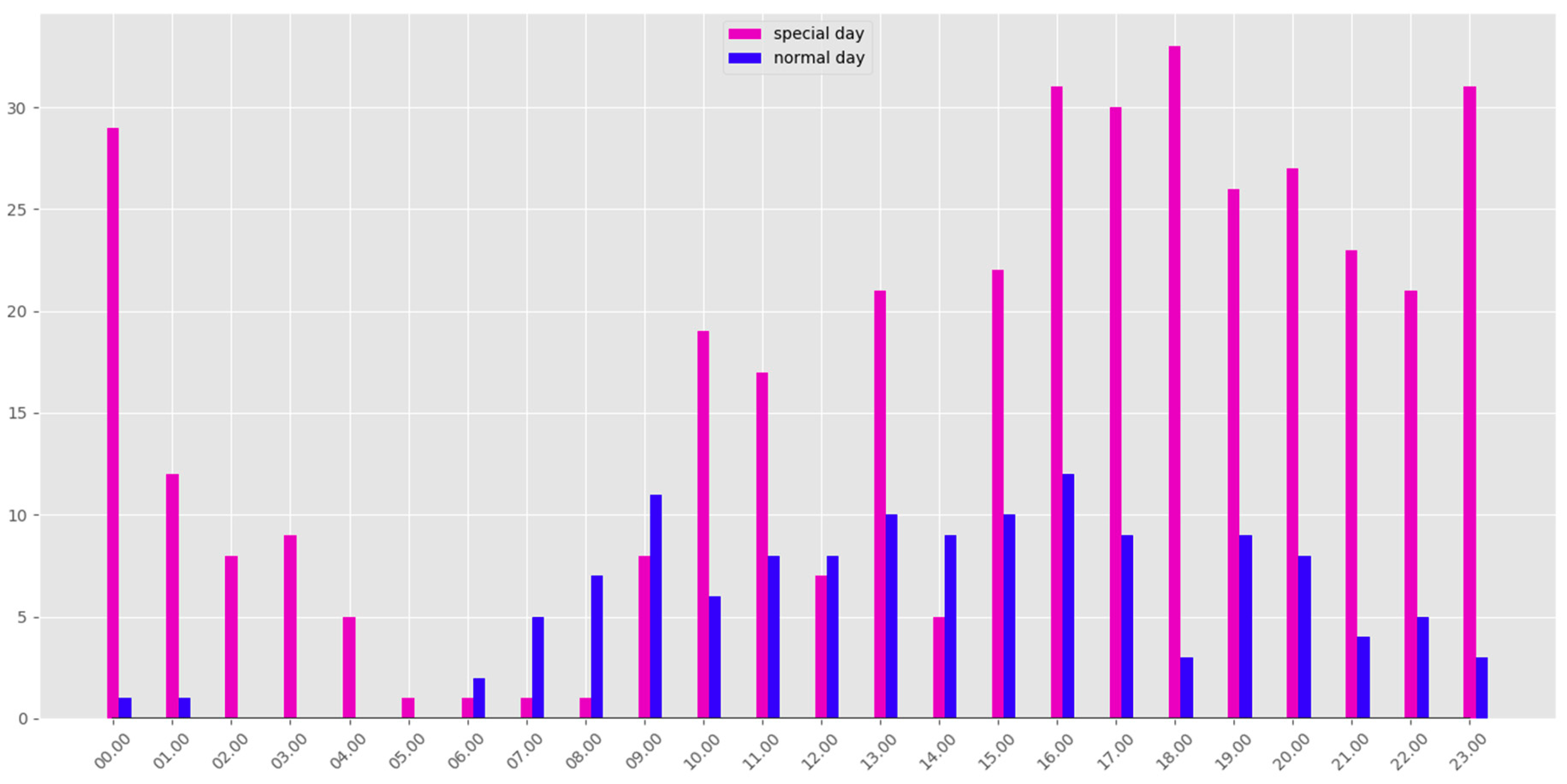
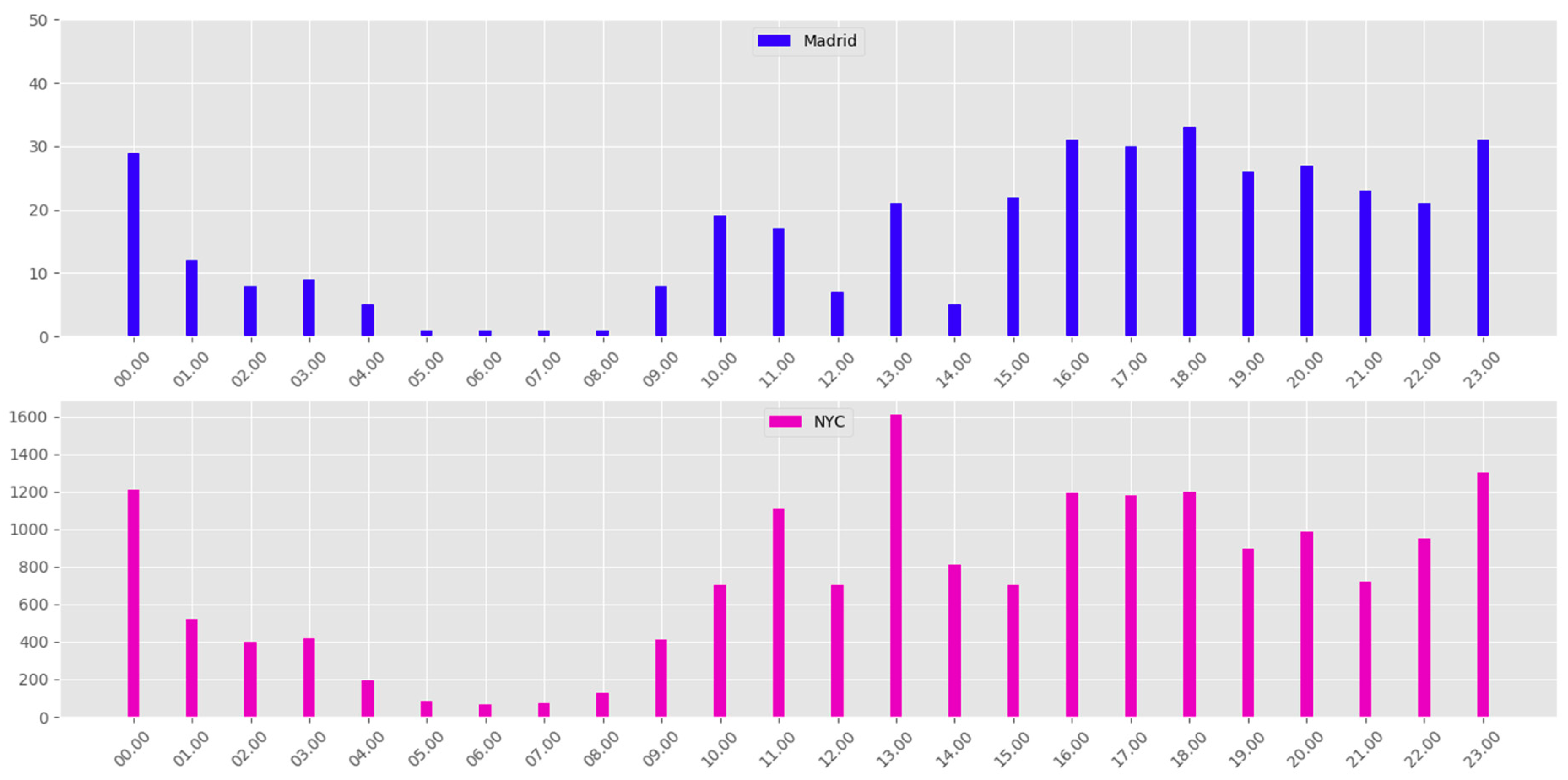
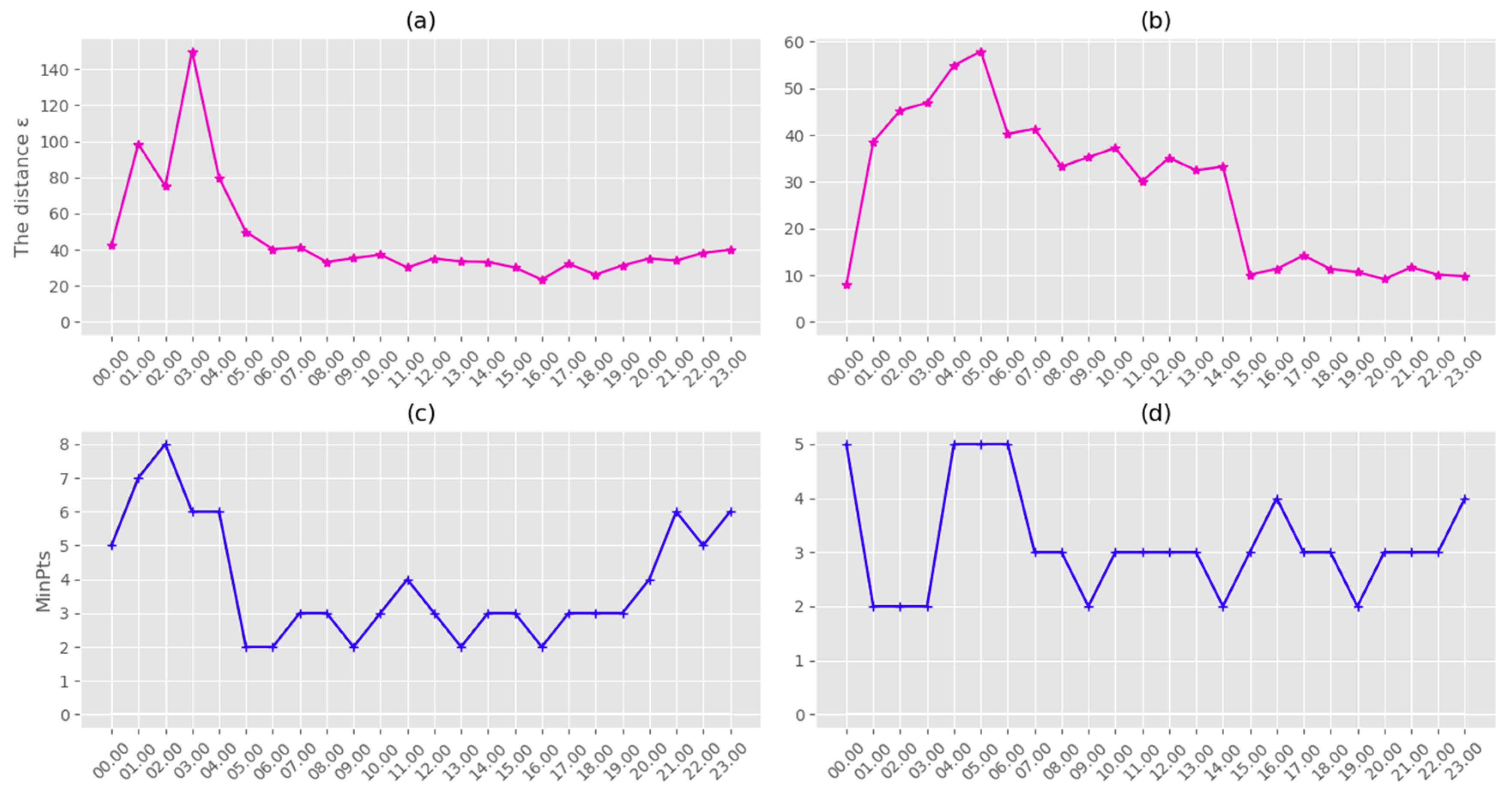
• The SOM (unsupervised clustering algorithm) and DBCSAN (density-based clustering algorithm) stage to identify and detect the crowds. This SOM and DBCSAN method for tweets clustering is well described in Section 3.1. Table 2, Table 3, Table 4 and Figure 4 summarize the obtained clustering results in NYC and Madrid city. The obtained results helped create a tool to support the abnormal events detection process, so this was a very important step. Figure 3, Figure 4 and Figure 5 show a detailed description of the state of the city on normal and special days in Madrid and NYC, illustrating the activity and the locations of the urban crowds. Figure 7 shows the dynamics of our system for estimating the parameters є and MinPts. All these results confirm the effectiveness of our method used in the first stage to detect and identify clusters dynamically, and imitating human nature movements. Therefore we have a robust methodology for identifying and detecting crowds that we can rely on.
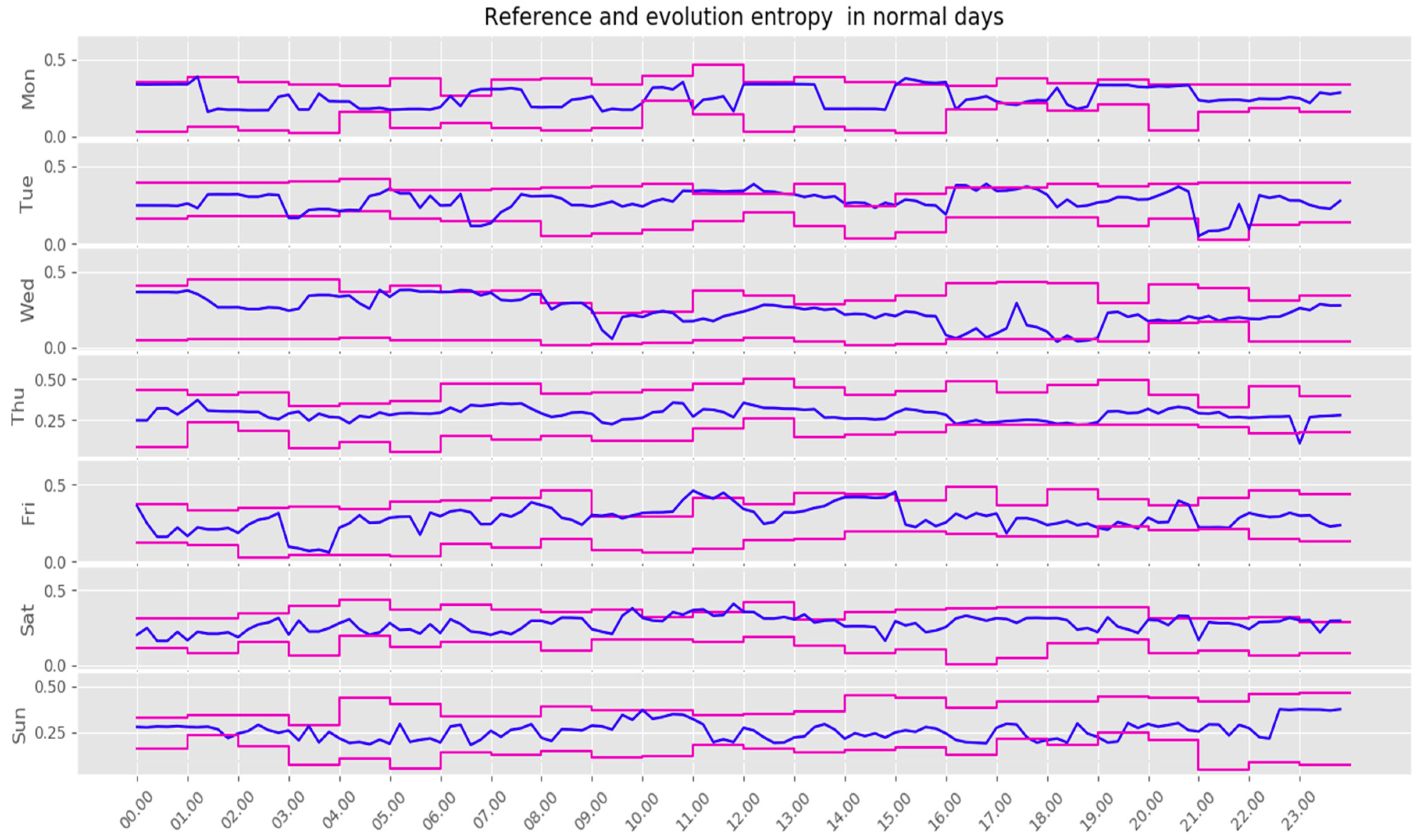
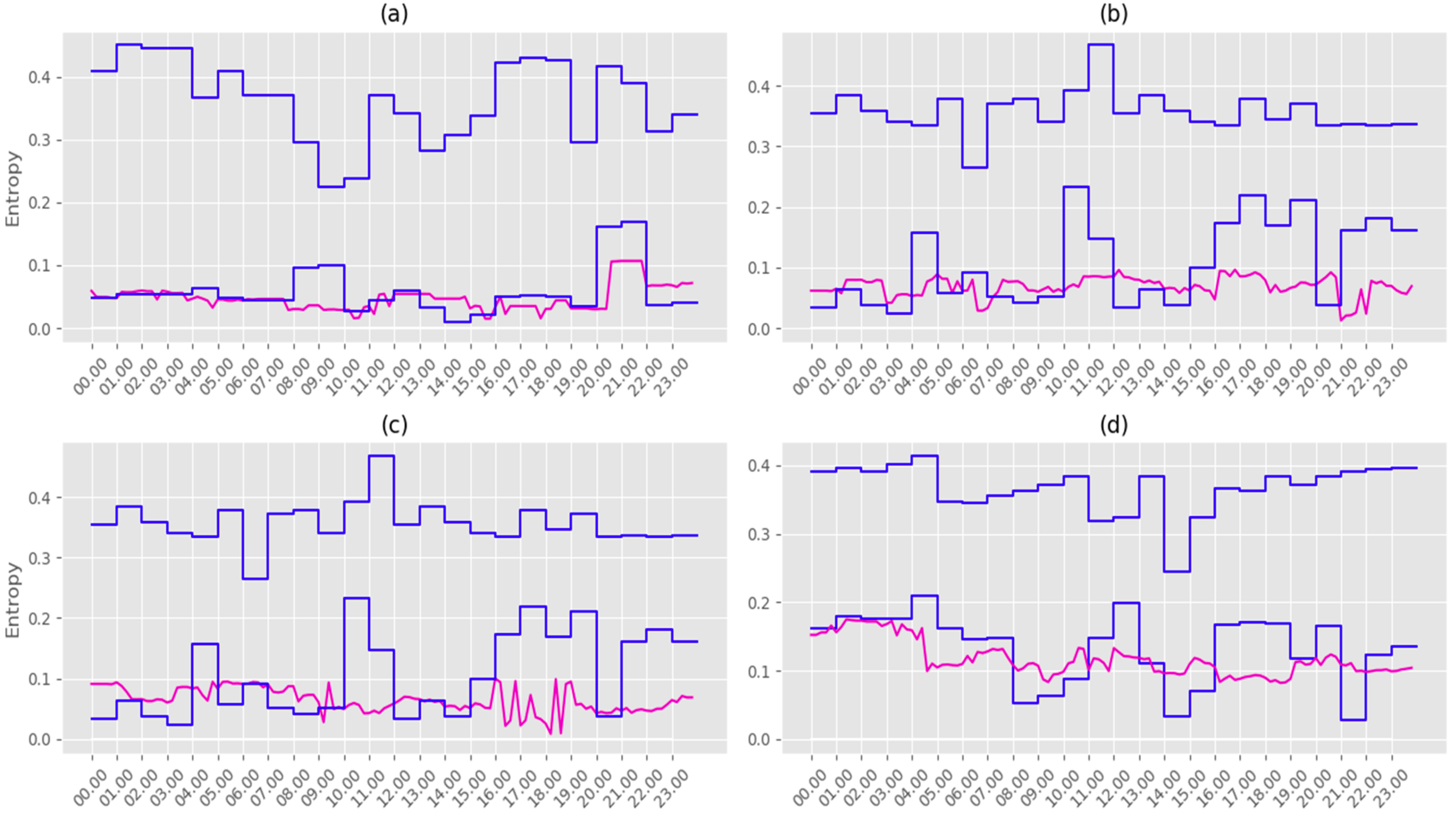
• The entropy model was applied to detect abnormal events in the crowds. The reference entropy model was then constructed offline. Figure 6 illustrates the evolution of the maximum and minimum reference value of the entropy for each day of the week. Figure 8 shows clearly the detection of special days in NYC, and proves the performances of our proposed model to determine whether the detected crowds fit into the daily pattern, or if they should be considered as evidence of something unusual happening in the city.
• The use of SOM in the first stage allows for:
  • Reducing the input space, which then allows us to establish DBSCAN. The DBSCAN algorithm is difficult to use in very large dimensions.
  • Using SOM to select є and MinPts parameters.
  • Using SOM and DBSCAN to detect the clusters of varied density with different shapes and sizes from the large amount of data, which contains noise and outliers.

The principal limit of using LBSN is the poor availability of geolocated tweets data. However, Twitter data is not accessible to the general public. Officially, 1% of the tweet traffic is made available [40,41]. Furthermore, it is a very interesting context for studying urban behavior.

6. Conclusions

Personal location and navigation have become a major field in a mobile society, especially with the huge Smartphone revolution coupled with the large number of social network users, where the daily produced data are now almost systematically linked to geographical coordinates. This technological revolution has unearthed a new type of service in the field of localization, known as LBSN services; these are applications available on mobile devices via the mobile network that use the geographic location of the mobile device. An LBSN does not only mean sharing our physical position with our friends, it also similarly reflects a natural urban structure. Precisely, in this context we propose a new system for urban crowd detection using SOMs, DBSCAN and entropy based on the LBSN of the most popular public social network, i.e., Twitter.

The proposed system in this paper consists of two stages. The first one is successively based on the unsupervised clustering algorithm SOM and the density-based clustering algorithm DBCSAN to identify and detect crowds. The use of SOM in the first stage has the following objectives: first, to provide a topological view of the partitioning of the data and second, to allow us to propose an appropriate procedure for selecting the necessary parameters for the DBSCAN algorithm in order to make the algorithm usable with big databases. Once the DBSCAN parameters are obtained they will not be applied to the entire data space but to the BMUs set as explained in Section 3.1. The SOM and DBSCAN step help identify and detect urban crowding. This will improve the robustness of our system to detect abnormal events in the crowds. The second stage, is to build a daily city-state reference based on the Shannon entropy (the reference entropy model). To detect an abnormal event, it is sufficient to determine the real entropy model and to compare it with the reference model (Section 3.1).

The concept of the abnormal event detection approach can be summarized as follows: identification and detection of clusters (SOM + DBSCAN), building the reference and the real entropy models, and finally comparing the two models. The obtained results prove the correctness and robustness of our method.

References

1. Flickr. Available online: http://www.flickr.com (accessed on 3 June 2018).
2. Foursquare. Available online: https://fr.foursquare.com (accessed on 3 June 2018).
3. Crampton, J.W.; Graham, M.; Poorthuis, A.; Shelton, T.; Stephens, M.; Wilson, M.W.; Zook, M. Beyond the Geotag: Situating ‘Big Data’ and Leveraging the Potential of the Geoweb. Cartogr. Geogr. Inf. Sci. 2013, 40, 130–139. [Google Scholar] [CrossRef]
4. Goodchild, M.F. Citizens as Sensors: The World of Volunteered Geography. GeoJournal 2007, 69, 211–221. [Google Scholar] [CrossRef]
5. Tang, K.P.; Lin, J.; Hong, J.I.; Siewiorek, D.P.; Sadeh, N. Rethinking Location Sharing: Exploring the Implications of Social-Driven vs. Purpose-Driven Location Sharing. In Proceedings of the 12th ACM International Conference on Ubiquitous Computing, UbiComp ’10, Copenhagen, Denmark, 26–29 September 2010; ACM: New York, NY, USA, 2010; pp. 85–94. [Google Scholar]
6. Stefanidis, A.; Crooks, A.; Radzikowski, J. Harvesting Ambient Geospatial Information from Social Media Feeds. GeoJournal 2013, 78, 319–338. [Google Scholar] [CrossRef]
7. Gordon, E.; e Silva, A.D.S. Urban Spaces. In Net Locality: Why location matters in a networked world; John Wiley & Sons, Ltd.: Hoboken, NJ, USA, 2011; pp. 85–104. [Google Scholar]
8. Couronné, T.; Raimond, A.-O.; Smoreda, Z. Looking at Spatiotemporal City Dynamics through Mobile Phone Lenses. In Proceedings of the 2011 International Conference on the Network of the Future, Paris, France, 28–30 November 2011; pp. 128–134. [Google Scholar]
9. Reades, J.; Calabrese, F.; Ratti, C. Eigenplaces: Analysing Cities Using the Space–Time Structure of the Mobile Phone Network. Environ. Plan. B Plan. Des. 2009, 36, 824–836. [Google Scholar] [CrossRef]
10. Ahas, R.; Aasa, A.; Yuan, Y.; Raubal, M.; Smoreda, Z.; Liu, Y.; Ziemlicki, C.; Tiru, M.; Zook, M. Everyday Space–Time Geographies: Using Mobile Phone-Based Sensor Data to Monitor Urban Activity in Harbin, Paris, and Tallinn. Int. J. Geogr. Inf. Sci. 2015, 29, 2017–2039. [Google Scholar] [CrossRef]
11. González, M.C.; Hidalgo, C.A.; Barabási, A.-L. Understanding Individual Human Mobility Patterns. Nature 2008, 453, 779–782. [Google Scholar] [CrossRef] [PubMed]
12. Wang, M.-H.; Schrock, S.D.; Vander Broek, N.; Mulinazzi, T. Estimating Dynamic Origin-Destination Data and Travel Demand Using Cell Phone Network Data. Int. J. ITS Res. 2013, 11, 76–86. [Google Scholar] [CrossRef]
13. Schneider, C.M.; Belik, V.; Couronné, T.; Smoreda, Z.; González, M.C. Unravelling daily human mobility motifs. J. R. Soc. Interface 2013, 10, 20130246. [Google Scholar] [CrossRef] [Green Version]
14. Tatem, A.J.; Qiu, Y.; Smith, D.L.; Sabot, O.; Ali, A.S.; Moonen, B. The Use of Mobile Phone Data for the Estimation of the Travel Patterns and Imported Plasmodium Falciparum Rates among Zanzibar Residents. Malar J. 2009, 8, 287. [Google Scholar] [CrossRef]
15. Lu, X.; Bengtsson, L.; Holme, P. Predictability of Population Displacement after the 2010 Haiti Earthquake. Proc. Natl. Acad. Sci. USA 2012, 109, 11576–11581. [Google Scholar] [CrossRef]
16. Wesolowski, A.; Buckee, C.O.; Bengtsson, L.; Wetter, E.; Lu, X.; Tatem, A.J. Commentary: Containing the Ebola Outbreak—The Potential and Challenge of Mobile Network Data. PLoS Curr. 2014, 6. [Google Scholar] [CrossRef]
17. Louail, T.; Lenormand, M.; Cantu Ros, O.G.; Picornell, M.; Herranz, R.; Frias-Martinez, E.; Ramasco, J.J.; Barthelemy, M. From Mobile Phone Data to the Spatial Structure of Cities. Sci. Rep. 2014, 4, 5276. [Google Scholar] [CrossRef] [PubMed]
18. Williams, N.E.; Thomas, T.A.; Dunbar, M.; Eagle, N.; Dobra, A. Measures of Human Mobility Using Mobile Phone Records Enhanced with GIS Data. PLoS ONE 2015, 10, e0133630. [Google Scholar] [CrossRef] [PubMed]
19. Noulas, A.; Scellato, S.; Mascolo, C.; Pontil, M. An Empirical Study of Geographic User Activity Patterns in Foursquare. In Proceedings of the Fifth International AAAI Conference on Weblogs and Social Media, San Francisco, CA, USA, 17–21 July 2011. [Google Scholar]
20. Kelley, M.J. The Emergent Urban Imaginaries of Geosocial Media. GeoJournal 2013, 78, 181–203. [Google Scholar] [CrossRef]
21. Ben Khalifa, M.; Díaz Redondo, R.P.; Vilas, A.F.; Rodríguez, S.S. Identifying Urban Crowds Using Geo-Located Social Media Data: A Twitter Experiment in New York City. J. Intell. Inf. Syst. 2017, 48, 287–308. [Google Scholar] [CrossRef]
22. Gao, H.; Liu, H. Data Analysis on Location-Based Social Networks. In Mobile Social Networking: An Innovative Approach; Chin, A., Zhang, D., Eds.; Computational Social Sciences; Springer New York: New York, NY, USA, 2014; pp. 165–194. [Google Scholar]
23. Domínguez, D.R.; Díaz Redondo, R.P.; Vilas, A.F.; Khalifa, M.B. Sensing the City with Instagram: Clustering Geolocated Data for Outlier Detection. Expert Syst. Appl. 2017, 78, 319–333. [Google Scholar] [CrossRef]
24. Pelechrinis, K.; Quercia, D. Urban informatics and the web. In Proceedings of the 24th International Conference on World Wide Web, Florence, Italy, 18–22 May 2015; p. 1547. [Google Scholar]
25. Silva, T.H.; Melo, P.O.S.V.D.; Almeida, J.M.; Loureiro, A.A.F. Large-Scale Study of City Dynamics and Urban Social Behavior Using Participatory Sensing. IEEE Wirel. Commun. 2014, 21, 42–51. [Google Scholar] [CrossRef]
26. De Nadai, M.; Staiano, J.; Larcher, R.; Sebe, N.; Quercia, D.; Lepri, B. The Death and Life of Great Italian Cities: A Mobile Phone Data Perspective. In Proceedings of the 25th International Conference on World Wide Web, WWW ’16, Montréal, QC, Canada, 11–15 April 2016; International World Wide Web Conferences Steering Committee: Republic and Canton of Geneva, Switzerland, 2016; pp. 413–423. [Google Scholar]
27. Roberts, H.V. Using Twitter Data in Urban Green Space Research: A Case Study and Critical Evaluation. Appl. Geogr. 2017, 81, 13–20. [Google Scholar] [CrossRef]
28. Comito, C.; Falcone, D.; Talia, D. Mining Human Mobility Patterns from Social Geo-Tagged Data. Pervasive Mobile Comput. 2016, 33, 91–107. [Google Scholar] [CrossRef]
29. Kanno, M.; Ehara, Y.; Hirota, M.; Yokoyama, S.; Ishikawa, H. Visualizing High-Risk Paths Using Geo-Tagged Social Data for Disaster Mitigation. In Proceedings of the 9th ACM SIGSPATIAL Workshop on Location-based Social Networks, LBSN16, Burlingame, CA, USA, 31 October–3 November 2016; ACM: New York, NY, USA, 2016; pp. 4:1–4:8. [Google Scholar]
30. Kim, K.-S.; Kojima, I.; Ogawa, H. Discovery of Local Topics by Using Latent Spatio-Temporal Relationships in Geo-Social Media. Int. J. Geogr. Inf. Sci. 2016, 30, 1899–1922. [Google Scholar] [CrossRef]
31. Yang, J.; Hauff, C.; Houben, G.-J.; Bolivar, C.T. Diversity in Urban Social Media Analytics. In Web Engineering; Bozzon, A., Cudre-Maroux, P., Pautasso, C., Eds.; Lecture Notes in Computer Science; Springer International Publishing: Lugano, Switzerland, 2016; pp. 335–353. [Google Scholar]
32. Bordogna, G.; Frigerio, L.; Cuzzocrea, A.; Psaila, G. Clustering Geo-Tagged Tweets for Advanced Big Data Analytics. In Proceedings of the 2016 IEEE International Congress on Big Data (BigData Congress), San Francisco, CA, USA, 27 June–2 July 2016; pp. 42–51. [Google Scholar]
33. Manca, M.; Boratto, L.; Morell Roman, V.; Martori i Gallissà, O.; Kaltenbrunner, A. Using Social Media to Characterize Urban Mobility Patterns: State-of-the-Art Survey and Case-Study. Online Soc. Netw. Media 2017, 1, 56–69. [Google Scholar] [CrossRef]
34. Gao, S.; Liu, Y.; Wang, Y.; Ma, X. Discovering Spatial Interaction Communities from Mobile Phone Data. Trans. GIS 2013, 17, 463–481. [Google Scholar] [CrossRef] [Green Version]
35. Ahas, R. Using Mobile Positioning Data for Mapping Space-Time Behavior and Developing LBS: Experiences from Estonia; Carto Talk: Tartu, Estonia, 2008. [Google Scholar]
36. Senaratne, H.; Mobasheri, A.; Ali, A.L.; Capineri, C.; Haklay, M. A Review of Volunteered Geographic Information Quality Assessment Methods. Int. J. Geogr. Inf. Sci. 2017, 31, 139–167. [Google Scholar] [CrossRef]
37. Kohonen, T. Self-Organizing Maps, 3rd ed.; Springer Series in Information Sciences; Springer: Berlin/Heidelberg, Germany, 2001. [Google Scholar]
38. Sakkari, M.; Ejbali, R.; Zaied, M. Deep SOMs for Automated Feature Extraction and Classification from Big Data Streaming. In Proceedings of the Ninth International Conference on Machine Vision (ICMV 2016), Nice, France, 8–20 November 2016; International Society for Optics and Photonics: Bellingham, WA, USA, 2017; Volume 10341, p. 103412. [Google Scholar]
39. Ester, M.; Kriegel, H.-P.; Sander, J.; Xu, X. A Density-Based Algorithm for Discovering Clusters a Density-Based Algorithm for Discovering Clusters in Large Spatial Databases with Noise. In Proceedings of the Second International Conference on Knowledge Discovery and Data Mining, KDD’96, Portland, OR, USA, 2–4 August 1996; AAAI Press: Menlo Park, CA, USA, 1996; pp. 226–231. [Google Scholar]
40. Hawelka, B.; Sitko, I.; Beinat, E.; Sobolevsky, S.; Kazakopoulos, P.; Ratti, C. Geo-located Twitter as proxy for global mobility patterns. Cartogr. Geogr. Inf. Sci. 2014, 41, 260–271. [Google Scholar] [CrossRef] [PubMed] [Green Version]
41. Morstatter, F.; Pfeffer, J.; Liu, H.; Carley, K.M. Is the Sample Good Enough? Comparing Data from Twitter’s Streaming API with Twitter’s Firehose. In Proceedings of the 7th International Conference on Weblogs and Social Media, ICWSM 2013, Cambridge, MA, USA, 8–11 July 2013; AAAI Press: Menlo Park, CA, USA, 2013; pp. 400–408. [Google Scholar]
42. Huang, Y.; Li, Y.; Shan, J. Spatial-Temporal Event Detection from Geo-Tagged Tweets. ISPRS Int. J. Geo-Inf. 2018, 7, 150. [Google Scholar] [CrossRef]
43. Schubert, E.; Sander, J.; Ester, M.; Kriegel, H.P.; Xu, X. DBSCAN Revisited, Revisited: Why and How You Should (Still) Use DBSCAN. ACM Trans. Database Syst. 2017, 42, 19:1–19:21. [Google Scholar] [CrossRef]
44. Garcia-Rubio, C.; Díaz Redondo, R.P.; Campo, C.; Fernández Vilas, A. Using Entropy of Social Media Location Data for the Detection of Crowd Dynamics Anomalies. Electronics 2018, 7, 380. [Google Scholar] [CrossRef]
Figure 1. Human mobility based on location-based social networks (LBSNs).
Electronics 08 00692 g001
Figure 2. Urban crowd detection.
Electronics 08 00692 g002
Figure 3. Clustering results in New York City on a normal day and New Year’s Eve day.
Electronics 08 00692 g003
Figure 4. Number of clusters from Puerta del Sol on normal and special days.
Electronics 08 00692 g004
Figure 5. NYC and Madrid city clustering results on a special day.
Electronics 08 00692 g005
Figure 6. Reference interval of entropy; the minimum and maximum entropy value for each interval (purple) and real entropy evolution (blue) for the 7 days of the week for the time interval T = 60 min in New York City.
Electronics 08 00692 g006
Figure 7. Fluctuation of the distance ε on a normal day (a) and a special day (b). The MinPts parameter value in the New Year’s Eve (c) and on a normal day (d).
Electronics 08 00692 g007
Figure 8. Abnormal day detection in NYC. (a) Hallows’ Eve on Wednesday, 31 October 2018. (b) Columbus Day on Monday, October 8, 2018. (c) Memorial Day on Monday, 28 May 2018. (d) New Year’s Eve, 2018.
Electronics 08 00692 g008