Control of Internal Dynamics of Grid-Connected Modular Multilevel Converter Using an Integral Backstepping Controller

Abstract

The modular multilevel converter (MMC) has significant applications in power systems due to its promising features, such as modularity, reliability, scalability, and low harmonic distortion. One of the challenges in the operation of MMC is to regulate the circulating current in its phase leg and sub module (SM) capacitor voltage. This paper presents the control of internal dynamics, i.e., circulating current and submodule capacitor voltage, of the MMC using an integral backstepping algorithm. The design of the controller is based on Lyapunov stability function. The backstepping control ensures the convergence of the error signal to zero. Additionally, the integral action in the control law increases the robustness and reliability of the system against the external disturbances and model uncertainties. Moreover, the integral term in the controller eliminates the residual steady-state error. The Lyapunov function-based design of the backstepping controller guarantees the convergence of circulating current as well as submodule capacitor voltage for any possible initial condition. Moreover, the performance of the proposed integral backstepping controller is compared with the proportional resonant (PR) controller. The proposed backstepping control scheme for three-phase MMC has been implemented in MATLAB/Simulink.

1. Introduction

The modular multilevel converter (MMC) has gained popularity due to it is in a wide range of applications, e.g., renewable energy integration with the grid, high voltage direct current (HVDC), and drive application. The domain of MMC is broadened due to its modular structure, use of low rating devices, low harmonic distortion, high efficiency, and energy storage system [1,2,3,4,5,6]. The structure of a three-phase grid-connected MMC is depicted in Figure 1.

However, the control of MMC is a challenging task due to many output variables and fewer input variables. The control of MMC is categorized into two types, i.e., output current control and internal dynamics control. The control of output current is an easy task as compared to internal control of MMC. In case of output current control, a variable is available for manipulation. With the control of output current, the power flow to the grid is controlled. However, the internal dynamics includes three state variables, i.e., circulating current, upper arm capacitor voltage, and lower arm capacitor voltage. These state variables make control of MMC more complicated. The main challenges in internal control are to minimize the magnitude of the second harmonic in the circulating current, balancing the capacitor voltage and internal energy of MMC. Although the circulating current has a second order negative sequence harmonic content, it has no impact on the grid-side AC current. However, if it is not controlled to a desired value, it will cause high power losses due to its high root mean square (RMS) value [7]. A specific arm inductor can be used to minimize the amplitude of circulating current but active control strategy is also needed to vanquish all unnecessary components. Researchers have proposed many control strategies for output current control and suppression of the second harmonic in the circulating current. In [8], the proportional resonant controller was proposed for the MMC. The controller is tuned at the fundamental frequency for the output current while for the circulating current, it is tuned at the frequency of the second harmonic. A proportional integral (PI) controller was proposed in [9]. The circulating current control is carried out in $dq-axis$ with double frequency rotating reference frame. Although these controllers have a simplified structure, the nonlinearity and coupling between the state variable of the MMC urges the development of new and more effective control structures. In [10], the researcher proposed a cascaded control structure along with phase shifted pulse width modulated (PS-PWM) scheme for controlling the internal and output parameters of the MMC. The proposed method lags when it comes to the effective suppression of the circulating current. Different feedback control schemes in the $dq$ frame are also proposed for suppression of circulating current [11,12,13].

In [14], multiple resonant controllers were developed for harmonic mitigation during load perturbation. The plug-in repetitive controller was also proposed to vanquish the harmonic contents in the circulating current [15,16,17]. All these control strategies are based on a cascaded control structure. The design and tuning of these control structures may be a difficult task while considering the performance and stability of the system. In addition to these control strategies, various nonlinear control methods are also developed to cope with the control problems in MMC. The model-based input-output linearization method [18], direct and indirect model-based predictive control [19,20,21,22], feedback linearization control [23,24], and langrange multiplier-based optimized control [25] are used for the control of the dynamics of the MMC. The computational burden of the model predictive control limits the real-time implementation of the control scheme. However, the rest of the control schemes need a fully developed mathematical model to effectively implement the control strategies.

In this paper, we have proposed a novel backstepping algorithm for the control of internal dynamics, i.e., circulating current and submodule capacitor voltage, and energy sum and energy difference of the MMC. The proposed control algorithm is designed based on the Lyapunov stability function. The Lyapunov based design of the proposed controller guarantees the convergence of error to zero. That regulates the circulating current and submodule capacitor voltage. The integral backstepping algorithm is developed for the control of the dynamics of the MMC. The integral action of the control algorithm will effectively eliminate the steady-state error produced due to the inaccuracy in the modeling of the system. The designed controller has robust behavior to the parameter variations, model uncertainties, and external perturbation in the system. The algorithm uses a Lyapunov function to converge the dynamics of the system. The performance of the controller in the results reflects our claim. Furthermore, the results of the proposed controller are compared with a proportional resonant controller for justification.

The structure of the rest of the paper is organized as follows: In Section 2, the modeling of the MMC is presented. The control design of a backstepping algorithm for our problem is formulated in Section 3. Section 4 is focused on results and discussion of the implemented control algorithm, and finally, the paper is concluded in Section 5.

2. Modeling of the MMC

The equivalent single-phase circuit of MMC is depicted in Figure 2 $R$ and $L$ represent the arm resistance and inductance respectively. $e_{u,j}$ is the arm generated voltages by sub module (SMs). The subscript ‘$u$’ and $l$ denote the upper and lower arm, respectively, while $j$ is used for phases $\left(j=a,b,c\right)$. $I_d$ and $V_d$ denote DC current and DC bus voltage. $v_j$ is used to represent the AC bus voltage.

The differential current of the MMC is defined as [26]:

$$i_{u,j}=i_{c,j}+\frac{i_{o,j}}{2}$$

(1)

$$i_{l,j}=i_{c,j}-\frac{i_{o,j}}{2}$$

(2)

$$i_{o,j}=i_{u,j}-i_{l,j}$$

(3)

$$i_{c,j}=\frac{1}{2}\left(i_{u,j}+i_{l,j}\right)$$

(4)

By applying Kirchhoff’s voltage law on the circuit Figure 2, we get the following voltage equations:

$$-\frac{1}{2}{V}_d+e_{u,j}+i_{u,j}R+L\frac{d{i}_{u,j}}{dt}+v_j=0$$

(5)

$$-\frac{1}{2}{V}_d+e_{l,j}+i_{l,j}R+L\frac{d{i}_{l,j}}{dt}-v_j=0$$

(6)

Adding and subtracting Equations (5) and (6) along with substitution of Equations (3) and (4) will result in the following set of equations:

$$\frac{L}{2}\frac{d{i}_{o,j}}{dt}=\underset{v_{s,j}}{\underbrace{\left(\frac{-e_{u,j}+e_{l,j}}{2}\right)}}-\frac{R}{2}{i}_{o,j}-v_j$$

(7)

$$L\frac{d{i}_{c,j}}{dt}=-\underset{v_{c,j}}{\underbrace{\left(\frac{e_{u,j}+e_{l,j}}{2}\right)}}-R{i}_{c,j}+\frac{V_d}{2}$$

(8)

Equations (7) and (8) characterize the dynamics of the MMC. $v_{s,j}$ is the output voltage of the converter respective phase “$j=a,b,c$” and $v_{c,j}$ is internal voltage. By analyzing Equation (7), it is concluded that $v_j$ is the AC bus voltage, hence, only $v_{s,j}$ can be manipulated to control the output current $i_{o,j}$. Similarly, Equation (8) is used to control the circulating current dynamics of the MMC. Likewise, in Equation (8) $i_{c,j}$ can be controlled by the manipulation of internal voltage $v_{c,j}$. Moreover, the internal dynamics of the SM capacitor is represented in term of arm voltages and arm currents as:

$$\frac{C}{N}\frac{d{v}_{cu,j}^{\Sigma }}{dt}=n_{u,j}^i{i}_{u,j}$$

(9)

$$\frac{C}{N}\frac{d{v}_{cl,j}^{\Sigma }}{dt}=n_{l,j}^i{i}_{l,j}$$

(10)

$C$ is the capacitance of the SM capacitor, $N$ represents the number of SM in arms while $v_{cu,j}^{\Sigma }$ and $v_{cl,j}^{\Sigma }$ are the sum capacitor voltage of the upper arm and lower arm, respectively. $n_{u,j}^i$ and $n_{l,j}^i$ represents insertion indices of the upper and lower arms, respectively. $(n_{u,j}^i$, $n_{u,j}^i)=1$ means that the capacitor is inserted while $(n_{u,j}^i$, $n_{u,j}^i)=0$ means that the capacitor is bypassed in respective arms. Equations (8), (9), and (10) in combination represents the internal dynamic of the MMC. Equations (1) and (2) are substituted into Equations (9) and (10) to represents Equations (9) and (10) in terms of output current, circulating current, and insertion indices ($n_u$, $n_l$).

$$\frac{1}{N}\frac{Cd{v}_{cu,j}^{\Sigma }}{dt}=n_u\left(i_{c,j}+\frac{i_{o,j}}{2}\right)$$

(11)

$$\frac{1}{N}\frac{Cd{v}_{cl,j}^{\Sigma }}{dt}=n_l\left(i_{c,j}-\frac{i_{o,j}}{2}\right)$$

(12)

While in the variables $n_u=\frac{v_c^{*}-v_s^{*}}{v_{cu}^{\Sigma }}$ and $n_l=\frac{v_c^{*}+v_s^{*}}{v_{cl}^{\Sigma }},$ $v_c^{*}$ and $v_s^{*}$ are the controlled inputs to the plant. The internal dynamics of the MMC is controlled through the convergence of $i_{c,j}$ to a DC component $\frac{P}{M{V}_d}$. $P$ is an active power, $M$ represents the number of phases. In internal dynamics control, $n_u$ and $n_l$ are available for manipulation. As well, $v_{cu}^{\Sigma }$ and $v_{cl}^{\Sigma }$ are forced to converge to $V_d$ for controlling the internal dynamics of MMC.

Equations (8), (11), and (12) represents the internal dynamics of MMC. With the state variables $i_{c,j}$, $v_{cu}^{\Sigma }$, and $v_{cl}^{\Sigma }$, the mathematical model of the MMC is represented in state space form as:

$$\frac{d}{dt}\left[\begin{array}{c}{i}_{c,j}\\ v_{cu}^{\Sigma }\\ v_{cl}^{\Sigma }\end{array}\right]=\left[\begin{array}{ccc}-\frac{R}{L}& -\frac{n_u}{2L}& -\frac{n_l}{2L}\\ \frac{N{n}_u}{C}& 0& 0\\ \frac{N{n}_l}{C}& 0& 0\end{array}\right]\left[\begin{array}{c}{i}_{c,j}\\ v_{cu}^{\Sigma }\\ v_{cl}^{\Sigma }\end{array}\right]+\frac{1}{2}\left[\begin{array}{c}\frac{V_d}{2}\\ \frac{N{n}_u{i}_{o,j}}{C}\\ -\frac{N{n}_l{i}_{o,j}}{C}\end{array}\right]$$

(13)

This model is computationally efficient for the internal dynamics of the MMC [27]. The output current of the MMC, insertion indices, and DC voltage is applied as input to the model. The model shows the inter relation of the output current, circulating current, insertion indices, DC bus voltage, and capacitor sum voltages of lower and upper arms. In this model the state of the MMC is described in terms of capacitor sum voltages. The states are being continuously updated on the insertion indices and arm current. The block representation of the MMC model is depicted in Figure 3. This representation makes the model simple to implement it in block-oriented form in MATLAB/Simulink, PSIM, PLECS, PSCAD, and other simulation software.

3. Control Design for Internal Dynamics

3.1. Integral Backsteeping Design Overview

The design of recursive Lyapunov-based backstepping algorithm is based on considering some of the state variables as a “virtual control” and designing a control law for them. The Lyapunov function is considered for the whole system while designing the algorithm. Hence, the controller achieves stabilization and acquires the ability to track due to the recursive computation in the algorithm. Due to these properties, the backstepping controller has robust behavior to the parameter variations, model uncertainties, and external perturbation in the system. To develop a clear idea, consider a non-linear system as follows [28,29]:

$$\{\begin{array}{c}{\dot{x}}_1=x_2\\ {\dot{x}}_2=f\left(x\right)+g\left(x\right)u\end{array}$$

(14)

where $x\in R^n$ is system state vector, $f\left(x\right)$ and $g\left(x\right)$ are a nonlinear function of the system state vector $\left(x\right)$ and input vector $\left(u\right)$. To converge the dynamics of system to the desired value. The error is defined as $e_1=x_1-x_{1d}$ where $x_{1d}$ is the desired value. Our objective is to converge the error to zero, i.e., $\left(e_1,{\dot{e}}_1\right)\to 0$. The control algorithm for a system is designed in two steps.

Step 1

By taking the derivative of error and replacing the value of ${\dot{x}}_1$

$${\dot{e}}_1={\dot{x}}_1-{\dot{x}}_{1d}=x_2-{\dot{x}}_{1d}$$

(15)

By choosing the Lyapunov function candidate to converge the error to zero, i.e., $e_1\to 0$

$$V_1=\frac{1}{2}{e}_1^2$$

(16)

By taking the derivative of the Lyapunov function Equation (16) and replace the value of ${\dot{e}}_1$ with Equation (15)

$${\dot{V}}_1=e_1{\dot{e}}_1=e_1\left(x_2-{\dot{x}}_{1d}\right)$$

(17)

${\dot{V}}_1<0$ ensures the stability of the system, hence, the derivative of error $\left({\dot{e}}_1\right)$ is equalize to $-c_1{e}_1$

$$x_2-{\dot{x}}_{1d}=-c_1{e}_1,\hspace{1em}{c}_1>0$$

(18)

Then

$${\dot{V}}_1=-c_1{e}_1^2$$

(19)

Equation (19) guarantees the stability condition.

Step 2

To attain $x_2-{\dot{x}}_{1d}=-c_1{e}_1$, that is $x_2={\dot{x}}_{1d}-c_1{e}_1$, a virtual control variable is chosen as:

$$x_{2d}={\dot{x}}_{1d}-c_1{e}_1$$

(20)

To attain $x_2\to x_{2d}$, a new error is introduced.

$$e_2=x_2-x_{2d}$$

(21)

Then take the derivative of the error and replace the value of ${\dot{x}}_2$ with Equation (14).

$${\dot{e}}_2={\dot{x}}_2-{\dot{x}}_{2d}=f\left(x\right)+g\left(x\right)u-{\dot{x}}_{2d}$$

(22)

To attain $e_2\to 0$ and $e_1\to 0$, a Lyapunov function is designed as:

$$V_2=V_1+\frac{1}{2}{e}_2^2=\frac{1}{2}\left(e_1^2+e_2^2\right)$$

(23)

Take the derivative and replace the value of ${\dot{e}}_1$ with Equation (15).

$${\dot{V}}_2=e_1\left(x_2-{\dot{x}}_{1d}\right)+e_2{\dot{e}}_2$$

(24)

Similarly, replacing the value of $x_2$ and ${\dot{e}}_2$ by Equations (21) and (22) we get

$$-c_1{e}_1^2+e_1{e}_2+e_2\left(f\left(x\right)+g\left(x\right)u-{\dot{x}}_{2d}\right)$$

(25)

To attain ${\dot{V}}_2<0$, we simplify Equation (25) and equate it to $-c_2{e}_2$

$$e_1+f\left(x\right)+g\left(x\right)u-{\dot{x}}_{2d}=-c_2{e}_2,\hspace{1em}{c}_2>0$$

(26)

Then

$${\dot{V}}_2=-c_1{e}_1^2-c_2{e}_2^2$$

(27)

From Equation (26), consider ${\dot{x}}_{2d}={\ddot{x}}_{1d}-c_1{\dot{e}}_1$, and we will obtain control law as

$$u=\frac{1}{g\left(x\right)}\left(-c_2{e}_2+{\dot{x}}_{2d}-e_1-f\left(x\right)\right)$$

(28)

If the error $e_1$ and $e_2$ converges to zero, then ${\dot{e}}_1=x_2-{\dot{x}}_{1d}=e_2+x_{2d}-{\dot{x}}_{1d}=e_2-c_1{e}_1$ will also converge to zero. The exact value of $f\left(x\right)$ and $g\left(x\right)$ will be required to achieve a suitable control input to the plant.

3.2. Internal Dynamics Control

The integral backstepping design for the MMC is derived from the mathematical model. The integral action in the backstepping algorithm is used to improve the transient and steady-state error of the controlled system. It is also capable of dealing with disturbances existing in the internal dynamics of MMC. Equation (8) is used to design a control structure for the MMC.

$$L\frac{d{i}_{c,j}}{dt}=-\underset{v_{c,j}}{\underbrace{\left(\frac{e_{u,j}+e_{l,j}}{2}\right)}}-R{i}_{c,j}+\frac{V_d}{2}$$

(29)

$$\frac{C}{N}\frac{d{v}_{cu,j}^{\Sigma }}{dt}=n_{u,j}^i{i}_{u,j}$$

(30)

$$\frac{C}{N}\frac{d{v}_{cl,j}^{\Sigma }}{dt}=n_{l,j}^i{i}_{l,j}$$

(31)

$$i_{c,j}=\frac{1}{2}\left(i_{u,j}+i_{l,j}\right)$$

(32)

Equations (29)–(31) describes the internal dynamics of the MMC. $v_{c,j}$ is the controlled input to the internal dynamic of the MMC. Our goal in this paper is to design a control architecture which can track the given reference of circulating current as well as converge the mean value of capcitors’ sum voltages to 2$V_{dc}$, i.e., $v_{cu}^{\Sigma }+v_{cl}^{\Sigma }$ to 2$V_d$. This will ensures the balancing of arm energy. The upper arm and lower arm currents of the MMC are given as:

$$i_{u,j}=C\frac{d{v}_{cu}^{\Sigma }}{dt},\hspace{1em}{i}_{l,j}=C\frac{d{v}_{cl}^{\Sigma }}{dt}$$

(33)

From Equation (32), Equation (33) can be written in the form of circulating current.

$$i_{c,j}=\frac{C}{2}\left(\frac{d{v}_{cu}^{\Sigma }}{dt}+\frac{d{v}_{cl}^{\Sigma }}{dt}\right)=\frac{C}{2}\frac{d\left(v_{cu}^{\Sigma }+v_{cl}^{\Sigma }\right)}{dt}$$

(34)

While $v_{cu}^{\Sigma }+v_{cl}^{\Sigma }=v_{c,j}^{sum}$, the circulating current is equal to half of the summation of the upper arm and lower arm current. Hence, the new form of the equations comes into existence. Equation (34) for the circulating current will be modified into the given form

$$\frac{d{v}_{c,j}^{sum}}{dt}=\frac{2}{C}{i}_{c,j}$$

(35)

$$\frac{{di}_{c,j}}{dt}=\frac{V_d}{2L}-\frac{v_c}{L}-\frac{R}{L}{i}_{c,j}$$

(36)

The design structure is obtained by defining the capacitor voltage sum error.

$$e_1=v_{c,j}^{sum}{}^{*}-v_{c,j}^{sum}$$

(37)

$v_c^{sum}{}^{*}$ is a reference value of the capacitor sum voltage. By taking the derivative of Equation (37), we get

$$\frac{d{e}_1}{dt}={\dot{v}}_{c,j}^{sum*}-{\dot{v}}_{c,j}^{sum}$$

(38)

Our control objective is related to the above Equation (37), i.e., converging the mean value of $v_c^{sum}$ to $v_c^{sum}{}^{*}$. The error will be converged to zero through a step by step design of the backstepping controller. Equation (35) is substituted into Equation (38) as:

$$\frac{d{e}_1}{dt}={\dot{v}}_{c,j}^{sum*}-\frac{2}{C}{i}_{c,j}$$

(39)

To realize the Lyapunov stability, i.e., ${\dot{V}}_1<0$, and giving exponential decaying behavior to the error, the derivative of error is chosen as:

$$\frac{d{e}_1}{dt}=-{\beta }_1{e}_1$$

(40)

${\beta }_1$ is a positive constant. A higher value of ${\beta }_1$ will converge the error to zero quickly. By comparing Equations (39) and (40), $i_{c,j}$ will result in the following equation:

$$i_{c,j}=\frac{C}{2}\left({\beta }_1{e}_1+{\dot{v}}_{c,j}^{sum*}\right)$$

(41)

To realize Equation (40) and specifying the desired behavior of circulating current, we have chosen $i_{c,j}$ as our virtual control. Hence, the desired valueof $i_{c,j}$ is given as:

$$i_{c,j}^{*}={\beta }_1{e}_1+{\dot{v}}_{c,j}^{sum*}+\lambda {{\displaystyle \int }}_0^t{e}_{1}dt$$

(42)

$\lambda$ is also a positive constant. The integral action is introduced in to the desired circulating current in Equation (42). The integral action will converge the error signal to zero despite of any disturbances and model uncertainities. To control the dyncamics of the circulating current, the error between the desired and meassured circulating current is given as:

$$e_2=i_{c,j}^{*}-i_{c,j}$$

(43)

By taking the derivative of $e_2$

$$\frac{d{e}_2}{dt}=\frac{{di}_{c,j}^{*}}{dt}-\frac{{di}_{c,j}}{dt}$$

(44)

Similarly, by taking the derivative of Equation (42) and substituting the value of $\frac{{di}_{c,j}^{*}}{dt}$ into Equation (44), it gives

$$\frac{d{e}_2}{dt}={\beta }_1{\dot{e}}_1+{\ddot{v}}_{c,j}^{sum*}+\lambda e_1-\frac{{di}_{c,j}}{dt}$$

(45)

With the introduction of $e_2$, the dynamics in Equation (40) is changed and can be written as:

$$\frac{d{e}_1}{dt}=-{\beta }_1{e}_1-\lambda {{\displaystyle \int }}_0^t{e}_{1}dt+e_2$$

(46)

In Equation (44), $\raisebox{1ex}{${di}_{c,j}$}\!\left/ \!\raisebox{-1ex}{$dt$}\right.$ shows the circulating current dynamics of the MMC. The capacitor voltage error, circulating current error, and integral voltage error is rewritten in a given form to fully utilize the error signal.

$$\frac{d{e}_2}{dt}={\beta }_1\left(-{\beta }_1{e}_1-\lambda {{\displaystyle \int }}_0^t{e}_{1}dt+e_2\right)+{\ddot{v}}_{c,j}^{sum*}+\lambda e_1-\frac{d{i}_{c,j}}{dt}$$

(47)

As for Equation (40), to ensure the exponential convergence of $e_2$, the derivitive of $e_2$ is equalized as given:

$$\frac{d{e}_2}{dt}=-{\beta }_2{e}_2-e_1$$

(48)

${\beta }_2$ is a positive constant. Its value determines the convergence speed of the circulating current tracking loop. By comparing Equations (47) and (48) as well as putting the value of $\frac{d{i}_{c,j}}{dt}$ we get the controlled input to the plant

$$v_c=-L\left\{\left(1+\lambda -{\beta }_1^2\right)e_1+\left({\beta }_1+{\beta }_2\right)e_2+{\beta }_1\lambda {{\displaystyle \int }}_0^t{e}_{1}dt+{\ddot{v}}_{c,j}^{sum*}-\frac{V_{dc}}{2L}+\frac{R}{L}{i}_{c,j}\right\}$$

(49)

Equation (49) shows the controlled input ‘$v_c$’ to the MMC, that will drive the measured circulating current $i_{c,j}$ and SM capacitor voltage sum $v_{c,j}^{sum}$ on its reference value $i_{c,j}^{*}$ and $v_{c,j}^{sum}{}^{*}$, respectively. The block diagram of implemented controller is shown in Figure 4. The value of the internal voltage $v_c$ will generate the desired dynamics for circulating current error.

The design of the controller is completed, and we will now present the stability analysis and asymptotic convergence of the controller. The stability of the controller is based on the Lyapunov function. The Lyapunov function for the system is presented as:

$$V=\frac{1}{2}{e}_1^2+\frac{1}{2}{e}_1^2+\frac{\lambda }{2}{\displaystyle \int }{e}_1^{2}dt$$

(50)

As for the stability and asymptotic convergence, the derivative of the Lyapunov function should be less than zero, i.e., $\dot{V}<0$. Hence, by taking the derivative of Equation (50)

$$\dot{V}=e_1{\dot{e}}_1+e_2{\dot{e}}_2+\lambda e_1\underset{0}{\overset{t}{{\displaystyle \int }}}{e}_{1}dt$$

(51)

By replacing the value of ${\dot{e}}_1$ from Equation (46) and value of ${\dot{e}}_2$ from Equation (48) we get the following:

$$\dot{V}=e_1\left(-{\beta }_1{e}_1-\lambda \underset{0}{\overset{t}{{\displaystyle \int }}}{e}_{1}dt+e_2\right)+e_2\left(-{\beta }_2{e}_2-e_1\right)+\lambda e_1\underset{0}{\overset{t}{{\displaystyle \int }}}{e}_{1}dt$$

(52)

By simplifying the Equation (52)

$$\dot{V}=-{\beta }_1{e}_1-{\beta }_2{e}_2\le 0$$

(53)

Hence, Equation (53) guarantees the convergence and stability of the closed-loop system.

The Lyapunov function in Equation (50) and its negative value of its derivative in Equation (51) guarantees the global boundedness of error signal $e_1, e_2$ and integral of error signal. Since the desired reference $v_{c,j}^{sum}{}^{*}$ is bounded, hence, the error $e_1=v_{c,j}^{sum}{}^{*}-v_{c,j}^{sum}$ is also bounded. It is also known that the actual value of $v_{c,j}^{sum}$ is also bounded. Due to the boundedness of error signal $e_1$ and its integral, the virtual control signal is also bounded.

4. Results and Discussion

In this section, the performance of the proposed backstepping controller is analyzed and compared with the commonly used proportional resonant (PR) controller. The backstepping controller has the ability to overcome parameter uncertainty. To include the result related to parameter variation, the value of arm inductance is changed, and simulation is run for three value of inductor (L = 25 mH, 50 mH, 100 mH). The response of the controller is satisfactory and is also compared with the result obtained from the PR controller. Moreover, load variation is also introduced in the form of a step change in reference value of the circulating current. When compared with PR, the response of the proposed controller is far better in the case of load variation as well as parameter variation. Additionally, the effectiveness of the proposed control scheme is shown by performing two types of test. The circulating current was kept at a value of 250 A in the first case while in the second case, the value of reference circulating current is stepped up to 400 A at t = 0.3 s, to check the effectiveness of the proposed controller. The performance of the proposed controller in comparison with the PR is presented in Figure 5, Figure 6, Figure 7, Figure 8, Figure 9, Figure 10 and Figure 11. The figures are divided into sub figures with the same scaling to compare the results of both controllers critically. In Figure 5a, the reference of the circulating current is set at 250 A on th basis of active power demand, i.e., $i_{c,j}^{*}=\frac{P_{ref}}{3V_{dc}}$. The proposed controller has the ability to converge the circulating current on the reference value within no time. However, the PR controller has a slow response toward the convergence of circulating current.

It is clearly depicted in Figure 5b that the system dynamics approach to steady state almost at t = 0.2 s. That shows the slow performance of the PR controller. Moreover, the proposed controller has the ability to suppress the circulating current. The mean value for the circulating current in all three legs of the MMC is equal to one-third of DC current, i.e., $\raisebox{1ex}{$I_{dc}$}\!\left/ \!\raisebox{-1ex}{$3$}\right.$ as shown in Figure 5a while Figure 5b shows that the circulating currents are not converging to reference value. To verify the effectiveness of the proposed controller, the output power has been increased to shift the reference of the circulating current to 400 A at t = 0.3 s as shown in Figure 5c,d. The performance of the proposed controller is consistently better as compare to the PR. From Figure 5c, it is concluded that the PR controller has a slow response in achieving the desired performance. After the step increase at t = 0.3 s, the PR controller is again subjected to oscillations. As the increase in reference circulating current occurs, the measure current value increases to 700 A and then exponentially converges to reference value. The controller reaches to its steading state almost at t = 0.5 s as clearly depicted in Figure 5d. Moreover, the current is not fully following the reference value and the magnitude of oscillation is increased in the case of the PR due to the imbalance occurring in the stored energy of the converter. However, in case of an integral backstepping controller, the integral action has the ability to compensate the load disturbances occurring at t = 0.3 s. The presence of integral action makes the controller efficient and effective as depicted from the given results.

Figure 6 shows the energy difference occurs between the upper arm and lower arm of the converter. By examining the figures, the response of proposed controller has a large energy difference at the start of the simulation, but it quickly reduces, and its mean value converges to zero at t = 0.05 s. However, the PR controller shows a slow response as in the case of circulating current. The large peak in current is approaching to zero at t = 0.2 s. This comparison concludes that the response of the PR is four times slower than the proposed controller.

Figure 6c,d shows the second case of results. As the step change in the circulating current occurs, the proposed controller has compensated the change in 0.04 s as depicted in Figure 6c. Unlike the integral backstepping controller, the PR takes 0.15 s to tackle the disturbance and approach to its nominal value. Although at the start the energy difference was high due to its initial configuration, the proposed controller can easily and quickly tackle the load disturbances due to its miraculous features.

Figure 7 shows the sum of energy stored in the upper arm and lower arm of each leg. The response of the proposed controller is fast. It achieves its steady state at t = 0.05 s. However, PR is far lagging the proposed controller. As it is clear from Figure 7b, the value of stored energy reaches the desired value at t = 0.6 s. Similarly, Figure 7c,d shows that after the step increase in circulating current, the PR controller is not able to raise the arm energy sum to the reference value.

Figure 8 shows the capacitor voltage of the upper arm of each phase. The upper arm and lower arm capacitor voltage have the same response. Figure 8a shows the response of the proposed controller is smooth and keeps the capacitor voltage at the same peak value. However, the response of the PR has variations in its peak value of all three phases. Hence, the proposed controller is effectively regulating the mean value capacitor voltage to DC link voltage. That is necessary for the smooth operation of the MMC. Moreover, the rise time of the capacitor voltage is high in the PR controller as is clearly depicted in Figure 8b. However, Figure 9a,b shows the output voltage for the MMC. In the case of output voltage, of both the proposed and PR controller show almost the same response. But whenever the internal dynamics, i.e., circulating current, submodule capacitor voltage, and energy of the converter, are considered, then the backstepping controller has a good response to the system dynamics. The axis of the figure is reduced to 0.3 s to have a zoomed and clear visual of output voltage.

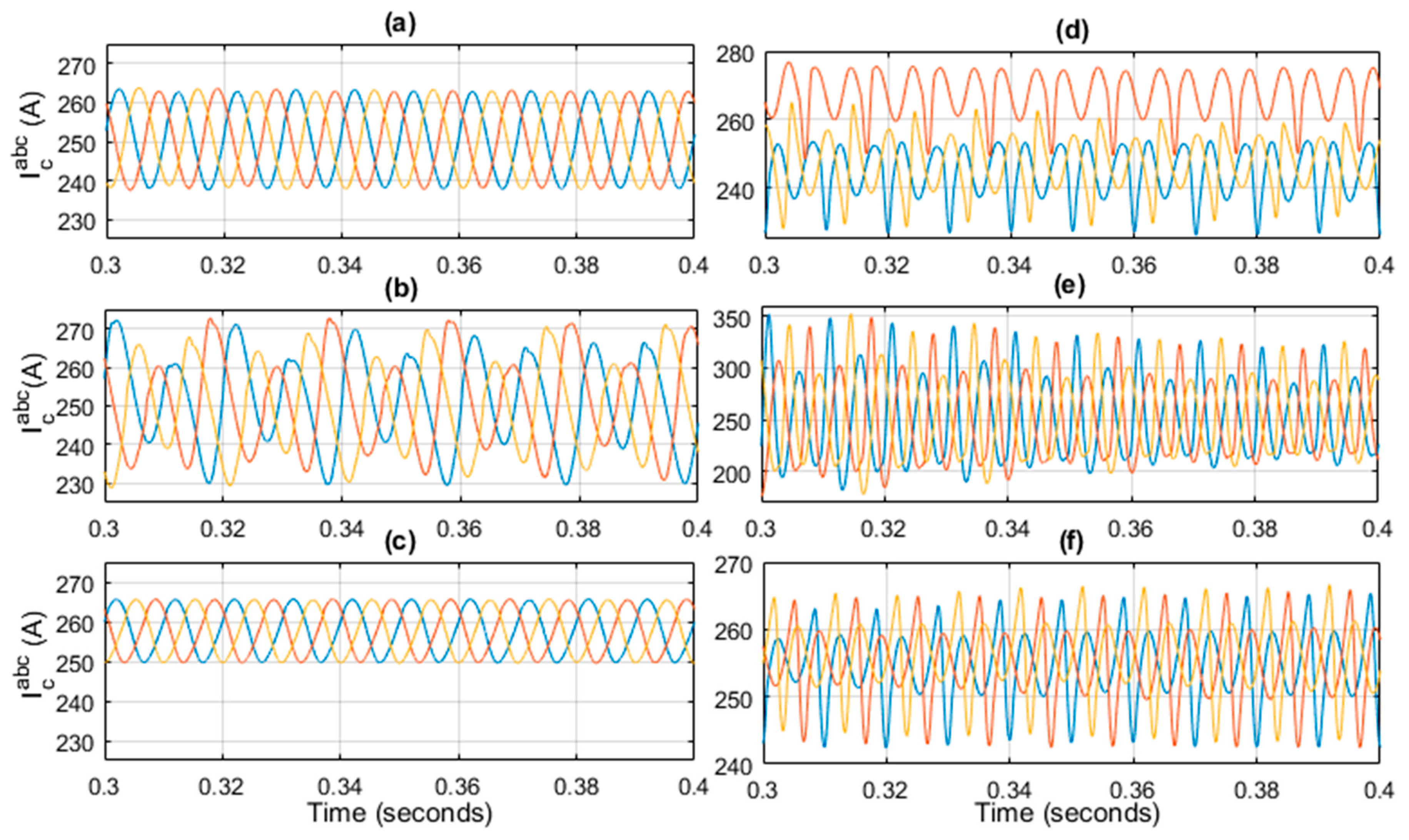
To check the effect of uncertainties on the control algorithm, the controller is subjected to parameter variation. The performance of the controller is checked for different values of the inductor, i.e., at half (L = 25 mH) and double (L = 100 mH) of the designed value. The response of the circulating current is given in Figure 10a–f. These figures are scaled to t = 0.5 s to show the transient response of the controlled variable. However, these figures are zoomed from t = 0.3 s to t = 0.4 s to show the steady-state response of the controlled variable as shown in Figure 11. Figure 10a–c show the response of the circulating current in case of the proposed controller. While Figure 10d–f show the response for the PR controller. Figure 10a,d show the response of the circulating current at nominal value (L = 50 mH). The response of the proposed controller shows that the circulating current is converging quickly as compared to the PR. The circulating current has the highest peak of 275 A as shown in Figure 10a while in the case of the PR, the current spike reaches to 400 A as shown in Figure 10d. Figure 10b,e show the response of the circulating current for L = 25 mH. Figure 10e shows a large variation of the circulating current as compare to Figure 10c. Similarly, Figure 10c has a better response than Figure 10d. The value of current increase beyond 400 A in case of PR controller. While the robust property of backstepping controller is converging the current to its reference value.

Moreover, by comparing the result of the same controller for different values of the inductor. The result is also satisfactory as shown in Figure 10a–c. Although the low value of the inductor (L = 25 mH) has some variation, its response is better than the PR controller. Similarly, by increasing the value of the inductor (L = 100 mH), the response of the circulating current becomes smooth, having a low amplitude of oscillation. But due to the large value of the inductor, the mean value of the current is shifted to 255 A instead of 250 A.

Similarly, by analyzing the zoomed response of both controller for different values of the inductor (L = 50 mH, L = 25 mH, L = 100 mH), it is concluded that backstepping controller has a better response to tackle parameter variation problems. Figure 11a–c shows that the amplitude of the circulating current changes from 260 A to 270 A in case of reducing the value of the inductor form L = 50 mH to 25 mH. However, the response of the circulating current is further smoothed by increasing the value of the inductor to 100 mH. While comparing backstepping to the PR, the amplitude of oscillation is lower in case of backstepping. The backstepping controller limits the amplitude of the circulating current to 270 A, while its peak touches the value of 350 A in case of the PR controller for 25 mH of the inductor value. Hence, by closely analyzing Figure 10 and Figure 11, it is concluded that the recursive Lyapunov-based backstepping controller has the ability to tackle the effect of parameter variations.

5. Conclusions and Future Work

This article presented control design architecture for controlling the internal dynamics of MMC. A backstepping controller was designed to control the internal dynamics, i.e., circulating current, capacitor voltage, and energy sum and energy difference. The design of the controller was based on Lyapunov stability function which ensured the asymptotic convergence of a closed-loop system. Moreover, the proposed control architecture enabled proper reference tracking, suppressed circulating current, and proper distribution of capacitor sum voltages in the desired SM. To validate the designed control architecture, the proposed backstepping controller was compared with a PR controller for results verification.

MATLAB/Simulink results of both the backstepping and PR controller shows that the backstepping controller exhibits better behavior than the PR controller. The backstepping controller converges the circulating current to the required value and the response time is improved in terms of its rise time and harmonic suppression. Moreover, the designed controller exhibited proper reference tracking of the circulating current, energy sum, and energy difference during transient and steady-state assuring a stable three-phase output voltage, while in the case of the PR controller, circulating current, energy sum, and energy difference were not converged properly to the required value. The proposed controller well-regulated the capacitor voltage in the desired SM without any fluctuation as compared to PR controller. Furthermore, the MMC parameters using backstepping controller are shown in

Table A1. Modular multilevel converter (MMC) parameters.

Parameters	Value	Symbols	Units
D.C Voltage	200	$V_{dc}$	kV
Grid Voltage (L-L)	100	$V_s$	kV
Output Peak Current	1	$I_s$	kA
Frequency	50	f	Hz
Sampling Frequency	10	fs	kHz
Number of levels	12	N	-
Arm Inducatnce	50	L	mH
Arm Resistance	1.57	R	Ω
Submodule Capcitance	0.45	C	mF

of Appendix A.

Moreover, in the near future, the proposed control structure for internal dynamics results will be validated using FPGA, DSPACE or DSP TMS320F28335 board (Delfino Texas Instrument, TX, USA). Additionally, new control schemes, i.e., exact feedback linearization and h-infinity, will be designed and compared with the proposed backstepping control scheme.

References

1. Martinez-Rodrigo, F.; Ramirez, D.; Rey-Boue, A.B.; De Pablo, S.; Herrero-de Lucas, L.C. Modular Multilevel Converters: Control and Applications. Energies 2017, 10, 1709. [Google Scholar] [CrossRef]
2. Debnath, S.; Qin, J.; Bahrani, B.; Saeedifard, M.; Barbosa, P. Operation, Control, and Applications of the Modular Multilevel Converter: A Review. IEEE Trans. Power Electron. 2015, 30, 37–53. [Google Scholar] [CrossRef]
3. Hagiwara, M.; Nishimura, K.; Akagi, H. A Medium-Voltage Motor Drive With a Modular Multilevel PWM Inverter. IEEE Trans. Power Electron. 2010, 25, 1786–1799. [Google Scholar] [CrossRef]
4. Ishfaq, M.; Uddin, W.; Zeb, K.; Khan, I.; Ul Islam, S.; Adil Khan, M.; Kim, H.J. A New Adaptive Approach to control circualting and output current of Modular Multilevel Converter. Energies 2019, 12, 1118. [Google Scholar] [CrossRef]
5. Nami, A.; Liang, J.; Dijkhuizen, F.; Demetriades, G.D. Modular Multilevel Converters for HVDC Applications: Review on Converter Cells and Functionalities. IEEE Trans. Power Electron. 2015, 30, 18–36. [Google Scholar] [CrossRef]
6. Kouro, S.; Malinowski, M.; Gopakumar, K.; Pou, J.; Franquelo, L.G.; Wu, B.; Rodriguez, J.; Perez, M.A.; Leon, J.I. Recent Advances and Industrial Applications of Multilevel Converters. IEEE Trans. Ind. Electron. 2010, 57, 2553–2580. [Google Scholar] [CrossRef]
7. Du, S.; Dekka, A.; Wu, B.; Zargari, N. Modular Multilevel Converters: Analysis, Control, and Applications; John Wiley & Sons: Hoboken, NJ, USA, 2017. [Google Scholar]
8. Lacerda, V.A.; Coury, D.V.; Monaro, R.M. Proportional-resonant controller applied to modular multilevel converter for HVDC systems. In Proceedings of the 2018 Simposio Brasileiro de Sistemas Eletricos (SBSE), Niteroi, Brazil, 12–16 May 2018; pp. 1–6. [Google Scholar]
9. Martinez-Rodrigo, F.; de Pablo, S.; Herrero-de Lucas, L.C. Current control of a modular multilevel converter for HVDC applications. Renew. Energy 2015, 83, 318–331. [Google Scholar] [CrossRef]
10. Hagiwara, M.; Akagi, H. Control and Experiment of Pulsewidth-Modulated Modular Multilevel Converters. IEEE Trans. Power Electron. 2009, 24, 1737–1746. [Google Scholar] [CrossRef]
11. Tu, Q.; Xu, Z.; Xu, L. Reduced Switching-Frequency Modulation and Circulating Current Suppression for Modular Multilevel Converters. IEEE Trans. Power Deliv. 2011, 26, 2009–2017. [Google Scholar]
12. Bahrani, B.; Debnath, S.; Saeedifard, M. Circulating Current Suppression of the Modular Multilevel Converter in a Double-Frequency Rotating Reference Frame. IEEE Trans. Power Electron. 2016, 31, 783–792. [Google Scholar] [CrossRef]
13. Lizana, R.; Perez, M.A.; Arancibia, D.; Espinoza, J.R.; Rodriguez, J. Decoupled Current Model and Control of Modular Multilevel Converters. IEEE Trans. Ind. Electron. 2015, 62, 5382–5392. [Google Scholar] [CrossRef]
14. Li, Z.; Wang, P.; Chu, Z.; Zhu, H.; Luo, Y.; Li, Y. An Inner Current Suppressing Method for Modular Multilevel Converters. IEEE Trans. Power Electron. 2013, 28, 4873–4879. [Google Scholar] [CrossRef]
15. Yang, S.; Wang, P.; Tang, Y.; Zagrodnik, M.; Hu, X.; Tseng, K.J. Even-harmonic repetitive control for circulating current suppression in Modular Multilevel Converters. In Proceedings of the 2016 IEEE Applied Power Electronics Conference and Exposition (APEC), Long Beach, CA, USA, 20–24 March 2016; pp. 3591–3597. [Google Scholar]
16. He, L.; Zhang, K.; Xiong, J.; Fan, S. A Repetitive Control Scheme for Harmonic Suppression of Circulating Current in Modular Multilevel Converters. IEEE Trans. Power Electron. 2015, 30, 471–481. [Google Scholar] [CrossRef]
17. Zhang, M.; Huang, L.; Yao, W.; Lu, Z. Circulating Harmonic Current Elimination of a CPS-PWM-Based Modular Multilevel Converter With a Plug-In Repetitive Controller. IEEE Trans. Power Electron. 2014, 29, 2083–2097. [Google Scholar] [CrossRef]
18. Barnklau, H.; Gensior, A.; Rudolph, J. A Model-Based Control Scheme for Modular Multilevel Converters. IEEE Trans. Ind. Electron. 2013, 60, 5359–5375. [Google Scholar] [CrossRef]
19. Ben-Brahim, L.; Gastli, A.; Trabelsi, M.; Ghazi, K.A.; Houchati, M.; Abu-Rub, H. Modular Multilevel Converter Circulating Current Reduction Using Model Predictive Control. IEEE Trans. Ind. Electron. 2016, 63, 3857–3866. [Google Scholar] [CrossRef]
20. Vatani, M.; Bahrani, B.; Saeedifard, M.; Hovd, M. Indirect Finite Control Set Model Predictive Control of Modular Multilevel Converters. IEEE Trans. Smart Grid 2015, 6, 1520–1529. [Google Scholar] [CrossRef] [Green Version]
21. Riar, B.S.; Geyer, T.; Madawala, U.K. Model Predictive Direct Current Control of Modular Multilevel Converters: Modeling, Analysis, and Experimental Evaluation. IEEE Trans. Power Electron. 2015, 30, 431–439. [Google Scholar] [CrossRef]
22. Qin, J. Predictive control of a modular multilevel converter for a back-to-back HVDC system. IEEE Trans. Power Deliv. 2012, 27, 1538–1547. [Google Scholar]
23. Yang, S.; Wang, P.; Tang, Y. Feedback Linearization-Based Current Control Strategy for Modular Multilevel Converters. IEEE Trans. Power Electron. 2018, 33, 161–174. [Google Scholar] [CrossRef]
24. Harnefors, L.; Antonopoulos, A.; Ilves, K.; Nee, H.P. Global Asymptotic Stability of Current-Controlled Modular Multilevel Converters. IEEE Trans. Power Electron. 2015, 30, 249–258. [Google Scholar] [CrossRef]
25. Bergna, G.; Garces, A.; Berne, E.; Egrot, P.; Arzande, A.; Vannier, J.-C.; Molinas, M. A Generalized Power Control Approach in ABC Frame for Modular Multilevel Converter HVDC Links Based on Mathematical Optimization. IEEE Trans. Power Deliv. 2014, 29, 386–394. [Google Scholar] [CrossRef]
26. Sharifabadi, K.; Harnefors, L.; Nee, H.P.; Norrga, S.; Teodorescu, R. Dynamics and Control. In Design, Control and Application of Modular Multilevel Converters for HVDC Transmission Systems; John Wiley & Sons, Ltd.: Chichester, UK, 2016; pp. 133–213. [Google Scholar]
27. Ahmad, N.; Angquist, L.; Norrga, S.; Antonopoulos, A.; Harnefor, L.; Nee, H.P. A computationally efficient continous model for modular multilevel converter. IEEE J. Emerg. Sel. Top. Power Electron. 2014, 2, 1139–1148. [Google Scholar] [CrossRef]
28. Liu, J. Backstepping control with RBF. In Radial Basis Function (RBF) Neural Network Control for Mechincal Systems Design, Analysis and Matlab Simulation; Springer: Berlin/Heidelberg, Germany, 2013; pp. 251–291. [Google Scholar]
29. Zhou, J.; Wen, C. Adaptive backstepping control. In Adaptive Backstepping Control of Uncertain Systems Nonsmooth Nonlinearities, Interaction or Time-Variations; Springer: Berlin/Hiedelberg, Germany, 2007; pp. 9–25. [Google Scholar]
Figure 1. Grid connected modular multilevel converter (MMC).
Electronics 08 00456 g001
Figure 2. Equivalent circuit of MMC.
Electronics 08 00456 g002
Figure 3. Leg level model of MMC.
Electronics 08 00456 g003
Figure 4. Structure of design controller.
Electronics 08 00456 g004
Figure 5. Circulating current (a) Proposed controller with constant reference; (b) Proportional resonant (PR) controller with constant reference; (c) Proposed controller with stepped reference; (d) PR controller with stepped reference.
Electronics 08 00456 g005
Figure 6. Energy difference (a) Proposed controller with constant reference; (b) PR controller with constant reference; (c) Proposed controller with stepped reference; (d) PR controller with stepped reference.
Electronics 08 00456 g006
Figure 7. Energy sum (a) Proposed controller with constant reference; (b) PR controller with constant reference; (c) Proposed controller with stepped reference; (d) PR controller with stepped reference.
Electronics 08 00456 g007
Figure 8. Upper arm capacitor voltage (a) Proposed controller; (b) PR controller.
Electronics 08 00456 g008
Figure 9. Converter output voltage (a) Proposed controller; (b) PR controller.
Electronics 08 00456 g009
Figure 10. Circulating current at (a) L = 50 mH in case of proposed controller; (b) L = 25 mH in case of proposed controller; (c) L = 100 mH in case of proposed controller; (d) Nominal value of Inductor in case of the PR; (e) L = 25 mH in case of the PR; (f) L = 100 mH of nominal inductor value in case of the PR.
Electronics 08 00456 g010
Figure 11. Circulating current at steady state (ac) Backstepping controller; (df) PR controller; (a,d) L = 50 mH; (b,e) L = 25 mH; (c,f) L = 100 mH.
Electronics 08 00456 g011