Magnetic Switching of a Stoner-Wohlfarth Particle Subjected to a Perpendicular Bias Field

Abstract

Characterized by uniaxial magnetic anisotropy, the Stoner-Wohlfarth particle experiences a change in magnetization leading to a switch in behavior when tuned by an externally applied field, which relates to the perpendicular bias component (h_perp) that remains substantially small in comparison with the constant switching field (h₀). The dynamics of the magnetic moment that governs the magnetic switching is studied numerically by solving the Landau-Lifshitz-Gilbert (LLG) equation using the Mathematica code without any physical approximations; the results are compared with the switching time obtained from the analytic method that intricately treats the non-trivial bias field as a perturbation. A good agreement regarding the magnetic switching time (t_s) between the numerical calculation and the analytic results is found over a wide initial angle range (0.01 < θ₀ < 0.3), as h₀ and h_perp are 1.5 × K and 0.02 × K, where K represents the anisotropy constant. However, the quality of the analytic approximation starts to deteriorate slightly in contrast to the numerical approach when computing t_s in terms of the field that satisfies h_perp > 0.15 × K and h₀ = 1.5 × K. Additionally, existence of a comparably small perpendicular bias field (h_perp << h₀) causes t_s to decrease in a roughly exponential manner when h_perp increases.

1. Introduction

Growing research attention has been paid to controlling the magnetization reversal in ferromagnetic multilayer configurations in the past two decades [1,2,3,4,5,6]. To primitively describe the magnetic dynamics of single-domain ferromagnets [7], it appears necessary to revisit the Stoner-Wohlfarth (SW) model that was originally proposed by E. C. Stoner and E. P. Wohlfarth in 1948 [8]. Based on their early work, many additional extensions [9,10,11] of the simplified SW model have undergone intensive investigation motivated by the current progress in computational technology applied to solid-state physics. The concept of “magnetic switching” plays a key role in the reading and writing of information and monitoring the magnetization in magnetic material. In our study, the time-dependent magnetization vector of a particle satisfying the SW model requirement is examined and associated with the applied torque (due to externally applied magnetic fields) that causes magnetic moment reversal to occur. For the crucial importance of investigating the dynamical behavior of magnetization in a SW particle modulated by a significantly small bias field, one notices that discerning how to efficiently manipulate the magnetic state of a primitive single-domain ferromagnet is key to the development of ferromagnetic spintronics. Specifically, there exists two major aspects that motivate our current study. First, the local modulation of magnetization being done by tuning the magnitude of the bias magnetic field should be completed in a more efficient manner than the traditional method which uses electric fields to store information in the computer memory named “dynamic random-access memory” (DRAM), because information storage in such a conventional method is transient and easily lost when turning off the computer. Therefore, newer way of memorizing information such as “magnetic random-access memory” (MRAM), which uses long-lasting ferromagnetism and ferroelectricity, is strongly desired. Second, increasing the magnetic switching rates is required by the disk speed and recorded density with respect to the physical equipment in computer memory part. Accordingly, ferromagnetic materials have become increasingly essential and demonstrate many promising practical applications including nano-scale memory devices and magnetic field probes [12,13,14].

At present, our work discusses the switching behavior of a Stoner-Wohlfarth particle (sometimes called single-domain magnetic grain) for the instance when the external fields that involve the driving field (h₀) along with the small bias field (h_perp) are simultaneously present. Among the results, the time it takes for the magnetization vector to experience an angle change, which is a bit smaller than π/2, and how the bias field strength (or initial angle parameter) effects the switching time are extensively explored in this paper.

There exist many computational techniques that can be used to reveal the magnetic dynamics governed by the Landau-Lifshitz-Gilbert (LLG) equation [15], which was developed after the Landau-Lifshitz (LL) equation [16,17]. In general, many codes utilizing Monte Carlo methods, fast Fourier transformations, etc., have been utilized to obtain a numerical simulation of the magnetization occurring in actual magnetic grains, as well as the time evolution of other physical quantities, namely, the vortex profile, dipole–dipole interaction, etc. [18,19,20]. In addition to these programs, which aim to acquire the time evolution of magnetic quantities without any physical approximations, one learns that an analytic solution within the framework of the LLG equation provides another valid and effective method to interpret the actual magnetic behavior of various systems [21,22,23], including our study, which uses appropriate analytic approximations, such as the perturbation theory. Specifically, for our work, we compare the magnetic switching time gained using two different computational methods (numerical and analytical approaches) and examine the apparent agreement (or slight discrepancy) between these approaches.

This paper is structured as follows. We briefly introduce the fundamental model (LLG equation) used to explain the time evolution of the magnetic moment in the context of the Bloch equation along with the LL equation, with the goal of establishing the analytic approach (involving appropriate approximations) that applies to the switching time computation. Then, the interplay of the magnetic driving field and the perpendicular bias field occurring in a Stoner-Wohlfarth particle is reviewed and contrasted with our calculated results, which suggest that magnetic switching can be effectively tuned using a significantly small bias field. In the discussion section, the magnetic switching time in the case of axial symmetry (no bias field), as well as in the case of a small perpendicular bias field, is analytically examined, exhibiting fair agreement with the numerically obtained data.

2. Model

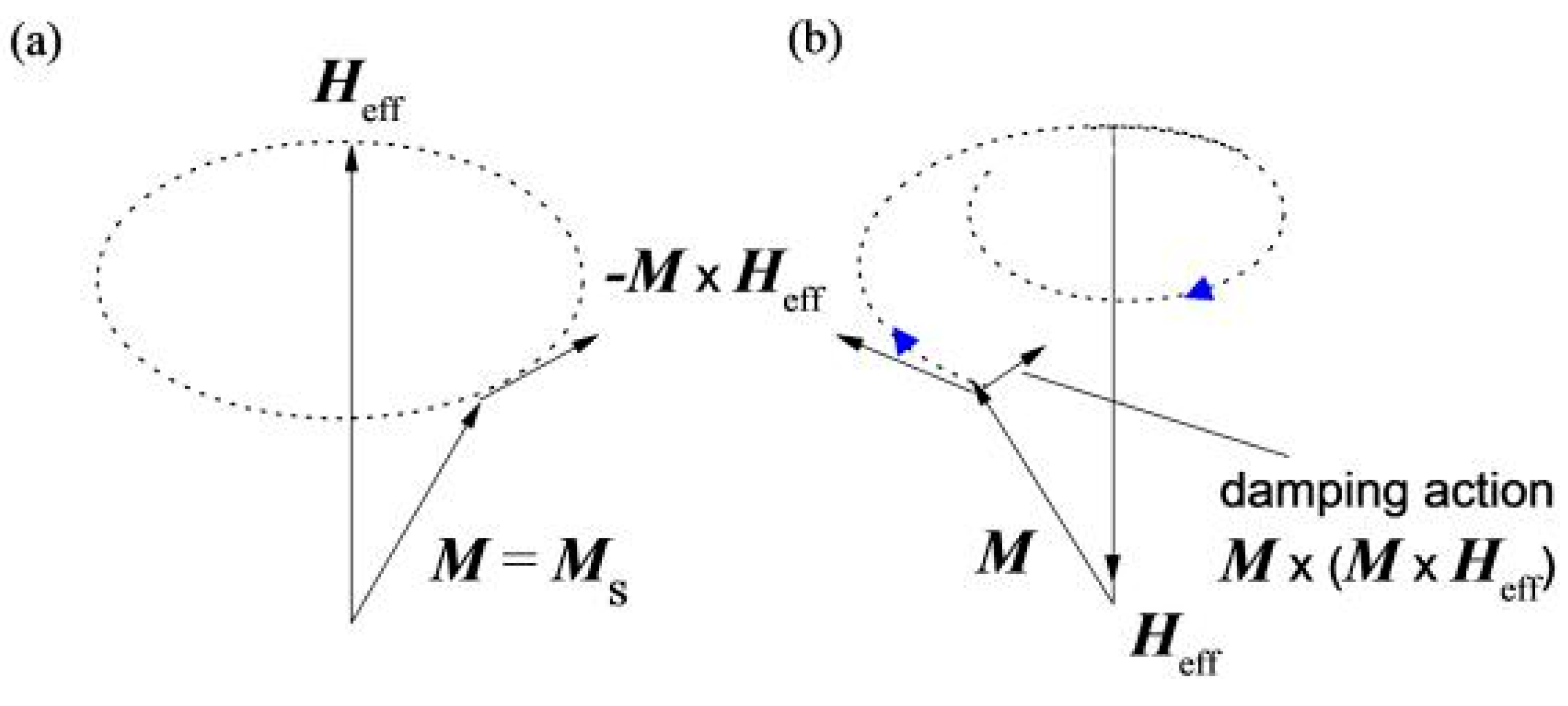
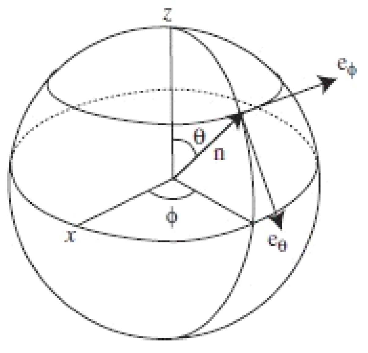
2.1. Magnetic Moment Dynamics

For the purpose of characterizing the magnetic dynamics that govern the time evolution of the magnetization vector M, the Bloch equation [24] was initially proposed via relation dM/dt = γ₀ × M × H, where γ₀ described the gyromagnetic ratio while H represented the external field. Then, Landau and Lifshitz extended the Bloch equation to the parameter M subjected to the effective field (H_eff), which arose from the negative functional magnetization derivative with respect to the magnetic energy (−δE_m/δM), as well as the dissipation terms, which were related to the loss and relaxation processes in ferromagnetic materials. Consequently, the derived Landau-Lifshitz (LL) equation is as follows:

dM/dt = −γ₀ × M × H_eff + λ × γ₀/|M| × M × (M × H_eff)

(1)

where Landau and Lifshitz assumed that the dissipation was described by a nonlinear term (second term in Equations (1)) of the form restricted by the same effective field, while introducing the coefficient λ and taking into account the gyromagnetic ratio γ₀. The first term on the right-hand side (RHS) of Equation (1) describes the dissipationless motion of the moment. Notice that the LL equation conserves the magnetic moment |M|= (M·× M)^1/2 and takes the scalar product of M and all terms, except for the nonlinear term appearing in Equation (1), which leads to M·(dM/dt) = 0. Therefore, one finds that |M| = M_s = a constant, where M_s represents the magnitude of the saturation magnetization under the circumstance of a negligible second term in the RHS of Equation (1). This can be illustrated with the example of a uniaxial anisotropic magnet placed into an external field (H_eff) directed along the same axis. The left panel of the figure below shows that without dissipation, the moment performs a circular motion along the parallels of a unit sphere, so that |M| = a constant is maintained. In the absence of dissipation, the precession of the moment persists for an infinitely long time and is shown in the left panel of Figure 1.

In real experiments, dissipation losses play a crucial role in regulating the dynamics of the moment. Even a small variation in the dissipation torque can cause the moment to change significantly. As the right panel of Figure 1 shows, the dissipation torque is the only torque that actually pushes M toward the minimum magnetic energy, resulting in a magnetization trajectory that is on the spherical surface due to its constant module |M|, and eventually precesses to the direction which is almost aligned along the −H_eff field direction.

The divergence problem arises when significantly large dissipation losses (λ >> 1) are available in the LL equation. To conquer this trouble, Gilbert modified the dissipation term by taking a damping quantity of the form α × M_s⁻¹ × M × (dM/dt) into account. α acts as the Gilbert damping coefficient. Consequently, the motion of a magnetic moment in the context of a redefined damping factor along with effective field was mathematically given by the so-called Landau-Lifshitz-Gilbert (LLG) equation:

dM/dt = −γ × M × H_eff + α × M_s⁻¹ × M × (dM/dt)

(2)

where γ is another gyromagnetic ratio, and α turns out to be the Gilbert damping parameter. It appears straightforward to verify that we can retrieve the LL equation format from the LLG counterpart. Taking the cross product of the left-hand side (LHS) of Equation (2) with M, and using M norm conservation (M·× (dM/dt) = 0), one can obtain the following:

M × dM/dt = −γ × M × (M × H_eff) + α × M_s × (dM/dt)

(3)

Notice that M_s represents the magnitude of the moment vector M. Inserting M × (dM/dt), which roots from the LHS of Equation (3) into Equation (2), one eventually obtains the following:

dM/dt = −γ × (1 + α²)⁻¹ × (M × H_eff) − α × γ × M_s⁻¹ × (1+α²)⁻¹ × M × (M × H_eff)

(4)

Here, one may identify γ₀ as γ × (1 + α²)⁻¹ and λγ₀/|M| as α × γ × M_s⁻¹ × (1+α²)⁻¹, then both equations (LL and LLG) become identical.

The next step was to transform Equation (4) into the dimensionless form. Dividing both sides of Equation (2) by γ × M_s gave rise to the below expression:

(γ × M_s)⁻¹ × dM/dt = −M_s⁻¹ × M × H_eff + (α × γ⁻¹ × M_s⁻²) × M × (dM/dt)

(5)

with the following definitions: n = M/M_s and h_eff = γ × H_eff, one can rearrange Equation (5) to obtain the dimensionless equation: dn/dt = −n × h_eff + α × n × dn/dt. Then, taking the cross product of n and the expression involving dn/dt, one can finally determine the following:

(1 + α²) × dn/dt = −n × h_eff + α × h_eff

(6)

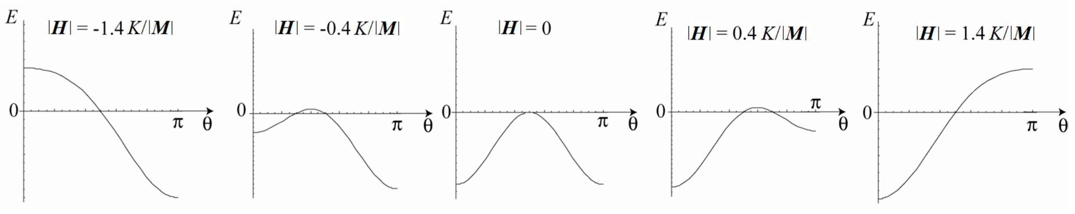
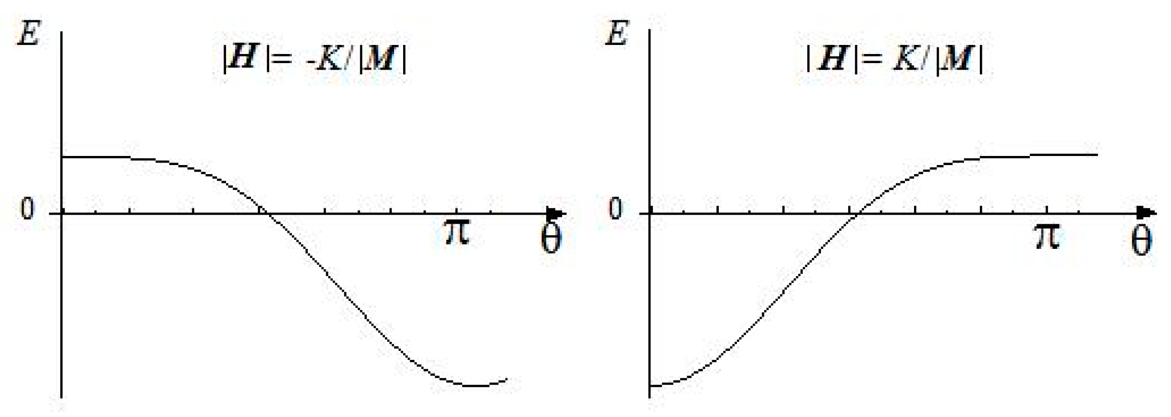
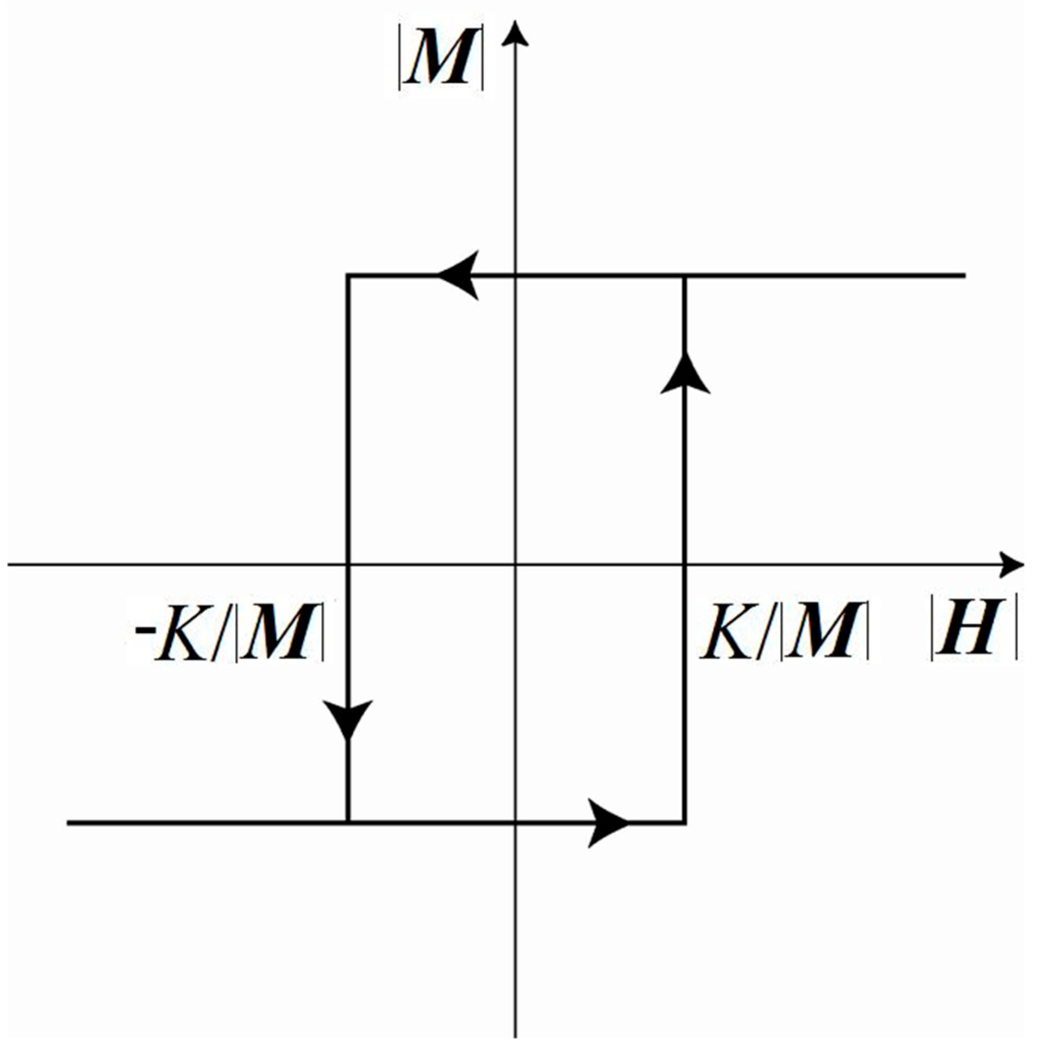
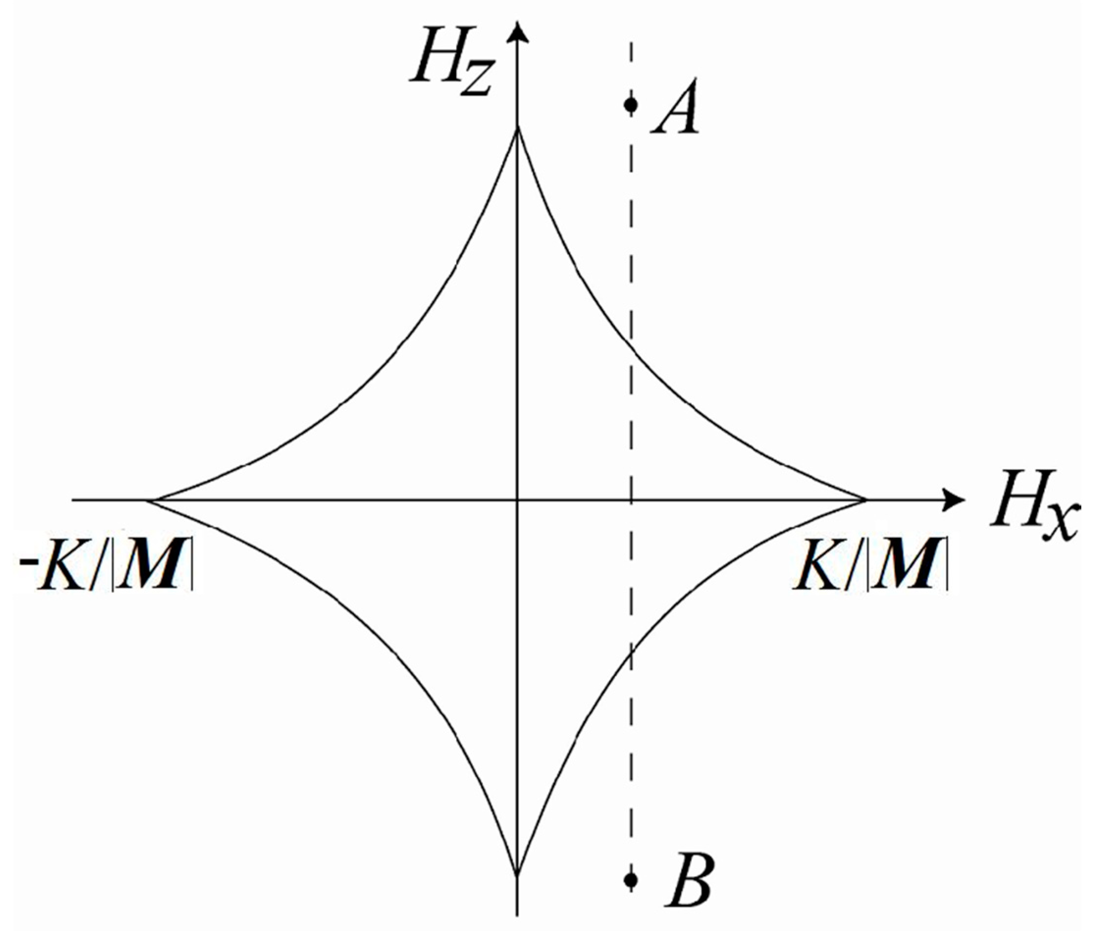
2.2. Stoner-Wohlfarth Model

To understand how the presence of magnetic anisotropy leads to the existence of preferred directions for moment M, one realizes that the origin of anisotropy energy E_A stems from two factors: The crystalline anisotropy ultimately caused by the spin–orbit interactions in the material [25] and the shape anisotropy caused by the energy of the fields induced by the magnetic moment [26]. The properties of these two types of energy remain complex in multi-domain samples, while the anisotropy energy E_A(n) of a single-domain case has the uniaxial form:

E_A = −1/2 × K × (n × z)²

(7)

where K is the anisotropy constant that stays positive, and z denotes a unit vector along the z-axis. The minimum of the anisotropy is achieved for n = +z or n = −z in the context of a positive K, while the z-axis here is defined as the easy axis of the magnetic material. Considering a single-domain magnet that is placed into an external magnetic field H, one notices that an additional contribution to the energy that is equivalent to (–M·× H) arises. Hence, the total energy is consequently defined by the following:

E_A = −1/2 × K × (n × z)² − M·× H

(8)

In terms of spherical angles, θ and φ are commonly used to parameterize the unit vector n = (sinθcosφ, sinθsinφ, cosθ), and the total energy E_A is rewritten based on the re-expressed component (n_x, n_y, n_z) as the following:

E_A = −1/2 × K × cos²θ − |M| × |H| × cosθ

(9)

Such energy, which depends solely on angle θ, can now be plotted as a series of E(θ) graphs in the following (see Figure 2). The qualitative shape of each diagram appears to be different relying on the value of |H| = H_z/cosθ.

As shown in the figure above, for −K/|M| < |H| < K/|M|, there are two minima of energy in the angle interval (0, π), while for |H| > K/|M| (or |H| < −K/|M|) there exists only one minimum within the same parameter range. If one initially sets the field to a positive value, for instance, |H| > K/|M|, the available energy minimum can only be acquired at θ = 0, which corresponds to the moment pointing in the +z direction. By decreasing the field until it eventually approaches its negative counterpart (from |H| = 1.4 × K/|M| to |H| = −1.4 × K/|M| in Figure 2), one can switch the moment from up (cosθ = 1) to down (cosθ = −1). The switching behavior indeed occurs when the energy minimum in the curves at θ = 0 disappears.

It is apparent to deduce from Equation (9) that this critical phenomenon can be numerically captured at the field value |H| = −K/|M|. Continuing to tune the field toward −1.4 × K/|M|, one finds that the moment abruptly jumps into a state with θ = π, (i.e., being directed along −z). In other words, the moment stays in the downstate situation. If the field is increased up from a negative value (e.g., |H| < −K/|M|), the moment remains in the minimum state (θ = π) until the field reaches the value of |H| = +K/|M|, at which point this minimum configuration disappears and the moment eventually jumps back into the “new” stable minimum at θ = 0. Consequently, Figure 3 shows the magnetic energy E as a function of angle θ for the special cases where |H| = ±K/|M|. The |M|(|H|) dependence has a form shown below (Figure 4).

It is observed that this magnetic hysteresis has a rectangular hysteresis loop, and its width (or coercive field) is K/|M|. A more complicated situation where H has two nonzero components given by H = (H_x, 0, H_z) is of great significance and is analogous to a Stoner-Wohlfarth particle. It is assumed that the longitudinal component H_z stays extremely larger than the perpendicular component H_x which is free to be tuned and is defined as a bias field for later discussion. Currently, the study of the switching behavior of a uniaxial magnet in the presence of a bias field, in addition to a longitudinal field, has been attracting increasing attention [27,28]. For the purpose of seeking the critical value of H_x at which the switching occurs supposing that H_z is fixed, the functional dependence H_z(H_x) describing interplay of these two critical fields is plotted in the following figure and given mathematically as [11,29,30,31]:

H_z^2/3 + H_x^2/3 = (K/|M|)^2/3

(10)

Depicting the above relation between the bias field and the fixed field leads to the resulting diagram, which is referred to as the asteroid curve, in which the dashed line in Figure 5 shows how the total field H changes when H_z varies itself at a fixed value of H_x.

It is assumed that the longitudinal field H_z is abruptly tuned from the field point A to the one corresponding to the field at point B, as a function of a constant H_x. This is due to the fact that, tangents to the asteroid give rise to magnetization directions with external energy. For a system with a uniaxial anisotropy, the tangents that are closer to the easy axis can result in stable solutions (minimum energy configuration). Specifically, in the initial state A, the magnetic moment is pointing mostly in the +z direction because of a slight deviation from +z due to the presence of a nonzero, yet very small, H_x (H_x << K/|M|). After an abrupt change of H_z to the value confined at state B, the “up equilibrium” no longer exists, and the moment rotates to the “down equilibrium”; however, the moment is directed almost along −z (again, a small deviation from −z is present due to H_x). An important characteristic of this switching process is numerically manifested by the switching time t_s, since such parameter plays a crucial role in technological applications, pertinent to which the single-domain particles are used to store digital information. In other words, a smaller switching time means information is written into memory equipment faster. In this paper, the switching time of a uniaxial Stoner-Wohlfarth particle at a significantly small bias field was investigated by virtue of an analytical method along with a numerical calculation.

3. Results and Discussion

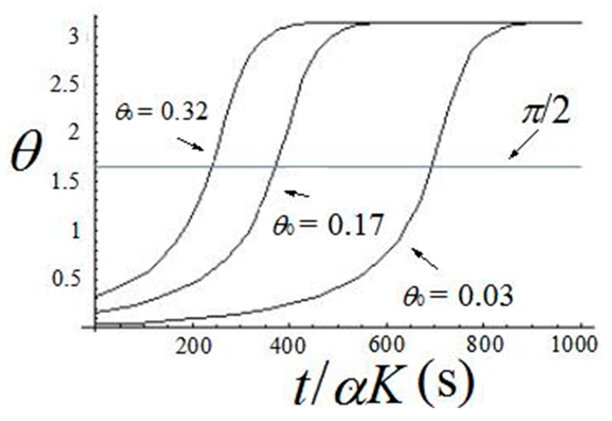
3.1. Switching Behavior under Axial Symmetry

Before performing practical calculations to determine the magnetic switching time of an SW particle subjected to an additional bias field, it was necessary to convert the derived vector Equation (6) within the small damping approximation (α << 1) to a system of two scalar equations on (θ, φ). Figure 6 introduces the two vectors e_θ and e_φ, both of which are tangent to the unit sphere.

By differentiating the expressions n = (sinθcosφ, sinθsinφ, cosθ), e_θ = (cosθcosφ, cosθsinφ, −sinθ) and e_φ = (−sinφ, cosφ, 0) with respect to time t while making use of the right-hand coordinate system, including a standard unit basis (e.g., e_θ × e_φ = n), one can transform Equation (6) into the form:

(dθ/dt) × e_θ + (dφ/dt) × sinθe_φ = (əE_SW/əθ) × e_φ − sin⁻¹θ × (əE_SW/əφ) × e_θ +
α × ((dθ/dt) × e_φ − (dφ/dt) × sinθe_θ)

(11)

where E_SW is identified as the energy pertaining to an SW particle of interest, and the LHS of Equation (6) is approximated as dn/dt. Next, by equating the coefficients pertinent to both tangent vectors appearing in the LHS of Equation (11) and rearranging the appropriate time derivatives with respect to the angles, one finally finds the following:

dθ/dt = −sin⁻¹θ × (əE_SW/əφ) − α × (əE_SW/əθ)

(12)

dϕ/dt = sin⁻¹θ × (əE_SW/əθ) − α × sin⁻²θ × (əE_SW/əφ)

(13)

We now investigated the switching behavior in the case of axial symmetry (H_x = 0) in the context where the magnetic energy was assumed to depend solely on the θ parameter (E(θ) = −1/2 × K × cos²θ − |M| × |H| × cosθ). Therefore, two independent equations associated with the angle variables are given:

dθ/dt = −α × sinθ × (K × cosθ + h_z)

(14)

Here, conducting an integration of Equation (14) over θ and t subjected to a provided initial angle θ₀ ≡ θ(t = 0) was apparently responsible for resolving the magnetic switching time. The switching field h_z is denoted as H_z × |M|. Suppose one initiates with a magnetic moment positioned close to the +z direction and applies a negative magnetic field −H₀ (aligned along −z) sufficient to induce a switch. A representation of the dependence of θ on t (in the unit of α × K) according to the model described mathematically in Equation (14) is shown in Figure 7. As the switching process progressed, different curves reflecting angle θ (given in the unit of radian) versus time, arose due to the distinct values of θ₀. By the end of the switching process, the moment had approached the −z direction, and the angle θ approached π.

Two features of this graph are important for us to revisit. First, the switching behavior occurred much faster for larger values of θ₀. Second, each trajectory path describing the time-dependent angle approached a final value that was sufficiently close to π in an exponential form. That is, the curve formally took a comparably long time to achieve the entire variation process (from θ < 0.5 to θ = π). To efficiently define a finite switching time, it is customary to select a cutoff angle θ_s and to calculate the corresponding time t_s it takes to reach that angle. Figure 7 shows that the switching behavior confined in the angle range of 0 to π exists over a relatively short time interval. Prior to this interval, the angles inside different curves were close to θ₀, and beyond this interval, the angles remained close to π. The midpoint for the time of this interval was roughly located at θ_s = π/2. This explains why it made sense to select π/2 as a cutoff angle. Such a critical angle value has been frequently used in the literature [32,33]. Additionally, it is noted that at the same time (t = t_s), the projection moment M_z had reached zero.

Continuing with the exact analytic expression of Equations (12) and (14), we resolved the analytic solution to obtain the switching time of the magnetic particle in the context of axial symmetry by means of integration using separation of variables. By integrating Equation (14) over time parameter t as well as angle θ while imposing the condition θ(t = 0) = θ₀, the analytic solution finally becomes the following:

t_s ≡ t⁽⁰⁾_s(θ₀) = −(1/2) × α⁻¹ × ((K + h_z)⁻¹ × In(h_z × (1 − cosθ₀) × (K × cosθ₀ + h_z)⁻¹) +
(K − h_z)⁻¹ × In(h_z × (1 + cosθ₀) × (K × cosθ₀ + h_z)⁻¹))

(15)

One crucial thing about the understanding of the initial angle θ₀ requires emphasis. The switching time t⁽⁰⁾_s(θ₀) ultimately approached zero once θ₀ was close to π/2. Additionally, this conclusion was certainly consistent with common sense. A similar expression concerning Equation (15) was derived in another report, in particular for the case where K = 0, and for an arbitrary K [34].

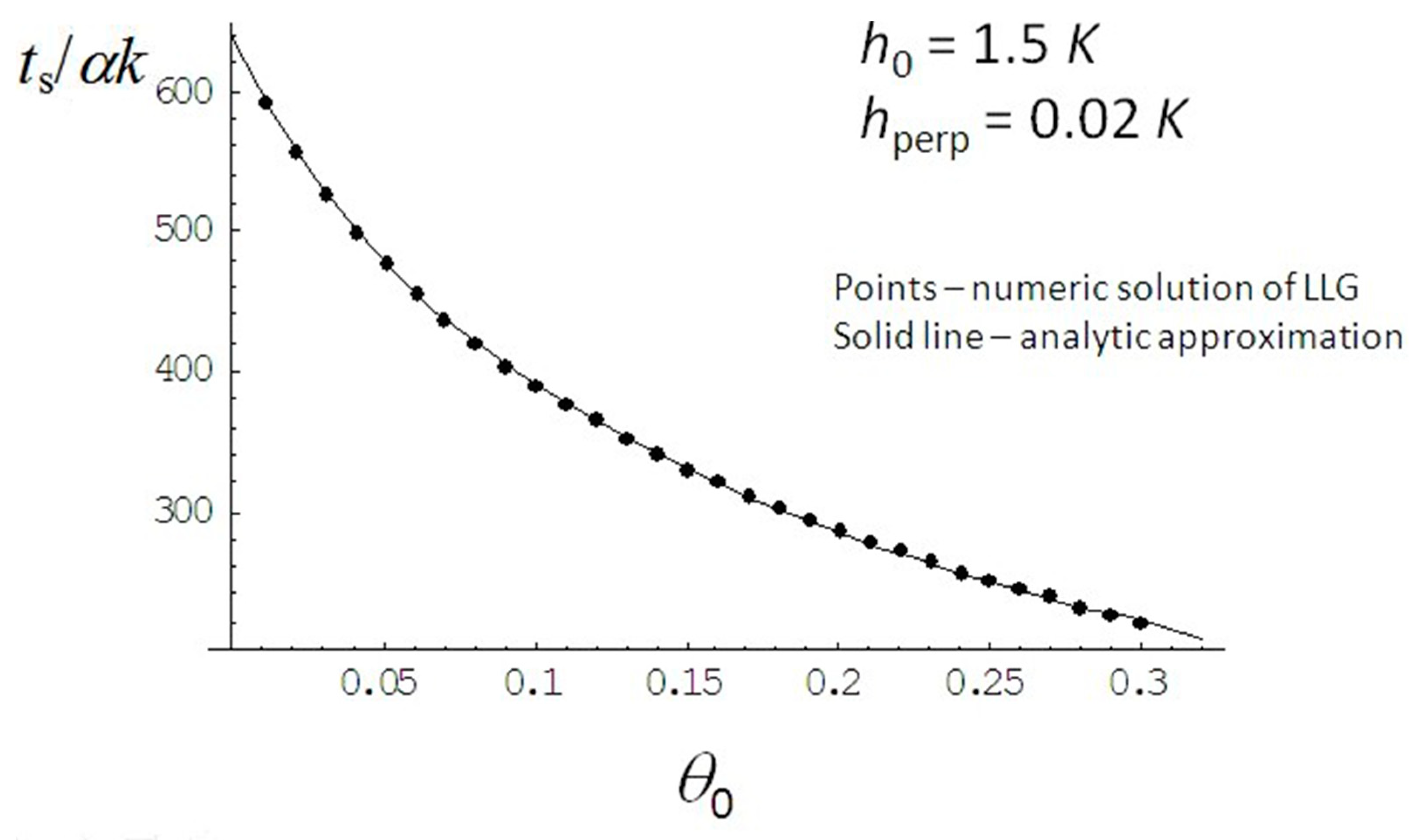
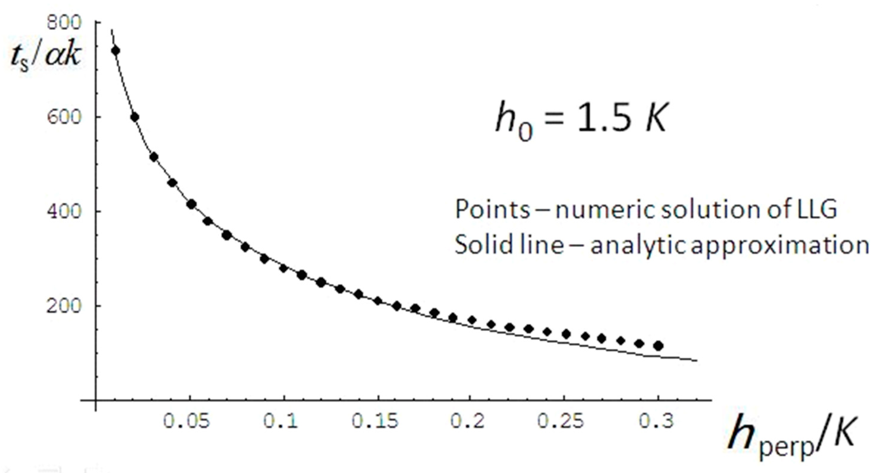
3.2. Switching Behavior of an SW particle in a Small Perpendicular Bias Field

In the presence of the switching field H₀ pointing in the negative z-axis and the bias field H_perp pointing in the positive x-axis, the energy density of a Stoner-Wohlfarth particle is expressed as the following:

E_sw = −1/2 × K × cos²θ − |M| × |H_perp| × sinθ × cosϕ − |M| × |H₀| × cosθ

(16)

Here, the switching field and the bias field were also recognized as h_perp = H_perp × |M| and h_z = H₀ × |M|. If the bias field H_perp was significantly small (h_perp = |h_perp| << h_z = |h_z|), one can hope to find an analytic approximation to obtain the switching time by taking such a bias field into account as a small perturbation. Similar reports addressing the precessional magnetization switching under a biased perpendicular anisotropy can be found in [35,36]. The result can be formulated as follows. Combining Equation (12) and (15), one notes that the magnetic switching time was identified from the following expression after integration over angle θ and time t, respectively:

dθ/dt = −α × sinθ × (K × cosθ + h_z) − h_perp × sinϕ

(17)

Treating the −h_perp × sinϕ term as a perturbation and depending on the previously obtained switching time appearing in Equation (15), the determination of t⁽⁰⁾_s(θ₀) in the case of a perpendicular bias field was found by substituting an “effective initial angle” θ_in for the initial angle θ₀. The initial unit vector n(t = 0) was designated by the angles (θ₀, φ₀). Accordingly, this effective initial angle was defined as the angle between the initial unit vector n(t = 0) and the position of the total energy maximum, which was characterized by the spherical angles θ_max = θ_* = |H_perp| × (|H₀| − K/|M|)⁻¹, ϕ_max = π. In a word, the following approximation was effective as a method of computing the magnetic switching time as long as the angle θ_* stayed typically small (e.g., θ_* < 0.5), while the calculational accuracy turned out to be quadratic in terms in θ_*:

t_s = t⁽⁰⁾_s(θ₀) = t⁽⁰⁾_s(θ_in) + O(θ_*²)

(18)

Furthermore, relying on the primitive LLG model, we numerically solved the magnetic switching time of an SW particle in the case of a small perpendicular bias field via the computational package Mathematica [37] while fulfilling the requirement that θ(t_s) = π/2. Performing this calculational process for different initial directions governed by n(t = 0), we determined under what circumstance the approximate expression (18) may lose its validity. First, we tested the case in which the field H_perp was assumed to be constant, and the moment was set up at the initial position stated by (θ₀, 0), while the switching field satisfied h₀ = h_z = 1.5 × K. Using the analytic solution derived from Equation (18) along with the numerically solved LLG equation, we then plotted the t_s(θ₀) relations in Figure 8, where time parameter was shown in the unit of α × K, and the magnitude of H_perp was alternatively given by h_perp = 0.02 × K. The initial angle θ₀ is expressed in the unit of radian.

In general, the analytical results obtained on the basis of Equation (12), (16) and (18) qualitatively agreed well with the numerical solutions (solid line) considering that the perturbation parameter θ_* was kept small throughout the entire simulation process. Moreover, we observed from the graph that consistent and accurate correspondence was found among these two different calculational approaches for nearly all of the values of θ₀. Additionally, the existence of the typically small bias field (h_perp = 0.02 × K << h₀ = 1.5 × K) somehow significantly decreased the switching time from approximately 600 × α × K at θ₀ ≈ 0.01 to approximately 320 × α × K at θ₀ = 0.15 (corresponding to approximately 8.6°).

Second, we considered a situation where the vector n(t = 0) started its motion from the energy minimum state corresponding to the applied field H₀, which was aligned along the positive z-axis. This typical starting point (initial unit vector) was parameterized by the angles θ₀ = h_perp × (h₀ + K)⁻¹ and ϕ₀ = 0. Figure 9 illustrates how analytic approximation coincides with the numerical results represented by discrete points.

Compared to Figure 8, the correspondence among the two different calculational approaches became slightly worse as the bias field h_perp was increased beyond approximately 0.15 × K, as seen in Figure 9. On the other hand, with the increase of the bias field h_perp lying in the range of 0.01 × K and 0.15 × K, the determined switching time arising from the analytic approximation decreased and agreed fairly well with the numerical data points, indicating that the remainder term (O(θ_*²)) occurring in Equation (18) became non-trivial. Although the quality of the approximation begins to deteriorate slightly when h_perp > 0.15 × K, the analytical approach in studying the magnetic switching is still believed to be acceptable because the actual bias field is normally set to be a few percent of the anisotropy field K.

4. Conclusions

The SW model appears to be quite an effective simulation of magnetic systems and exhibits extremely rich physical properties from, for instance, a dynamic point of view. The combined use of a uniaxial anisotropy and an externally applied field provided a thorough insight into the magnetic switching behavior tuned by a weak bias component h_perp (or small initial angle θ₀). The validity of the analytic approximation that treats a comparably small h_perp (<<h₀) as an effective perturbation is confirmed by the good agreement found between the numerical solution to the LLG equation and the results arising from the analytic method. Utilizing these two computational approaches, we consistently found that the calculated magnetic switching time during which the moment vector changed its angle by π/2 − θ₀ demonstrated decreasing behavior in a somewhat exponential manner when h_perp was increased from 0.01 × K to 0.15 × K (or θ₀ was increased from 0.01 to 0.3). Furthermore, a slight discrepancy existed between the numerical data points and the analytic results, given that h_perp was tuned beyond 0.15 × K when t_s was shown as a function of the perpendicular bias field. It is expected that the derived analytic expression, which treats h_perp as small perturbation, can be extended to simplify the determinations for magnetic switching in granular magnetic media; however, the bias field can originate from the induced field of other grains or from the misalignment of the individual grain’s axes with the applied field.

References

1. Xi, H.; White, R.M. Coupling between two ferromagnetic layers separated by an antiferromagnetic layer. Phys. Rev. B 2000, 62, 3933. [Google Scholar] [CrossRef]
2. Lee, J.; Kim, S.; Jeong, J.; Kim, J.; Shin, S. In situ vectorial magnetization study of ultrathin magnetic films using a surface magneto-optical Kerr effect measurement system. IEEE Trans. Magn. 2001, 37, 2773–2775. [Google Scholar]
3. Chen, Y.; Lin, Y.; Chen, D.; Yao, Y.; Lee, S.; Liou, Y. Current-assisted magnetization switching in submicron permalloy S-shape wires with narrow junctions. J. Appl. Phys. 2005, 97, 10J703. [Google Scholar] [CrossRef]
4. Wegrowe, J.E.; Drouhin, H.J. From spin diffusion to magnetization reversal: The four-channel approach. Proceeding of the Quantum Sensing and Nanophotonic Devices II, San Jose, CA, USA, 22–27 January 2005. [Google Scholar]
5. Hellwig, O.; Berger, A.; Kortright, J.B.; Fullerton, E.E. Domain structures and magnetization reversal of antiferromagnetically coupled perpendicular anisotropy films. J. Magn. Magn. Mater. 2007, 319, 13–55. [Google Scholar] [CrossRef]
6. Steblii, M.E.; Ognev, A.V.; Ivanov, Y.P.; Pustovalov, E.V.; Plotnikov, V.S.; Chebotkevich, L.A. Features of the magnetic properties of Pd/Fe/Pd films and nanodisks. Bull. Russ. Acad. Sci. Phys. 2010, 74, 1407–1409. [Google Scholar] [CrossRef]
7. Newell, A.J. A high-precision model of first-order reversal curve (FORC) functions for single-domain ferromagnets with uniaxial anisotropy. Geochem. Geophys. Geosyst. 2005, 6. [Google Scholar] [CrossRef] [Green Version]
8. Stoner, E.C.; Wohlfarth, E.P. A mechanism of magnetic hysteresis in heterogeneous alloys. Philos. Trans. R. Soc. A 1948, 240, 599–642. [Google Scholar] [CrossRef]
9. Liu, L.; Lee, O.J.; Gudmundsen, T.J.; Ralph, D.C.; Buhrman, R.A. Current-induced switching of perpendicularly magnetized magnetic layers using spin torque from the spin Hall effect. Phys. Rev. Lett. 2012, 109, 096602. [Google Scholar] [CrossRef] [PubMed]
10. Lu, J.; Huang, H.; Klik, I. Field orientations and sweep rate effects on magnetic switching of Stoner-Wohlfarth particles. J. Appl. Phys. 1994, 76, 1726–1732. [Google Scholar] [CrossRef]
11. Tannous, C.; Gieraltowski, J. The Stoner-Wohlfarth model of ferromagnetism. Eur. J. Phys. 2008, 29, 475. [Google Scholar] [CrossRef]
12. Hutchby, J.A.; Cavin, R.; Zhirnov, V.; Brewer, J.E.; Bourianoff, G. Emerging nanoscale memory and logic devices: A critical assessment. Computer 2008, 41, 28–32. [Google Scholar] [CrossRef]
13. Han, X.; Wen, Z.; Wei, H. Nanoring magnetic tunnel junction and its application in magnetic random access memory demo devices with spin-polarized current switching. J. Appl. Phys. 2008, 103, 07E933. [Google Scholar] [CrossRef]
14. Lee, I.; Obukhov, Y.; Xiang, G.; Hauser, A.; Yang, F.; Banerjee, P.; Pelekhov, D.V.; Hammel, P.C. Nanoscale scanning probe ferromagnetic resonance imaging using localized modes. Nature 2010, 466, 845. [Google Scholar] [CrossRef]
15. Lakshmanan, M.; Nakamura, K. Landau-Lifshitz equation of ferromagnetism: Exact treatment of the Gilbert damping. Phys. Rev. Lett. 1984, 53, 2497. [Google Scholar] [CrossRef]
16. Gilbert, T.L. A Lagrangian formulation of the gyromagnetic equation of the magnetic field. Phys. Rev. 1955, 100, 1243. [Google Scholar]
17. Landau, L.D.; Lifshitz, E.M. Theory of the dispersion of magnetic permeability in ferromagnetic bodies. Phys. Z. Sowjetunion 1935, 8, 153. [Google Scholar]
18. Hinzke, D.; Nowak, U. Magnetization Switching in Nanowires: Monte Carlo Study with Fast Fourier Transformation for Dipolar Fields. J. Magn. Magn. Mater. 2000, 221, 365–372. [Google Scholar] [CrossRef]
19. Sutcliffe, P. Vortex rings in ferromagnets: Numerical simulations of the time-dependent three-dimensional Landau-Lifshitz equation. Phys. Rev. B 2007, 76, 184439. [Google Scholar] [CrossRef]
20. Andersson, J.O.; Djurberg, C.; Jonsson, T.; Svedlindh, P.; Nordblad, P. Monte Carlo studies of the dynamics of an interacting monodispersive magnetic-particle system. Phys. Rev. B 1997, 56, 13983. [Google Scholar] [CrossRef]
21. Serpico, C.; d’Aquino, M.; Bertotti, G.; Mayergoyz, I.D. Analytical approach to current-driven self-oscillations in Landau-Lifshitz-Gilbert dynamics. J. Magn. Magn. Mater. 2005, 290, 502–505. [Google Scholar] [CrossRef]
22. Olive, E.; Lansac, Y.; Meyer, M.; Hayoun, M.; Wegrowe, J.E. Deviation from the Landau-Lifshitz-Gilbert equation in the inertial regime of the magnetization. J. Appl. Phys. 2015, 117, 213904. [Google Scholar] [CrossRef] [Green Version]
23. Bertotti, G.; Mayergoyz, I.; Serpico, C.; Dimian, M. Comparison of analytical solutions of Landau-Lifshitz equation for “damping” and “precessional” switchings. J. Appl. Phys. 2003, 93, 6811–6813. [Google Scholar] [CrossRef]
24. Bloch, F. Nuclear Induction. Phys. Rev. 1946, 70, 460. [Google Scholar] [CrossRef]
25. Moriya, T. Anisotropic superexchange interaction and weak ferromagnetism. Phys. Rev. 1960, 120, 91. [Google Scholar] [CrossRef]
26. Lu, Y.; Altman, R.A.; Rishton, S.A.; Trouilloud, P.L.; Xiao, G.; Gallagher, W.J.; Parkin, S.S.P. Shape-anisotropy-controlled magnetoresistive response in magnetic tunnel junctions. Appl. Phys. Lett. 1997, 70, 2610–2612. [Google Scholar] [CrossRef]
27. Fan, X.; Xue, D.; Jiang, C.; Gong, Y.; Li, J. An approach for researching uniaxial anisotropy magnet: Rotational magnetization. J. Appl. Phys. 2007, 102, 123901. [Google Scholar] [CrossRef]
28. Schmalhorst, J.; Bruckl, H.; Reiss, G.; Kinder, R.; Gieres, G.; Wecker, J. Switching stability of magnetic tunnel junctions with an artificial antiferromagnet. Appl. Phys. Lett. 2000, 77, 3456–3458. [Google Scholar] [CrossRef]
29. De Campos, M.F.; da Silva, F.A.S.; Perigo, E.A.; de Castro, J.A. Stoner-Wohlfarth model for the anisotropic case. J. Magn. Magn. Mater. 2013, 345, 147–152. [Google Scholar] [CrossRef]
30. Atherton, D.L.; Beattie, J.R. A mean field Stoner-Wohlfarth hysteresis model. IEEE Trans. Magn. 1990, 26, 3059–3063. [Google Scholar] [CrossRef]
31. Thiaville, A. Coherent rotation of magnetization in three dimensions: A geometrical approach. Phys. Rev. B 2000, 61, 12221. [Google Scholar] [CrossRef]
32. Chen, W.; Qian, L.; Xiao, G. Deterministic Current Induced Magnetic Switching Without External Field Using Giant Spin Hall Effect of β-W. Sci. Rep. 2018, 8. [Google Scholar] [CrossRef] [PubMed]
33. Stupakiewicz, A.; Szerenos, K.; Afanasiev, D.; Kirilyuk, A.; Kimel, A.V. Ultrafast photo-magnetic recording in transparent medium. Nature 2016, 542, 71–74. [Google Scholar] [CrossRef] [PubMed]
34. Uesaka, Y.; Endo, H.; Takahashi, T.; Nakatani, Y.; Hayashi, N.; Fukushima, H. Numerical simulation of switching time of magnetic particle. Phys. Status Solidi A 2002, 189, 1023–1027. [Google Scholar] [CrossRef]
35. Belmeguenai, M.; Devolder, T.; Chappert, C. Analytical solution for precessional magnetization switching in exchange biased high perpendicular anisotropy nanostructures. J. Phys. D Appl. Phys. 2005, 39, 1. [Google Scholar] [CrossRef]
36. Poperechny, I.S.; Raikher, Y.L.; Stepanov, V.I. Dynamic magnetic hysteresis in single-domain particles with uniaxial anistropy. Phys. Rev. B 2010, 82, 174423. [Google Scholar] [CrossRef]
37. Mathematica, version 7; Wolfram Research: Champaign, IL, USA, 2008.
Figure 1. Dynamics of the magnetic moment M in the absence of dissipation losses (a) and with damping action (b) within the scheme of the Landau-Lifshitz equation. The blue arrow notifies the direction of moment trajectory.
Electronics 08 00366 g001
Figure 2. Calculated magnetic energy E as a function of angle θ with respect to the applied field H (−1.4K/|M| ≤ |H| ≤ 1.4K/|M|) confined along the z-axis.
Electronics 08 00366 g002
Figure 3. Calculated magnetic energy E as a function of angle θ for the special case where |H| = ±K/|M|.
Electronics 08 00366 g003
Figure 4. Magnetic hysteresis describing the moment’s |M| dependence on the applied field strength |H| is shown on the basis of the anisotropic energy guided by Equation (9).
Electronics 08 00366 g004
Figure 5. Functional dependence of Hz on Hx simulating the Stoner-Wohlfarth model.
Electronics 08 00366 g005
Figure 6. Vector analysis of angle quantities of eθ, eφ and the unit moment parameter n.
Electronics 08 00366 g006
Figure 7. θ angle of the moment is analytically determined in terms of parameter t for three characteristic initial angles θ0 of approximately 0.03 (~1.72°), 0.17 (~9.74°), and 0.32 (~18.33°). A solid straight line representing θ = π/2 acts as a guide for reference.
Electronics 08 00366 g007
Figure 8. The magnetic switching time ts calculated using a numerical approach (points) and an analytical method (solid line) is shown as a function of the initial angle θ0 in the context of the switching field (h0 = 1.5 × K) supplied along the −z axis, in addition to the bias field (hperp = 0.02 × K) given in the (π/2, 0) direction.
Electronics 08 00366 g008
Figure 9. Magnetic switching time ts calculated using the numerical approach (points) and analytical method (solid line) is shown as a function of the bias field hperp applied along the (π/2, 0) direction in the context of the switching field (h0 = 1.5 × K) supplied along the −z axis in addition to the initial angle determined to be hperp × (h0 + K)−1.
Electronics 08 00366 g009