Article

Scheduling Fair Resource Allocation Policies for Cloud Computing through Flow Control

by
Stavros Souravlas
1,* and
Stefanos Katsavounis
2
1
Department of Applied Informatics, University of Macedonia, 54636 Thessaloniki, Greece
2
Department of Production and Management Engineering, Democritus University of Thrace, 67100 Xanthi, Greece
*
Author to whom correspondence should be addressed.
Electronics 2019, 8(11), 1348; https://doi.org/10.3390/electronics8111348
Submission received: 6 October 2019 / Revised: 4 November 2019 / Accepted: 9 November 2019 / Published: 14 November 2019
(This article belongs to the Section Computer Science & Engineering)

Abstract

:
In this short paper, we discuss the problem of resource allocation for cloud computing. The cloud provides a variety of resources for users based on their requirements. Thus, one of the main issues in cloud computing is to design an efficient resource allocation scheme. Each job generated by a user in the cloud has some resource requirements. In this work, we propose a resource allocation method which aims at maximizing the resource utilization and distributing the system’s resources in a fast and fair way, by controlling the flow according to the resources available and by analyzing the dominant demands of each job. Moreover, by parallelizing the computations required, the runtime of the proposed strategy increases linearly as the number of jobs N increases. Here, we present some initial experimental results for small sets of users, that have shown that our strategy allocates the available resources among user jobs in a fair manner, while increasing the overall utilization of each resource.

1. Introduction

One of the most challenging problems in cloud computing is the efficient and cost effective allocation of the available resources among a set of jobs with different requirements [1,2]. Due to the heterogeneity of both the available resources (like CPU, bandwidth or memory) and the jobs themselves (for example, other jobs are CPU-intensive while others are memory-intensive), the problem of distributing the resources in a fast and fair way while increasing the resource utilization becomes rather complex and important, as we are now in the big data era and intensive applications run in cloud systems [3,4]. By fairness, we actually mean a measure of how well the resource allocation is balanced between various jobs, based on their needs.
There is a lot of discussion on the way various applications can be moved and operated in a cloud environment. In order for a cloud system to be beneficial, there must be an efficient and fair way of mapping the virtual resources and the applications executed on them to the actual hardware resources. In a competing environment, where a number of users run different types of applications, this resource allocation problem is difficult to handle. Due to load variations, the cloud is expected to scale up and down, to respond to load variations [5]. Scaling can cause network overheads due to data movement. Other phenomena that need to be handled are the cold start and ping pong effects and spikes [6,7].
The fair allocation policy can be implemented for a single resource (however, this is rather restrictive) or for multiple resources. The idea of an application’s dominant resource was initially presented by Ghodsi, in [8]. For example, there are applications which are CPU intensive in the sense that they mostly depend on CPU performance, like large, graph-based community detection schemes [9,10] or other applications which are I/O intensive, like date replication applications that require large disk spaces to accommodate the required replicas [11]. When the dominant resources vary, the resource scheduling problem becomes rather cumbersome, in the sense that, the policy employed should not only satisfy the users’ requirements, but also balance each resource shared to be dominant for some applications and as non-dominant by other.
This work presents a novel resource allocation policy with linear complexity, using a flow (or job generation) control strategy. Our aim was to maximize the resource utilization, while assuring that the resources are allocated in a fair way, based on the user’s needs. The main contributions of this work are as follows:
  • At regular intervals, it can determine the rate of job generations that the system can afford, so that its utilization is maximized and the system itself does not run out of resources.
  • The resources are fairly distributed based on a fair allocation mechanism.
  • The scheduling complexity is linear.
  • The proposed ideas can operate on a small or large number of different available resources.
The remainder of this work is organized as follows: Section 2 presents the related work on resource allocation policies. Section 3 describes the necessary mathematical background behind the proposed model and discusses the issues of fairness, utilization and flow control. Section 4 describes the resource allocation policy and provides complexity analysis. Section 5 presents our experimental results, and Section 6 concludes this paper and presents aspects for future work.

2. Related Work

A lot of effort has been focused on the resource allocation problem. Generally, the basic quality criteria for a good resource allocation technique, as described in the literature, are the resource allocation cost, the utilization and the job execution time. The techniques developed use different approaches in order to address these three metrics. In [12], the authors treat the problem of resource allocation as an optimization problem and aim at reducing the total cost while they introduce the idea of increasing the overall reliability. The reliability is modeled on a per virtual machine (VM) basis and depends on the number of failures per VM. In [13] the authors divide the resource allocation technique into two phases: an open market-driven auction process and a preference-driven payment process. When a user requests multiple resources from the market, the provider allocates them based on the user’s payment capacity and preferences. The users pay for the VMs based on the quantity and the duration used. The authors also aim at minimizing the total cost and allocate the resources in an efficient manner. Another work that mainly focuses on the total cost and utilization maximization was proposed by Lin et al. [14], where the authors propose a threshold-based strategy for monitoring and predicting the users’ demands and for adjusting the VMs accordingly. Tran et al. [15] present a three-stage scheme that allocates job classes to machine configurations, in order to attain an efficient mapping between job resource requests of resource availability. The strategy aims at reducing the total execution time as well as the cost of allocation decisions. Hu et al. [16] implemented a model with two interactive job classes to determine the smallest number of servers required to meet the service level agreements for two classes of arrived jobs. This model aims at reducing the total cost of resource allocation.
Khanna and Sarishma [17] presented the RAS (resource allocation system), a dynamic resource allocation system, to provide and maintain resources in an optimized way. RAS is organized into three functions: discovery of resources, monitoring of resources and dynamic allocation. The main goal is to achieve high utilization. The total resource allocation cost is not taken into account and the VM having minimum resource requirements incurs lower delay. In case of similar requirements, the VMs have a random, equal waiting time.
Two strategies focusing on the total execution time are found in [5,18]. Saraswathi et al. present a resource allocation scheme, which is based on the job features. The jobs are assigned priorities and high-priority jobs may well take the place of jobs with low priorities. In [5], the authors use the concept of "skewness" to measure the unevenness in the multidimensional resource utilization of a server. Different types of workloads are combined by minimizing the skewness and the strategy aims at achieving low execution times by balancing the load distributed over time. Table 1 summarizes the discussion so far, by indicating the metrics considered by the papers described.
Apart from the typical issues of cost, utilization and execution times studied in resource allocation strategies, there are some issues that need attention. In [6], the authors introduced AdaFrame, a library which supports the decision-making of rule-based elasticity controllers to detect actual runtime changes in a timely manner, in the load of cloud services being monitored. Auto-scaling is a rather difficult issue, especially in cases where there is a need to determine if a scaling alert is issued due to dynamic changes in the resource demands of certain application. Additionally, spikes on sensitive data can cause the so-called “ping-pong” effects (fast provisioning/de-provisioned of resources). In [7], the authors introduces ADVISE, a framework for estimating and evaluating cloud service elasticity behavior.
This work presents a new resource allocation scheme equipped with a flow (or job generation) control strategy. Our focus was to study the effect of the flow control strategy on the percentage of resources consumed and to study the overall resource utilization achieved by the strategy we propose. Some very important issues that need to be researched are mentioned in the Conclusions and Future Work section.

3. Resource Allocation Model

Consider a set S = { 1 , , m } of m available resources. We denote by T r the total amount of a resource r available in the cloud. In our performance model, computing resources are modeled as servers. Each resource type r is modeled as a single server S r , and each server has a single queue Q r of user jobs that require the specific resource. The jobs enter a queue Q r to request a resource type according to a Poisson arrival process with rate λ r and the service time distribution (the time required for a job to obtain a certain resource) is exponential with mean 1 / μ . A cloud has an infinite number of users and each user executes a number of jobs [19]. Each job is described by its demand vector V i = { V i 1 , V i 2 , V i m } , that shows the resource amount demanded by each job. For the purposes of our model, we usde the notion of job dominant resource, as the resource mostly needed by a job. For example, some jobs are CPU-intensive, while others require more memory. This notion has been introduced in a number of papers (for example, see [8,20]). Accordingly, we define the dominant server queue (DSQ) as the queue of the dominant resource server. All the jobs require a dominant resource enter the DSQ before entering any other queue to ask for other resources. In the example of Figure 1, the DSQ is Q 1 . The remaining queues correspond to non-dominant resources.
The interconnections between the three servers show the path each job has to follow, in order to obtain the requested resources (or a portion of them). As shown in Figure 1, the jobs enter, initially, the DSQ and they leave the dominant resource provider, S 1 , in time represented by μ 1 . After obtaining the dominant resource, the job either moves to Q 2 to request an amount of the second resource or moves to Q 3 to request an amount of the third resource. When the job gets the requested amounts of other resources, it can return to the DSQ if it needs additional dominant resources or its resource allocation terminates.
The system’s state is expressed as a vector K = ( K 1 , K 2 , , K m ) , where K is the amount of resources available in every server. Let us consider the conditional probability of moving from state K to K , denoted as p ( K , t | K , t + δ ) , where δ is a very short period, enough to accommodate only one change of state. The overall probability of reaching a state K is
p ( K 1 , K 2 K m ) = p 1 ( K 1 ) · p 2 ( K 2 ) · · p m ( K m ) ,
where
p j ( K j ) = p j K j ( 1 p j ) ,
with
p j = λ j μ j 1 , the utilization of a resource server .
Next, based on the model formulation described above, we will discuss the issues of fairness, utilization and flow control.

3.1. Fairness and Overall Utilization

It is common knowledge that groups of jobs contend mostly for one type of resource in cloud computing. To address this issue, our scheme introduces a m a x j o b fair policy, which initially generates the maximum number of jobs based on the demands on the dominant resource. In this paragraph, we initially show how we apply our fairness policy and then we show that this policy maximizes utilization.
First, let us define U = { U 1 , , U n } as the set of n users that content for the dominant resource r ^ . Our fairness policy is applied as follows:
Step 1 
We sort the users with increasing order of their demands for the dominant resource into vector V r ^ and we compute U i max , the maximum number of jobs assigned to each user:
U i max = T r ^ V i r ^ , for all users i .
Step 2 
We find the sum of all the jobs computed in the first step, N = i = 1 n T r ^ V i r ^ , and we find the fair resource allocation f for each of these jobs as follows:
f = T r ^ N .
Step 3 
We compute the resources allocated fairly to each user i, F i as follows:
F i = f × U ( n + 1 i ) max .
Let us use an example to illustrate the process described. Assume that four users content with their dominant resource, CPU, and the cloud system, have 18 CPUs available and their demands are: four CPUS for U 1 , nine CPUs for U 2 , six CPUs for U 3 and five CPUs for U 4 . By sorting in ascending order, we have: V = [ U 1 = 4 , U 4 = 5 , U 3 = 6 , U 2 = 9 ] . From Equation (4), we find that U 1 max = 18 4 = 4.5 , U 2 max = 18 5 = 3.6 , U 1 max = 18 6 = 3 , and U 4 max = 18 9 = 2 . The sum of these jobs is N = 4.5 + 3.6 + 3 + 2 = 13.1 jobs. Then, f = 18 13.1 = 1.374 . Thus, from Equation (6), we get:
F 1 = 1.374 × U 4 max = 1.374 × 2 = 2.748 , F 2 = 1.374 × U 3 max = 1.374 × 3 = 4.122 , F 3 = 1.374 × U 2 max = 1.374 × 3.6 = 4.97 , F 4 = 1.374 × U 1 max = 1.374 × 2 = 6.18 .
The values [ F 1 , F 2 , F 3 , F 4 ] correspond to users [ U 1 , U 4 , U 3 , U 2 ] (recall that the users have been sorted based on their requests, from Step 1). Thus, U 1 will get three CPUs, U 2 will get six CPUs, U 3 will get five CPUs and U 4 will get four CPUs.

3.2. Flow Control and Utilization

Assume that a system has three resources, like the example of Figure 1. As will be described in the next section, our resource allocator has a set of such queues, each with a different DSQ. Thus, each queue handles a percentage of the overall available resources. Let us name these percentages b 1 for the dominant server queue, Q 1 , and b 2 and b 3 for the remaining queues Q 2 and Q 3 . Based on the the way a job requests resources (starting from DSQ, "moving" across the other queues to request the corresponding resources and probably "returning" back to DSQ to request more dominant resources), as described in the beginning of this section, we obtain the following equation set:
λ 1 = λ + ( μ 2 + μ 3 ) b 1 , λ 2 = b 1 λ 1 , λ 3 = b 2 λ 2 ,
where λ denotes the total number of all the jobs with Q 1 as their DSQ.
The solution to the system of Equation (7) will give us the maximum arrival rate that each queue can handle, when the percentages b i of the available resources at each queue and the service times are known. For the sake of simplicity, we assume that the service rates m i of each queue are constant and the b i s are recomputed each time a resource is allocated to a job or it is released. In this regard, Proposition 1 states that, under a flow control mechanism, the resource allocation system utilization can be maximized.
Proposition 1.
The flow control mechanism described by Equation (7) gives us a set of threshold values λ i (maximum arrival rates) during a short time duration, for which the resource services are not saturated and the utilization is maximized.
Proof. 
From queue theory, we know that the system utilization is given by Equation (3), and the proof is straightforward, as the λ i values obtained from Equation (7) are the maximum affordable, with constant μ i values and known percentages of available resources in every server queue, b i . Recall again, that the b i ’s are regularly recalculated, as resources are allocated and de-allocated. □
The advantage of the proposed flow control system is that it can easily be extended to a larger number of different resources and the system of equations derived is simple and can be solved easily at a high speed.

4. Our Resource Allocation Scheduling Policy

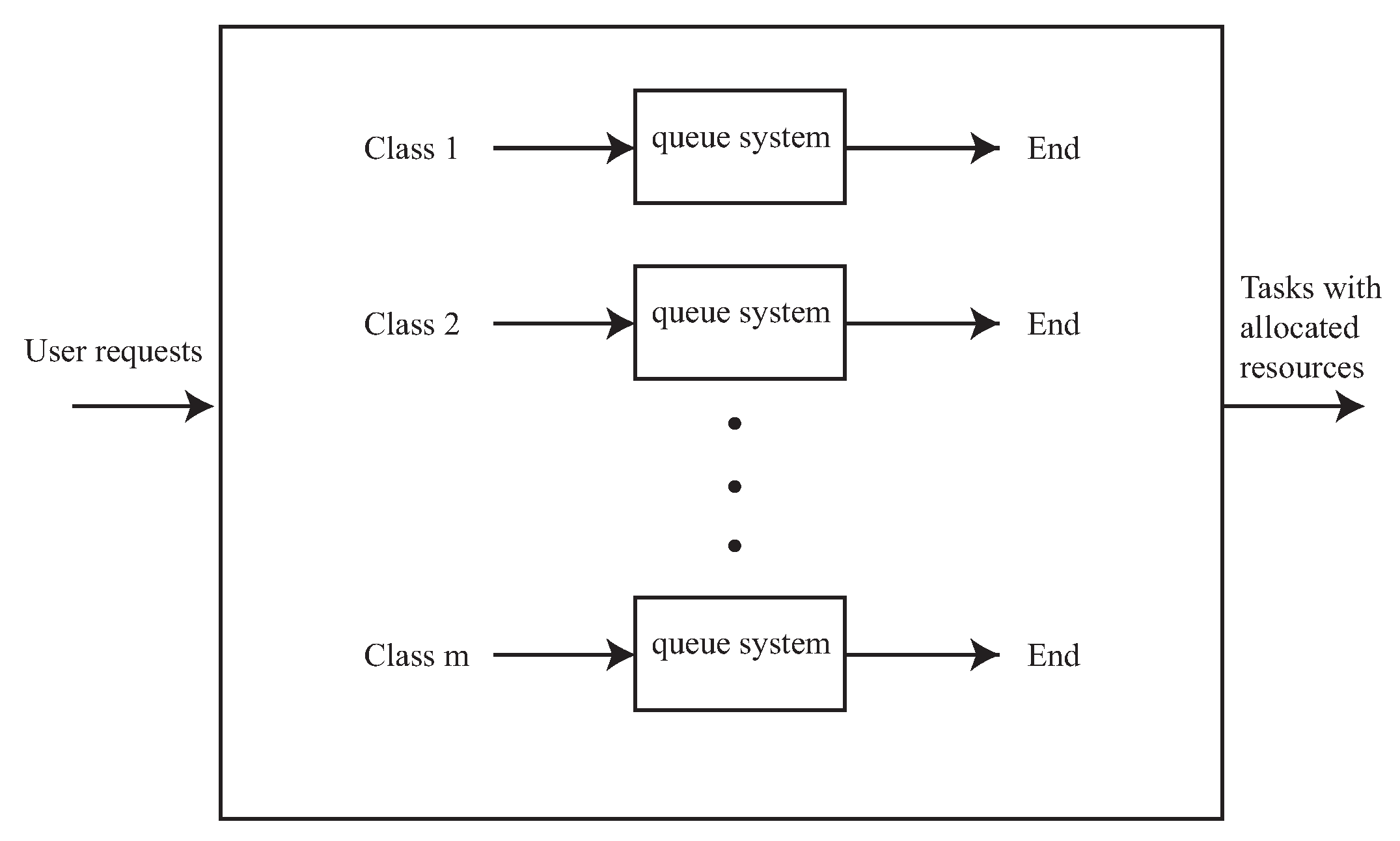
Our resource allocation scheme separates the user demands into classes, based on the dominant resource. Thus, there are m classes. The resource allocator is a central system that handles a set of queue systems. Generally, the resource allocator has 
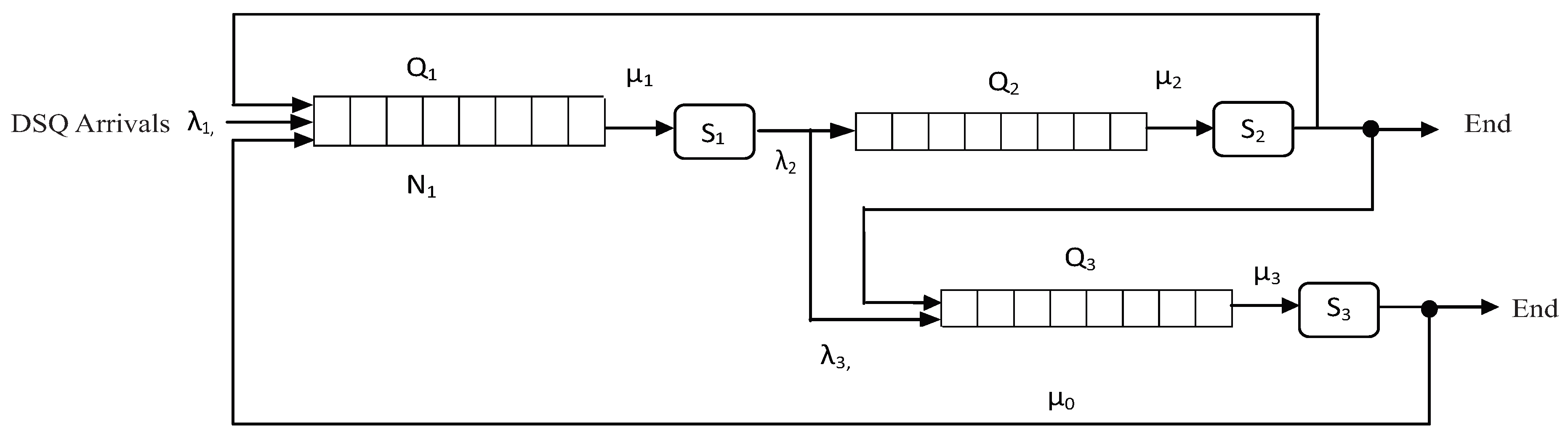
m queue systems, with a structure similar to the one shown in Figure 1, one for each dominant resource. For m = 3 , Figure 1 shows the structure of each queue system exactly. Figure 2 shows the general structure of the resource allocator.
Obviously, inside each queue system j , j [ 1 , , m ] , there are m queues in total, where Q j 1 (queue system j, queue 1) is the DSQ for class j and Q j 2 Q j m are the non-dominant queues. We define the threshold values Φ j , j [ 1 , , m ] as the maximum amounts of dominant resources that will be allocated to users in each queue system of the allocator. For example, Φ 1 shows the maximum amount of resource 1 (dominant resource in queue system 1) that will be allocated, Φ 2 shows the maximum amount of resource 2 (dominant resource in queue system 2) that will be allocated, and so on. These values are necessary, because a resource which is dominant for some users is also requested as non-dominant by other users, so some amount should be saved for this purpose. This amount is expressed by Φ j = T j Φ j and can be incremented, if any dominant amounts are left unallocated. An intuitive way to define the Φ values is to consider them as percentages of the total amounts of the resources available, based on the users’ requests; in other words, they can be expressed as T j × b j , where the b j s are the percentages of available resources per queue, as described in the flow control mechanism.

4.1. An Illustrative Example

To show how our policy can be applied, consider a cloud with three resources available, (CPU, Memory and Disk) = (40, 80 and 50). The mean service rate in all queues is μ = 20 jobs per time unit. The amounts are given in units; a memory and disk unit can have a certain size. There are nine users that compete for these resources and their demands are given in Table 2.
Obviously, the jobs to be generated will either be CPU-intensive or memory-intensive. This means that our allocator will use two of the three available queue systems, 1 and 2. Each of the two systems will have three queues, Q 11 , , Q 13 and Q 21 , , Q 23 , where Q 11 and Q 21 are the DSQs of the two systems. In the first system, Q 11 will accommodate the CPU-intensive jobs, while in the second system, Q 21 will accommodate the memory-intensive jobs.
Algorithm 1 starts with the threshold values Φ 1 and Φ 2 . As discussed in the beginning of this section, an intuitive idea to define Φ 1 would be to find the percentage of CPUs requested as dominant from the total number of requested CPUs. In this example, 37 CPUs are requested as dominant resources (users 1–5) and another 16 as non-dominant resources. In total, 53 CPUs are required; thus, 37/53 = 70 % of the CPU requests are for dominant resources. Thus, Φ 1 = 0.7 × 40 = 28 and Φ 1 = 40 28 = 12 . Similarly, 93 out of the 115 in total memory requests are for dominant resources. This is 81 % , so Φ 2 = 0.81 × 80 = 65 , so Φ 2 = 80 65 = 15 .
Algorithm 1: Describes the resource allocation policy.
1. Find the threshold values Φ j , j [ 1 , , m ] ;
2. Compute Φ j = T j Φ j ; // Non-dominant resources.
3. For all DSQ’s in parallel do
4. Implement the fair policy; // (Steps 1–3; see Section 2.1).
5. Compute i = 1 n F i ; // The total amount of dominant resources
           // allocated.
6.  Φ j = Φ j + Φ j i = 1 n F i ; // Amounts of dominant resources
               // left unallocated.
7. End For;
8. For all non-DSQ’s in parallel do
9. Implement the fair policy using Φ j , the resources
   not allocated as dominant;
10. End For;
The two queue systems execute in parallel, implementing the three steps of our fair policy described in Paragraph II.A. We get V = [ 4 , 6 , 8 , 9 , 10 ] . From Equation (4), we get the maximum number of jobs for each user, U 1 max = 28 4 = 7 , U 2 max = 28 6 = 4.67 , U 3 max = 28 8 = 3.5 , U 4 max = 28 9 = 3.11 , and U 5 max = 28 10 = 2.8 and N = i = 1 n U i max = 7 + 4.67 + 3.5 + 3.11 + 2.8 = 21.08 jobs. From Equation (5), the fair allocations for each job f = T r ^ N = Φ N (as the available resources for the dominant resource, CPU) are Φ 1 = 28/21.08 = 1.33. Thus,
F 1 = 1.33 × U 5 max = 3.72 , F 2 = 1.33 × U 4 max = 4.13 , F 3 = 1.33 × U 3 max = 4.65 , F 4 = 1.33 × U 2 max = 6.20 , F 5 = 1.33 × U 1 max = 9.30 .
Thus, U 1 will get four CPUs, U 2 will get four CPUs, U 3 will get five CPUs, U 4 will get six CPUs and U 5 will get nine CPUs. The total amount of resources allocated is 28 CPUs (step 5 of Algorithm 1); thus, no more resources are added to Φ (Step 6). The dominant server’s utilization p 11 (queue system 1, queue 1) can be found from Equation (7), and it is 95.47 % . Thus the maximum rate at which the jobs are generated in Q 11 for CPU-intensive jobs is λ 11 = 19 jobs per time unit. Similarly, we repeat steps 3 to 6 of Algorithm 1, and find that the second queue system will allocate 12 memory units to U 6 , 15 memory units to U 7 , 17 memory units to U 8 and 20 memory units to U 9 . In total, 64 memory units will be allocated to user jobs having the memory as the dominant resource; thus, from step 6 of the algorithm, we add one more unit to Φ 2 . That is, one more memory unit will be available for jobs whose dominant resource is not the memory. Thus, Φ 2 = 16 . The parameters computed for the second queue system are shown in Table 3. The dominant server’s utilization p 21 (queue system 2, queue 1) can be found from Equation (7), and it is 92 % . Thus, the maximum rate at which the jobs are generated in Q 21 for memory-intensive jobs is λ 21 = 18.4 jobs per time unit.
Returning to the first queue system, it has to allocate memory and disk units to the users with CPUs as their dominant resource demanded. To allocate memory units, it needs to read the value of Φ 2 = 16 (the number of memory units not allocated as dominant resources in the second queue system). These 16 units will be allocated using our fair allocation policy (lines 8 and 9 of Algorithm 1). Table 4 shows the computed values. The jobs will be generated in Q 12 of the first queue system. The server’s utilization p 12 (queue system 1, queue 2) can be found from Equation (7), and it is 96 % . Thus, the maximum rate at which the jobs are generated in Q 12 to allocate memory for CPU-intensive jobs is λ 12 = 19.7 jobs per time unit.
Returning to the second queue system, it has to allocate CPU and disk units to the users with memory as the dominant resource demanded. To allocate CPU units, the value of Φ 1 = 12 needs to be read (the amount of CPU units not allocated as dominant resources in the first queue system). These 12 units will be allocated again using our fair allocation policy. Table 5 shows the computed values. The jobs will be generated in Q 22 of the second queue system. The server’s utilization p 22 (queue system 2, queue 2) can be found from Equation (7), and it is 96 % . Thus, the maximum rate at which the jobs are generated in Q 22 to allocate memory for CPU-intensive jobs is λ 22 = 19.7 jobs per time unit. Allocations in queues Q 12 and Q 22 are also performed in parallel.
Finally, the two systems have to allocate disks to all users. The disk is not the dominant resource for any of the users. Disk allocation will be performed separately based on our fair policy. In total, 68 disk units have been requested by all users: 28 ( 41 % ) from users whose dominant resource was the CPU and 40 ( 59 % ) from users whose dominant resource was the memory. Intuitively, the Φ 3 values are 20 disk units for the first queue system and 30 for the second. As a result, users 1–5 get 1,4,4,5 and 6 disks respectively, from the first system and the system utilization is 0.957%. The maximum rate at which the jobs are generated in Q 31 for the CPU-intensive jobs to which the disks are allocated is 19.15 jobs. Finally, users 6–9 get 6,7,7 and 9 disks respectively from the second system, and the system utilization is 0.925%. The maximum rate at which the jobs are generated in Q 32 for the memory-intensive jobs to which the disks are allocated is 19.5 jobs.

4.2. The Complexity of Our Scheduling Policy

To compute the complexity of the proposed scheduling policy, we have to consider that each queue system has m queues and there are at most m queue systems executing for a resource allocation problem. This gives m 2 queues in total, but since the queue systems can efficiently be executed in parallel (specifically m queues are executed in parallel), the time required to complete the scheduling is O ( m N m a x ) , where N m a x is the maximum number of jobs generated during the allocation process. The solution to Equation (7) also depends on m. Since m is generally limited compared to the number of jobs that can be generated, our scheduling policy can be implemented in O ( N ) time; that is, linear to the number of jobs generated.

5. Experimental Results

This section provides details about our simulation configuration and our results. For our simulation environment, we used an Intel Core i7-8559U Processor system, with clock speed at 2.7 GHz, equipped with four cores and eight threads/core, for a total of 32 logical processors. In our simulations, each user was entitled of up to four CPUs, 4 GB RAM and 40 GB of system disk. We also set one CPU as one CPU unit, 1 GB RAM as one memory unit and 10 GB disk as one disk unit. Thus, the demand (two CPUs, 1 GB RAM and 10 GB disk) would be translated into (2,1,1) and it is CPU-intensive. The demand (one CPU, 3 GB RAM and 20 GB disk) is translated into (1,3,2) and it is memory-intensive. Another idea would be to randomly characterize the jobs, but we preferred the way just described. In our experimental results, we studied the effects of the job generation control rate and the system utilization.

5.1. The Effect of Job Generation Rate Control

To study the effect of job generation rate, we worked as follows:
  • We generated a random number of users, from 50 to 1000, and a set of requests for each user. Additionally, we set different values for the total amount of each available resource, so that, in some cases, the resources available were enough to satisfy all user requests, while in other cases, they were not.
  • We set the maximum value of μ equal to 30 jobs per second; thus, the system’s rate of job generation in the queue systems could not be more than λ = 30 jobs per second.
  • We kept tracking the system’s state at regular time intervals h and recorded the percentages of resources consumed between consecutive time intervals; thus, we computed the b i values. Every time a job i leaves a queue, the system’s state changes. For example, if a job leaves the DSQ, it means that it has consumed F units of the dominant resource, changing the system’s state from K = K 1 , K 2 , K m to K = K 1 F , K 2 , K m . On the other hand, job generation and entrance in the queues over a period of time means that the system’s job generation rate may change.
After running sets of simulations for different user numbers, we averaged the percentages of resources consumed during all the recorded time intervals, for different recorded values of λ i . The results showed that, when the value of λ i increased up to the thresholds defined by Equation (7), the percentage of resources consumed during this interval increased, due to increased utilization. The results are shown in Figure 3. When the number of users is relatively small, an average value of λ i = 15 was enough to consume almost 100% of the resources during this period. For larger number of users (up to 1000), an average job generation rate of up to λ i = 28 (among all queues) was necessary to exhaust the resources requested over the time intervals.

5.2. Resource Utilization

In the second set of experiments, we studied the utilization of each resource independently. The requests were generated in such a manner that the CPU was dominant for 50% of the cases, the memory was dominant for 30% of the cases and the disk was dominant in 20% of the cases. The number of users ranged between 500 and 1000, so that they could exhaust all the resources available. In all the simulation sets, the duration period was one hour, 3600 s. As the time proceeded and resources were being consumed, fewer jobs were generated and the overall resource utilization decreased, but it never dropped below 90%. As can be seen in Figure 4, the CPU utilization began dropping after about 160 s, while the utilization of memory and disk seemed to be dropping in a smoother way and at later times (200 and 240 s, respectively). The peaks seen in this graph represent the cases where some more resources became available and returned to the pool, either due to the scheduling policy or due to returns from finished jobs that returned the resources back to the pool.
In our last set of experiments, we averaged the utilization of all (see Figure 5) the resources under our policy using a small number of users (up to 20), to fairly compare the utilization provided by our policy to the utilization provided by a new algorithm, DRBF [20] (the authors present simulation results for a set of six users). From the results, we see that our policy outperforms the DRBF strategy and achieves utilization of about 98%–99%, while the changes are very small (notice that the line is rather smooth). The DRBF policy achieves a utilization of about 94%–98%, with some peaks where the utilization drops off in a non-smooth fashion. Additionally, note that our strategy was found to achieve a utilization of over 90%, even for a large number of users.

6. Conclusions and Future Work

In this short paper, we present a fair resource allocation policy for cloud computing, which includes a job generation (or flow) control to determine the maximum number of affordable user-tasks at a given time period. The performance analysis showed that the flow control can help to improve the resource utilization. The resource allocator is a central system composed of a total of m 2 queues, for m different resources in the cloud. Because the proposed allocation policy can easily be organized in such a way that batches of m queues can execute in parallel, the complexity of the allocation policy is linear.
In the future, we plan to expand our policy, so that it addresses other important issues, such as the cost of each resource allocated and the execution time. One idea to work on in order to reduce the total execution time, is to pipeline the computations, but careful design is required to avoid delays between the pipeline stages. An interesting research topic would be to try to combine our work with an adaptive monitoring estimation model, such as [6], to include auto-scaling support in our work. That may help with resolving real-life phenomena, such as ping-pong effects or spikes. Since this model includes probabilistic weighting factors, possible incorporation into our model could be examined. Finally, we need to obtain comparable results from other works (including flow control schemes) and compare the total execution time of our policy to the total execution times of other published policies.

Author Contributions

S.S.: Algorithm Scheduling, Mathematical Modeling; S.K.: Implementation and Simulation Results.

Funding

This research received no external funding.

Acknowledgments

This work was partially supported by the project “Algorithms and Applications in Social Networks and Big Data Systems,” which is funded by the Unified Insurance Fund of Independently Employed (ETAA), in Greece.

Conflicts of Interest

The authors declare no conflict of interest.

References

  1. Jennings, B.; Stadler, R. Resource management in clouds: Survey and research challenges. J. Netw. Syst. Manag. 2015, 2, 567–619. [Google Scholar] [CrossRef]
  2. Lu, Z.; Takashige, S.; Sugita, Y.; Morimura, T.; Kudo, Y. An analysis and comparison of cloud data center energy-efficient resource management technology. Int. J. Serv. Comput. 2014, 23, 32–51. [Google Scholar] [CrossRef]
  3. Tantalaki, N.; Souravlas, S.; Roumeliotis, M. A review on big data real-time stream processing and its scheduling techniques. Int. J. Parallel Emerg. Distrib. Syst. 2019. [Google Scholar] [CrossRef]
  4. Tantalaki, N.; Souravlas, S.; Roumeliotis, M.; Katsavounis, S. Linear Scheduling of Big Data Streams on Multiprocessor Sets in the Cloud. In Proceedings of the EEE/WIC/ACM International Conference on Web Intelligence, Thessaloniki, Greece, 14–17 October 2019; pp. 107–115. [Google Scholar]
  5. Xiao, Z.; Song, W.J.; Chen, Q. Dynamic resource allocation using virtual machines for cloud computing environment. IEEE Trans. Parallel Distrib. Syst. 2013, 24, 1107–1117. [Google Scholar] [CrossRef]
  6. Trihinas, D.; Georgiou, Z.; Pallis, G.; Dikaiakos, M.D. Improving Rule-Based Elasticity Control by Adapting the Sensitivity of the Auto-Scaling Decision Timeframe. In Proceedings of the Third International Conference on Algorithmic Aspects of Cloud Computing (ALGOCLOUD 2017), Vienna, Austria, 5 September 2017. [Google Scholar]
  7. Copil, G.; Trihinas, D.; Truong, H.; Moldovan, D.; Pallis, G.; Dustdar, S.; Dikaiakos, M.D. ADVISE—A Framework for Evaluating Cloud Service Elasticity Behavior. In Proceedings of the 12th International Conference on Service Oriented Computing (ICSOC 2014), Paris, France, 3–6 November 2014. [Google Scholar]
  8. Ghodsi, A.; Zaharia, M.; Hindman, B.; Konwinski, A.; Shenker, S.; Stoica, I. Dominant resource fairness: Fair allocation of multiple resource types. In Proceedings of the 8th USENIX conference on Networked systems design and implementation, Boston, MA, USA, 30 March–1 April 2011; pp. 323–336. [Google Scholar]
  9. Souravlas, S.; Sifaleras, A.; Katsavounis, S. A Parallel Algorithm for Community Detection in Social Networks, Based on Path Analysis and Threaded Binary Trees. IEEE Access 2019, 7, 20499–20519. [Google Scholar] [CrossRef]
  10. Souravlas, S.; Sifaleras, A.; Katsavounis, S. A novel, interdisciplinary, approach for community detection based on remote file requests. IEEE Access 2018, 6, 68415–68428. [Google Scholar] [CrossRef]
  11. Souravlas, S.; Sifaleras, A. Binary-Tree Based Estimation of File Requests for Efficient Data Replication. IEEE Trans. Parallel Distrib. Syst. 2017, 28, 1839–1852. [Google Scholar] [CrossRef]
  12. Bodrul Alam, A.B.M.; Zulkernine, M.; Haque, A. A reliability-based resource allocation approach for cloud computing. In Proceedings of the 2017 7th IEEE International Symposium on Cloud and Service Computing, Kanazawa, Japan, 22–25 November 2017; pp. 249–252. [Google Scholar]
  13. Kumar, N.; Saxena, S. A preference-based resource allocation in cloud computing systems. In Proceedings of the 3rd International Conference on Recent Trends in Computing 2015 (ICRTC-2015), Delhi, India, 12–13 March 2015; pp. 104–111. [Google Scholar]
  14. Lin, W.; Wang, J.Z.; Liang, C.; Qi, D. A threshold-based dynamic resource allocation scheme for cloud computing. Procedia Eng. 2011, 23, 695–703. [Google Scholar] [CrossRef]
  15. Tran, T.T.; Padmanabhan, M.; Zhang, P.Y.; Li, H.; Down, D.G.; Christopher Beck, J. Multi-stage resource-aware scheduling for data centers with heterogeneous servers. J. Sched. 2018, 21, 251–267. [Google Scholar] [CrossRef]
  16. Hu, Y.; Wong, J.; Iszlai, G.; Litoiu, M. Resource provisioning for cloud computing. In Proceedings of the 2009 Conference of the Center for Advanced Studies on Collaborative Research, Toronto, ON, Canada, 2–5 November 2009; pp. 101–111. [Google Scholar]
  17. Khanna, A.; Sarishma. RAS: A novel approach for dynamic resource allocation. In Proceedings of the 1st International Conference on Next Generation Computing Technologies (NGCT-2015), Dehradun, India, 4–5 September 2015; pp. 25–29. [Google Scholar]
  18. Saraswathia, A.T.; Kalaashrib, Y.R.A.; Padmavathi, S. Dynamic resource allocation scheme in cloud computing. Procedia Comput. Sci. 2015, 47, 30–36. [Google Scholar] [CrossRef]
  19. Souravlas, S. ProMo: A Probabilistic Model for Dynamic Load-Balanced Scheduling of Data Flows in Cloud Systems. Electronics 2019, 8, 990. [Google Scholar] [CrossRef]
  20. Zhao, L.; Du, M.; Chen, L. A new multi-resource allocation mechanism: A tradeoff between fairness and efficiency in cloud computing. China Commun. 2018, 24, 57–77. [Google Scholar] [CrossRef]
Figure 1. Resource allocation model with three resources; i = 1 is the dominant resource.
Electronics 08 01348 g001
Figure 2. Resource allocator with m queue systems.
Electronics 08 01348 g002
Figure 3. The effect of the job generation rate.
Electronics 08 01348 g003
Figure 4. Individual resource utilization over a period of one hour.
Electronics 08 01348 g004
Figure 5. Average resource utilization with a small number of users (up to 20).
Electronics 08 01348 g005
Table 1. Summary of related papers, based on the metrics used to evaluate resource allocation (RA).
Resource Allocation SchemeCostExecution TimeUtilization
RA as optimization problem, Alam et al., [12]YesNoNo
Open market-driven auction/preference-driven payment process, Kumar et al. [13]YesNoYes
Threshold-based strategy for monitoring and predicting the users’ demands, Lin et al. [14]YesYesNo
Job class-based strategy, Hu et al. [16]YesNoNo
Dynamic RAS (Resource Allocation System), Khanna et al. [17]NoNoYes
3-stage mapping scheme, Tran et al. [15]YesYesNo
Job feature-based strategy, Saraswathia et al. [18]NoNoYes
Skewness minimization, Xiao et al. [5]NoNoYes
Our workNoNoYes
Table 2. Data for our illustrative example.
UserCPUMemoryDisk
1432CPU-intensive
2645
3856
4967
51028
631810Memory-intensive
73218
852410
953012
Table 3. Computed values for memory (dominant resource) allocation by the second queue system of our example.
Demand Vector (Sorted)Max. No of Jobs/UserFair Allocation/Job, fAllocation Per User, F i
18 U 6 max = 65 / 18 = 3.61 5.6112
21 U 7 max = 65 / 21 = 3.10 15
24 U 8 max = 65 / 24 = 2.71 17
30 U 9 max = 65 / 30 = 2.17 20
Table 4. Computed values for memory (non dominant resource) allocation by the first queue system of our example.
Demand Vector (Sorted)Max. No of Jobs/UserFair Allocation/Job, fAllocation Per User, F i
2 U 1 max = 16 / 2 = 8 0.692
3 U 2 max = 16 / 3 = 5.33 2
4 U 3 max = 16 / 4 = 4 3
5 U 4 max = 16 / 5 = 3.20 4
6 U 4 max = 16 / 6 = 2.67 5
Table 5. Computed values for CPU (non dominant resource) allocation by the second queue system of our example.
Demand Vector (Sorted)Max. No of Jobs/UserFair Allocation/Job, fAllocation Per User, F i
3 U 6 max = 12 / 3 = 4 0.692
3 U 7 max = 12 / 3 = 4 2
5 U 8 max = 12 / 5 = 2.4 3
5 U 9 max = 12 / 5 = 2.4 3

