Model-Based Latency Compensation for Network Controlled Modular Multilevel Converters

Abstract

The use of an internal digital communication network enhances the scalability, implementation and maintenance of Modular Multilevel Converters (MMC). However, it also introduces delays that limit the sampling frequency and the controller dynamic performance. In this paper, we propose a model-based predictor to compensate for the loop delay and overcome these limitations. Two benefits of this approach are possible: either designers can increase the sampling rate and control performance or employ a slower communication protocol/technology. In this paper, we present the mathematical description of the model-based predictor, assess the parameter sensitivity, and show matching simulation and experimental results that validate it. As constraints introduced by the use of digital communications are overcome, the results achieved encourage engineers to adopt a network into the design of Modular Multilevel Converters.

1. Introduction

Modular Multilevel Converters (MMCs) are built by series connections of identical modules (or cells). The number of cells in a converter depends on the nominal terminal voltage and the reliability requirements, with industrial MMCs reported in the literature in the medium, high, and extra high voltage levels [1,2]. As the typical cell blocking voltage is between 1.7 kV (IGBTs) and 6.5 kV (IGCTs or IGBTs) [3], the possible number of cells per arm can go from just a few to hundreds.

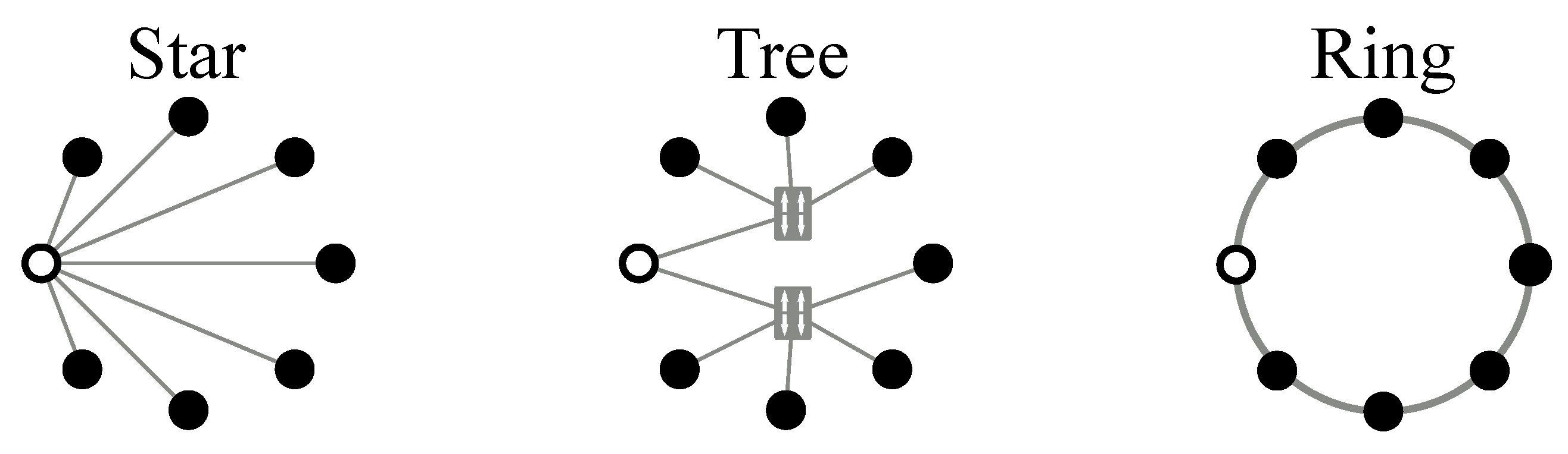
The wide range in the number of cells is a challenge for the control hardware. Moreover, as the converter voltage ratings increase, the control architecture termed star (Figure 1), i.e., single connections between the central controller and the cells leads to an overwhelming amount of interfaces, cables and/or fiber optics that quickly become impracticable in industrial converters or at least unreliable and cumbersome to assemble.

Several authors studied the use of a digital communication network in this context with the purpose of improving the scalability, implementation, and maintenance of such converters. Toh and Norum compared the Ethernet-based protocols EtherCAT, Profinet IRT, and PESNet. They found that the first has the best performance [4], together with low synchronization error/jitter [5,6] and fault tolerance [7]. Carstensen et al. [8] developed the protocol SyCCo bus specifically for modular converters that uses EtherCATsummation frame and on-the-fly processing. Tu and Lukic [9] compared an improved implementation of this protocol with PESNet and found it to allow 28% higher switching frequency in a 30-cell converter. Hillers, Tu and Biela [10] discussed the implications of the control structure for the system reliability when using a communication network. Researchers from Aalborg University implemented a partly distributed control in an MMC prototype to reduce the data shared globally and demonstrated single fault tolerance when using EtherCAT [11,12,13,14]. Reducing the amount of data sent through the communication link has also been the core idea in [15,16].

The choice of a network solution in this application domain needs to consider multiple aspects (see [17]), but, from the review above, we notice that reliability and performance are key factors. All the works listed addressed the former by adopting a ring topology (Figure 1) because it is the simplest one to offer two disjoint paths between any two nodes. When it comes to performance, they used two non-exclusive strategies: to employ high bandwidth links with short forwarding delays and to reduce the communication payload. Corrêa and Almeida [18] explored both strategies and shortened the Minimum Cycle Time (MCT), the time necessary to update all the cells with new information, by a factor of 2.5 compared with EtherCAT in a ring network with 400 nodes.

This work approaches the performance issue from a different side. A model-based predictor compensates for the latency of the network, so the control tolerates longer delays, achieving higher flexibility in the choice of the protocol and communication technology. An alternative benefit is a better dynamic performance because of a higher sampling rate and controller gains.

The use of a plant model to compensate for the loop delay dates back to 1957 when O.J. Smith proposed what today is known as the Smith predictor [19]. Recently, Cortes et al. adopted a similar approach to compensate for the delay introduced by Model Predictive Control calculations [20,21]. The main contributions of this work are: adoption of a model-based predictor for compensating the additional latency introduced by the communication network; description of modulation and balancing schemes pertinent to network controlled MMCs and its relation to the proposed estimation algorithm; assessment of parameter variations in the control performance; and validation of the concept in an experimental set-up.

This paper is organized as follows: first, Section 2 explains how the network introduces a loop delay and how this delay relates with the controller sampling rate. Then, Section 3 presents a model of the Modular Multilevel Converter, discusses the influence of loop delay and sampling periods in the closed-loop control, and shows how the network delay influences the sorting algorithm for capacitor voltage balancing. Next, Section 4 describes the proposed method in mathematical terms, and Section 5 investigates the effect of parameter variations in the closed-loop response. Finally, Section 6 validates the proposed method through Matlab/Simulink simulations and experimental results.

2. Network Induced Latency

The control structure of Modular Multilevel Converters consists of a central unit and embedded electronics in each cell or group of cells. The central controller has powerful computational resources and more access to data than the cells, e.g., measurements and setpoints from higher hierarchy levels, hence it calculates the load current and outer control loops. Its output can be on/off commands, individual references, or a single setpoint per arm [14]. Until Section 4.2, we will be concerned with the flow of information from the central controller to the cells. In addition, On/Off commands will be ignored in this work because the Ethernet-based communications considered fail to provide the sub-microsecond latency necessary to keep the error in the generated voltage small.

The adoption of a real-time protocol translates into a deterministic delay and Minimum Cycle Time (MCT). When the controller outputs individual references to the cells or a single one per arm, the MCT defines the minimum possible actuation delay because the cells must simultaneously apply the new references to avoid a variable loop delay.

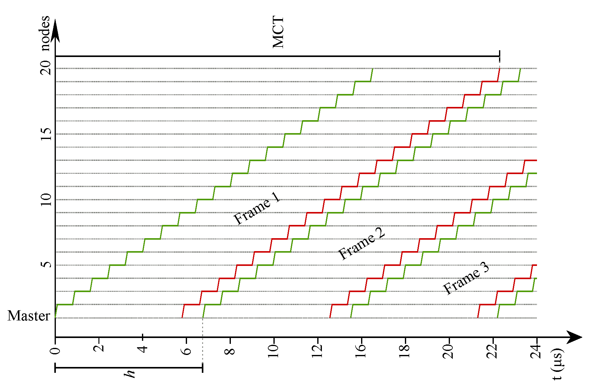
Often, authors take the MCT, the sampling-to-actuation delay, and the control sampling frequency as the same variable, but it must not be so. Consider Ethernet frames traveling around a network when the master node sends a new packet just after the interframe gap has elapsed (Figure 2). Due to the propagation and forwarding delays, i.e., how long a node takes to receive and resend a packet to the next one, the MCT is higher than the time between the arrival of two consecutive packets in a node, i.e., the sampling period h.

The Minimum Cycle Time of EtherCAT, an industrial protocol that has gained popularity in this application domain [22], is expressed by (1) [23],

$$\begin{array}{cc}\hfill MCT& =P.T_{\mathrm{byte}}+⌈\frac{P}{1488}⌉·50·T_{\mathrm{byte}}+\kappa ·T_{\mathrm{fw}},\hfill \end{array}$$

(1)

where P is the data payload in bytes, $⌈x⌉$ is the ceiling of x, $T_{\mathrm{byte}}$ is the time to transmit one byte, $T_{\mathrm{fw}}$ is the forwarding delay (typically between 0.7 µs and 1 µs [24]), and $\kappa$ is the number of nodes. In (1), the first term corresponds to the time to transmit the payload; the second term to the overhead due to packet headers, interframe gap, and frame check sequence; the third to the sum of the nodes forwarding delay. This last term does not influence the sampling period.

As EtherCAT supports only a bit rate of 100 Mbps ($T_{\mathrm{byte}}$= 80 ns), the MCT of a frame with minimum payload is equal to 10.2 µs, 13.7 µs, 41.7 µs or 76.7 µs for a network with 5, 10, 50 or 100 nodes, respectively. However, independently of the network size and the forwarding delay (see Figure 2), the minimum sampling period is 6.7 µs, as it depends only on the smallest Ethernet frame length and the interframe gap that are 72 and 12 bytes long, respectively [25].

In practice, a chain of tasks prevents the controller of reaching such low sampling periods. For example, the central unit has to convert the analog signals and calculate the outputs of the control algorithms; the protocol stack has to prepare the data and handle them to the Medium Access Controller (MAC); then, the MAC has to command the physical layer to send the packet. In our experimental set-up, for example, measurement conversion and control calculations take 27 µs. An optimized EtherCAT master stack can transmit small frames (~72 bytes long) within 11 µs [26], hence, in this particular case, the minimum sampling period would be 38 µs, unless the controller can pipeline some of these tasks.

It is also important to consider the discrete nature of the controller since it causes a range of sampling periods to represent the same amount of delay. The loop delay n, in number of samples, is

$$\begin{array}{cc}\hfill n& =⌈\frac{\varsigma }{h}⌉,\hfill \end{array}$$

(2)

where $\varsigma$ is the sampling-to-actuation delay and h is the sampling period.

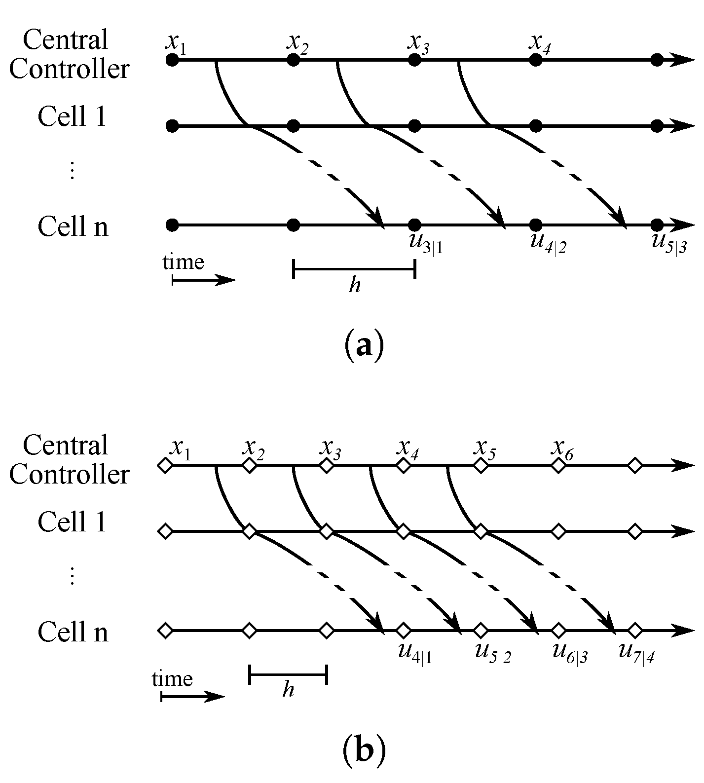
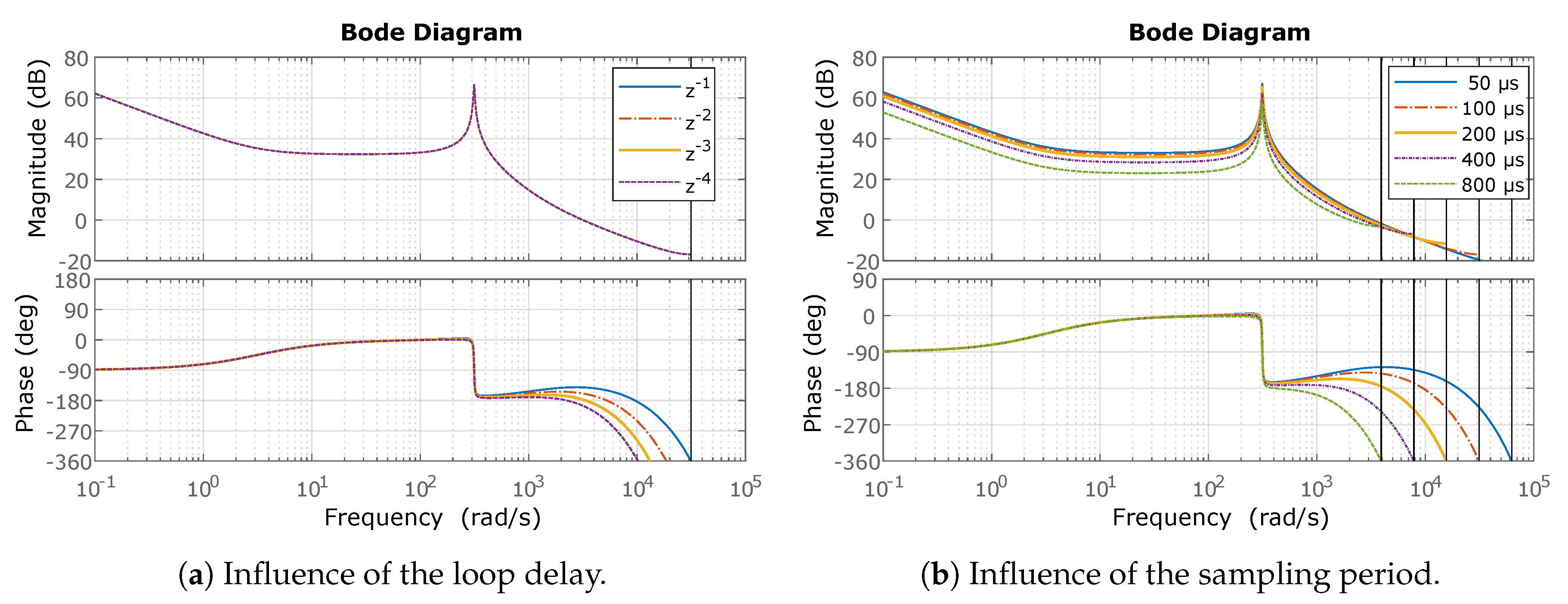
As an illustration, the diagram of Figure 3 shows a network with the control running at two different rates. In the first case (a), the network introduces a delay of one sample, but, in the second case (b), it introduces a delay of two samples due to the shorter sampling period. In an implementation that has a sampling-to-actuation delay just below 100 µs, the loop delay is one sample, just like any discrete controlled system, as long as the sampling period is more than 100 µs. The communication latency would represent a delay of one or two samples, if the sampling period is in the range [50 µs, 100 µs) or [33 µs, 50 µs), respectively, and the sampling-to-actuation delay would be two or three samples.

3. Modular Multilevel Converter Model

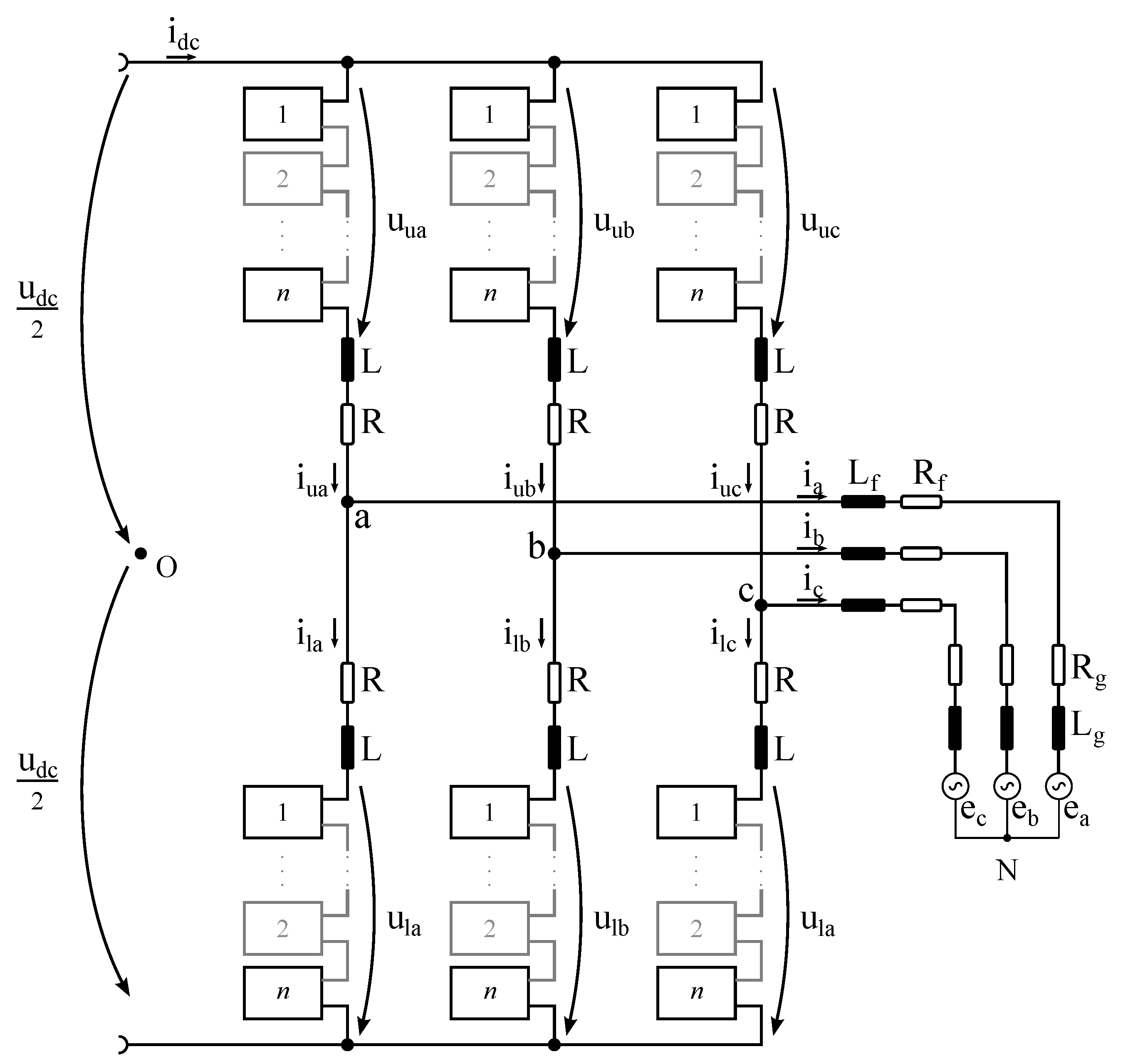
Double-star Modular Multilevel Converters (Figure 4) with half-bridge cells produce AC voltages with $N+1$ or $2N+1$ levels depending on the modulation strategy [27], where N is the number of cells per arm. In the medium voltage range, the converter has a low number of cells, yet their switching frequency is high (~1–2 kHz). As the voltage increases, the cell switching rate approaches the grid frequency, but the number of levels is higher as well as the apparent switching frequency on the load. As a result, in both cases, an inductive output filter is sufficient to fulfill the current and voltage harmonic distortion requirements.

The internal current loops have the fastest dynamics and are the most affected by the loop delay; therefore, we need to model the converter to analyze them. By transforming (3.7) from [28] to the $dq$ reference-frame, we obtain the differential Equations (3) that model the load current dynamics,

$$\begin{array}{cc}\hfill \dot{\left[\begin{array}{c}{i}_d\\ i_q\end{array}\right]}& =\left[\begin{array}{cc}-\frac{R_{eq}}{L_{\mathrm{eq}}}& {\omega }_o\\ -{\omega }_o& -\frac{R_{eq}}{L_{\mathrm{eq}}}\end{array}\right]\left[\begin{array}{c}{i}_d\\ i_q\end{array}\right]+\frac{1}{L_{eq}}\left[\begin{array}{c}{u}_{sd}\\ u_{sq}\end{array}\right]-\frac{\mathbf{1}}{L_{eq}}\left[\begin{array}{c}{e}_d\\ e_q\end{array}\right],\hfill \end{array}$$

(3)

where $e_{dq}$ is the grid voltage, $u_{s,dq}=\left(u_{ldq}-u_{udq}\right)/2$ is the output voltage, $L_{eq}=L/2+L_g+L_f$ is the equivalent inductance, $R_{eq}=R/2+R_g+R_f$ is the equivalent resistance, and ${\omega }_o$ is the grid angular frequency. We list the main parameters of the MMC studied in

Table 1. Simulation and prototype parameters.

Parameter	Value	Parameter	Value
Rated power	50 kVA	Arm inductor (L)	0.5 mH
Grid line voltage	400 V	Arm resistance (R)	1 m$\Omega$
Cells/arm (N)	5	Filter inductor ($L_f$)	5 mH
Cell capacitor (C)	2.2 mF	Filter resistance ($R_f$)	14 m$\Omega$
Sampling period (h)	100 $\mathsf{\mu }$s	Grid inductance	0.4 mH
Carrier frequency	750 Hz	DC voltage	750 V

.

In an MMC, the load current is only one component of the upper and lower arm currents. A second component, known as circulating current, flows through both arms and is defined as $i_{circ,a}\stackrel{\Delta }{=}\left(i_{ua}+i_{la}\right)/2=i_{ua}-i_a/2=i_{la}+i_a/2.$ Their dynamics are necessary for a complete MMC model, as in Equation (4) [28],

$$\begin{array}{cc}\hfill \dot{\left[\begin{array}{c}{i}_{circ,a}\\ i_{circ,b}\\ i_{circ,c}\end{array}\right]}& =\left[\begin{array}{ccc}-\frac{R}{L}& 0& 0\\ 0& -\frac{R}{L}& 0\\ 0& 0& -\frac{R}{L}\end{array}\right]\left[\begin{array}{c}\begin{array}{c}{i}_{circ,a}\\ i_{circ,b}\\ i_{circ,c}\end{array}\end{array}\right]+\frac{1}{L}·\frac{U_{dc}}{2}-\frac{1}{L}\left[\begin{array}{c}{u}_{circ,a}\\ u_{circ,b}\\ u_{circ,c}\end{array}\right],\hfill \end{array}$$

(4)

where the internal voltage is $u_{circ,abc}=\left(u_{l,abc}+u_{u,abc}\right)/2$. The number of inserted cells in the upper and lower arms, know as insertion indexes $n_u$ and $n_l$, are [28]

$$\begin{array}{cc}\hfill \begin{array}{c}{n}_u=\frac{u_{circ}^{*}-u_s^{*}}{u_{cu}^{\Sigma }}\end{array}& n_l=\frac{u_{circ}^{*}+u_s^{*}}{u_{cl}^{\Sigma }},\hfill \end{array}$$

(5)

where $u_{cu}^{\Sigma }$ and $u_{cl}^{\Sigma }$ are the sum of the capacitor voltages of the upper and lower arms, respectively, and the superscript * denotes reference values.

Influence of Sampling Rate and Delay on Control Performance

Sampling is a fundamental property of discrete-controlled systems. Its rate influences the poles and zeros of the discretized plant, hence it affects the controller design and closed-loop response [29]. In like manner, loop delays are a common phenomenon in several control applications and are almost inevitable in networked controlled systems [30]. Their presence imposes strict limitations on achievable feedback performance and often has a “destabilizing effect” [30].

The frequency-domain analysis is the preferred way of dealing with systems that have loop delays [19,29,30]. Consider open-loop Bode diagram (Figure 5), correspondent to the inner current loop of our prototype converter (parameters listed in Table 1) with a Proportional-Integral (PI) controller in synchronous reference frame tuned for 3 ms settling time $t_s$ using the pole placement method. Each delay of one sample introduces a linearly increasing lag with frequency [30] (at the Nyquist frequency, the phase is −360°, −540°, −720° for delays of 1, 2 or 3 samples, respectively), but it does not affect the magnitude (Figure 5a). A discrete-time controller has a delay of at least one sample. With two samples, the system has a narrow phase margin, and with three or more it becomes unstable (negative phase margin).

The Bode diagram of Figure 5b shows the influence of the sampling frequency on the phase margin and crossover frequency when the plant has a single delay. For the case analyzed, the three shortest sampling periods result in positive phase margins of 52°, 39°, and 16°, respectively, i.e., only them result in a stable closed-loop system.

However, the control of the converter is possible with lower sampling frequencies or longer delays, but the designer will need to reduce the controller gains to bring the system back to stability [19] (e.g., in Ziegler–Nichols method, the integral gain is inversely proportional to the deadtime [29]) and, consequently, slow down its response.

4. Proposed Estimation Algorithm

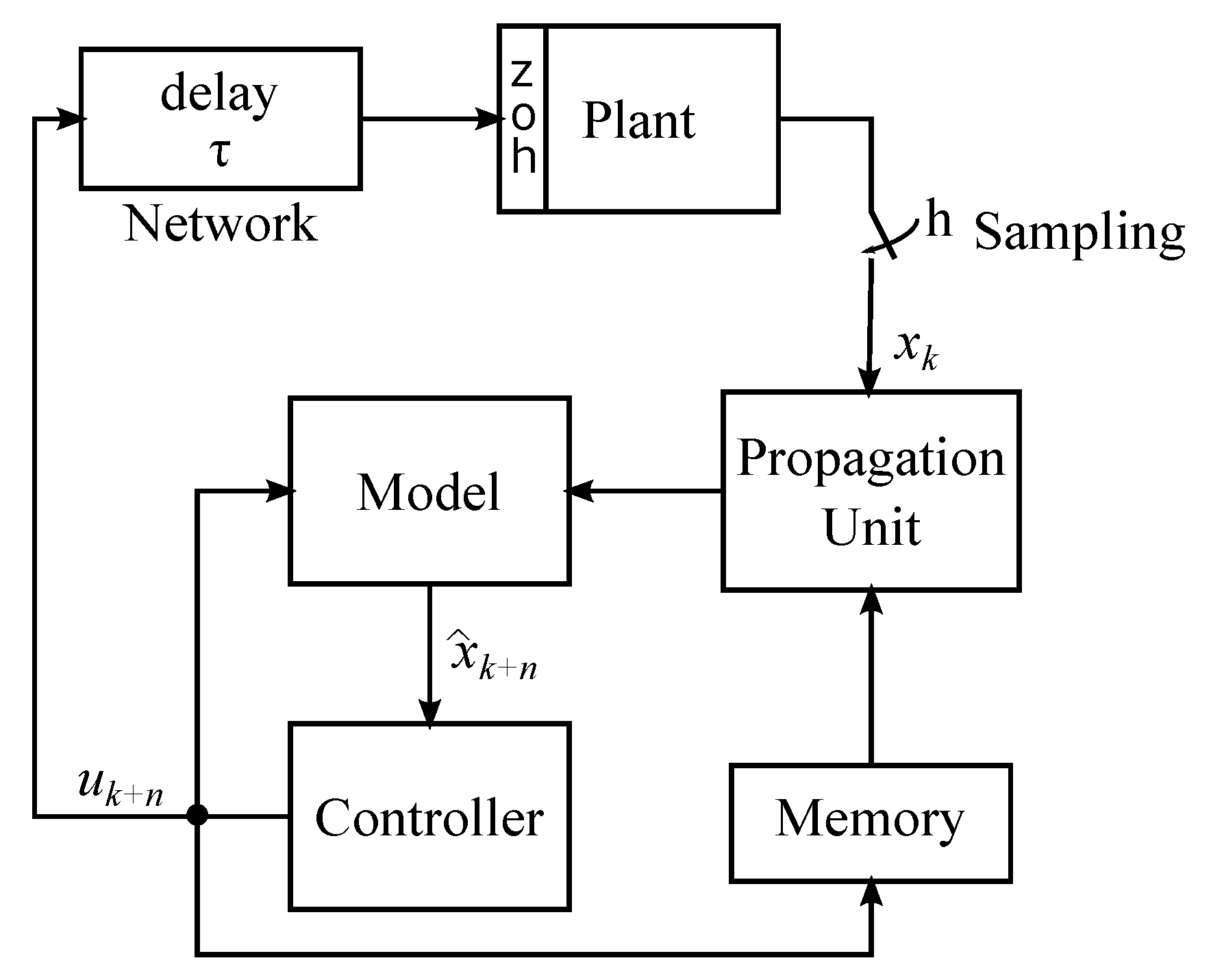
In this section, we explain the model-based predictor and how it compensates for loop delays. It works as follows: a model of the plant predicts what will be the state vector n samples ahead based in the measured state vector and the known future plant inputs. The central unit feeds the estimated states back to the controller that calculates the plant inputs and places them into the communication queue. After n samples, the inputs are applied to the plant (Figure 6).

Consider the difference state-space Equations (6) and (7) that represent a discretized linear time-invariant model,

$$\begin{array}{cc}\hfill {\mathit{x}}_{k+1}& =\mathbf{A}{\mathit{x}}_k+\mathbf{B}{\mathit{u}}_{k|k-n},\hfill \end{array}$$

(6)

$$\begin{array}{cc}\hfill {\mathit{y}}_k& =\mathbf{C}{\mathit{x}}_k,\hfill \end{array}$$

(7)

where ${\mathit{x}}_k$ and ${\mathit{y}}_k$ are the state and output vectors in instant k, respectively, ${\mathit{u}}_{k|k-n}$ is the plant input vector in instant k calculated in $k-n$, and $\mathit{A}$, $\mathit{B}$, and $\mathit{C}$ are matrices of the necessary dimensions.

In a state-feedback control law, the plant input would be ${\mathit{u}}_k=\mathbf{K}{\mathit{x}}_k$, where $\mathbf{K}$ is the gain matrix that can be designed, for example, using Linear Quadratic Gaussian control or pole placement [29]. To compensate for the loop delay, we propose to predict the system state ${\widehat{\mathit{x}}}_{k+n}$ and use it for the calculation of the plant input, as in Equation (8).

$$\begin{array}{cc}\hfill {\mathit{u}}_{k+n|k}& =\mathbf{K}{\widehat{\mathit{x}}}_{k+n}.\hfill \end{array}$$

(8)

Henceforth, we will drop the notation ${\mathit{u}}_{k+n|k}$ and use only ${\mathit{u}}_{k+n}$ because the network has a constant delay, guaranteed by the real-time communication, and the controller always calculates the plant input n samples in advance.

The estimated states $\widehat{\mathit{x}}$ in instants $k+1$ to $k+n$ are

$$\begin{array}{cc}\hfill {\widehat{\mathit{x}}}_{k+1}& =\widehat{\mathbf{A}}{\mathit{x}}_k+\widehat{\mathbf{B}}{\mathit{u}}_k,\hfill \end{array}$$

(9)

$$\begin{array}{cc}\hfill {\widehat{\mathit{x}}}_{k+2}& =\widehat{\mathbf{A}}{\widehat{\mathit{x}}}_{k+1}+\widehat{\mathbf{B}}{\mathit{u}}_{k+1},\hfill \\ & ⋮\hfill \end{array}$$

(10)

$$\begin{array}{cc}\hfill {\widehat{\mathit{x}}}_{k+n}& =\widehat{\mathbf{A}}{\widehat{\mathit{x}}}_{k+n-1}+\widehat{\mathbf{B}}{\mathit{u}}_{k+n-1},\hfill \end{array}$$

(11)

or, in a recursive manner,

$$\begin{array}{cc}\hfill {\widehat{\mathit{x}}}_{k+n}& ={\widehat{\mathbf{A}}}^n{\mathit{x}}_k+\sum _{j=1}^n{\widehat{\mathbf{A}}}^{j-1}\widehat{\mathbf{B}}{\mathit{u}}_{k+n-j},\hfill \end{array}$$

(12)

where matrices $\widehat{\mathbf{A}}$ and $\widehat{\mathbf{B}}$ correspond to the plant model and can be obtained by the digitalization of Equations (3) or (4). If we substitute (12) in (8), the plant input vector is expressed by

$$\begin{array}{cc}\hfill {\mathit{u}}_{k+n}& =\mathbf{K}{\widehat{\mathbf{A}}}^n{\mathit{x}}_k+\sum _{j=1}^n\mathbf{K}{\widehat{\mathbf{A}}}^{j-1}\widehat{\mathbf{B}}{\mathit{u}}_{k+n-j}.\hfill \end{array}$$

(13)

The controller calculates (13) every cycle and puts the results in the communication queue. A new measurement is only necessary to calculate the first term of (13), $\mathbf{K}{\widehat{\mathbf{A}}}^n{\mathit{x}}_k$. All the other terms can be evaluated as soon as the next plant input vector is available, as ${\mathit{u}}_{k+n}\to {\mathit{u}}_{k+n-1}$, ..., ${\mathit{u}}_{k+1}\to {\mathit{u}}_k$ in the next sample. Note that the matrices $\mathbf{K}{\widehat{\mathbf{A}}}^n$, $\mathbf{K}\widehat{\mathbf{B}}$ to $\mathbf{K}{\widehat{\mathbf{A}}}^{n-1}\widehat{\mathbf{B}}$ have constant elements that can be stored in the memory at compilation time, so this method is not hard on the processing system.

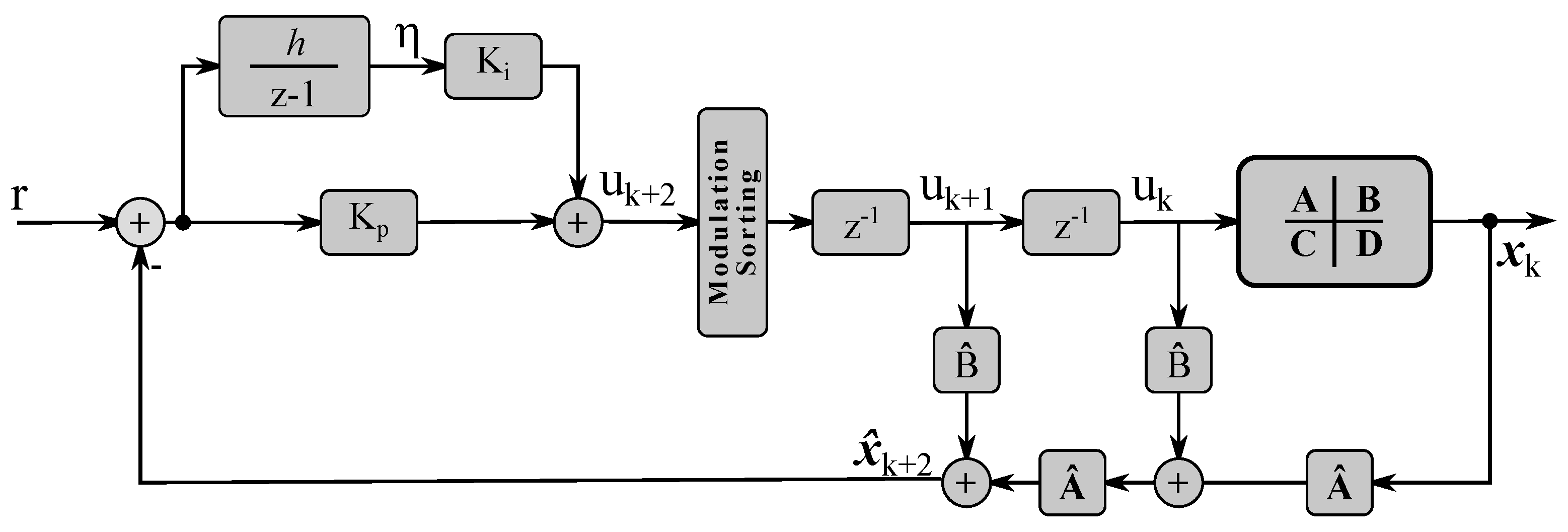
As an illustration, we represented the closed-loop system with two actuation delays, a PI controller, and the model-based predictor in the block diagram of Figure 7 that corresponds to the current control-loop of an MMC. In this system, the augmented state-space vector is ${\left[\begin{array}{cccc}\mathit{x}& {\mathit{u}}_k& {\mathit{u}}_{k+1}& \mathit{\eta }\end{array}\right]}^T$ to include the plant input ${\mathit{u}}_k$, the future plant input ${\mathit{u}}_{k+1}$, and the controller integral part $\mathit{\eta }$. The output of the PI controller will be equal to the plant input two samples ahead (n = 2) and (13) becomes ${\mathit{u}}_{k+2}=\mathbf{K}{\widehat{\mathbf{A}}}^2{\mathit{x}}_k+\mathbf{K}\widehat{\mathbf{B}}{\mathit{u}}_{k+1}+\mathbf{K}\widehat{\mathbf{A}}\widehat{\mathbf{B}}{\mathit{u}}_k$. From the block diagram, it is possible to deduce the state-space closed-loop response (14) in the format of (6):

$$\begin{array}{cc}\hfill {\left[\begin{array}{c}\mathit{x}\\ {\mathit{u}}_k\\ {\mathit{u}}_{k+1}\\ \mathit{\eta }\end{array}\right]}_{k+1}& =\left[\begin{array}{cccc}\mathit{A}& \mathit{B}& \mathbf{0}& \mathbf{0}\\ \mathbf{0}& \mathbf{0}& \mathit{I}& \mathbf{0}\\ -k_p{\widehat{\mathbf{A}}}^2& -k_p\widehat{\mathbf{A}}\widehat{\mathbf{B}}& -k_p\widehat{\mathbf{B}}& k_i\mathit{I}\\ -{\widehat{\mathbf{A}}}^{2}h& -\widehat{\mathbf{A}}\widehat{\mathbf{B}}h& -\widehat{\mathbf{B}}h& \mathit{I}\end{array}\right]·\left[\begin{array}{c}\mathit{x}\\ {\mathit{u}}_k\\ {\mathit{u}}_{k+1}\\ \mathit{\eta }\end{array}\right]+\left[\begin{array}{c}\mathbf{0}\\ 0\\ k_p\mathit{I}\\ \mathit{I}h\end{array}\right]·\mathit{r},\hfill \end{array}$$

(14)

where $\mathit{r}$ is the reference vector, $\mathbf{I}$ is the identity matrix of proper dimensions, h is the sampling period, and $k_p$ and $k_i$ are the proportional and integral gains, respectively.

4.1. Estimation of Circulating Current

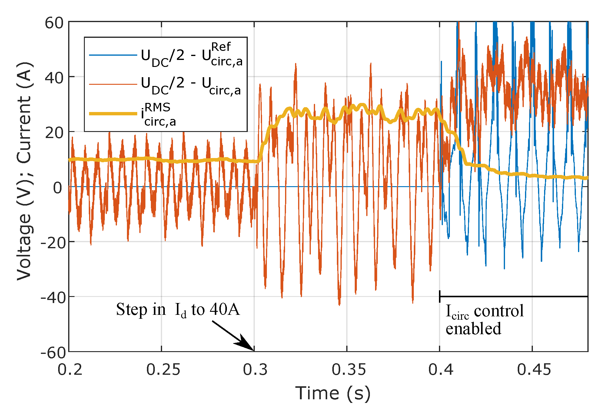
Though (12) is valid for both the load and the circulating current state vectors, the correct estimation of the latter is difficult. The reason is the appearance of parasitic components in the synthesized voltages due to the difference between the divisors of (5) and the effective summed voltage of the inserted capacitors (see subchapter 3.5 of [28]). Because the voltage drop in L and R are small ($u_l+u_u\simeq u_{dc}$), even parasitic components with low magnitude produce significant errors between the reference and the applied internal voltage $u_{circ,abc}^{*}$. In Figure 8, we show a simulation of the $u_{circ,a}$ (orange waveform) and its reference (blue waveform) when the circulating current control is disabled ($t<0.4$ s) and enabled ($t>0.4$ s). In both cases, the difference between reference and measurement is remarkable, though the control is still able to reduce the circulating current RMS value (yellow waveform) when enabled.

Two solutions to this problem are possible. The first one is to use the arm voltage measurements as $u_k$ in (12) to estimate the future circulating current state vector, but, in this case, the prediction is limited to a single sample in the future. The second one is to limit the circulating current with a large arm inductance passively to avoid the need for an active method.

4.2. Modulation and Capacitor Balancing

Thus far, we have only considered the calculation of the voltage references by the load and circulating current controllers. The controller must translate these references into commands to the power switches, which is known as modulation. Moreover, balancing of the capacitor voltages is essential for proper operation of the converter [1].

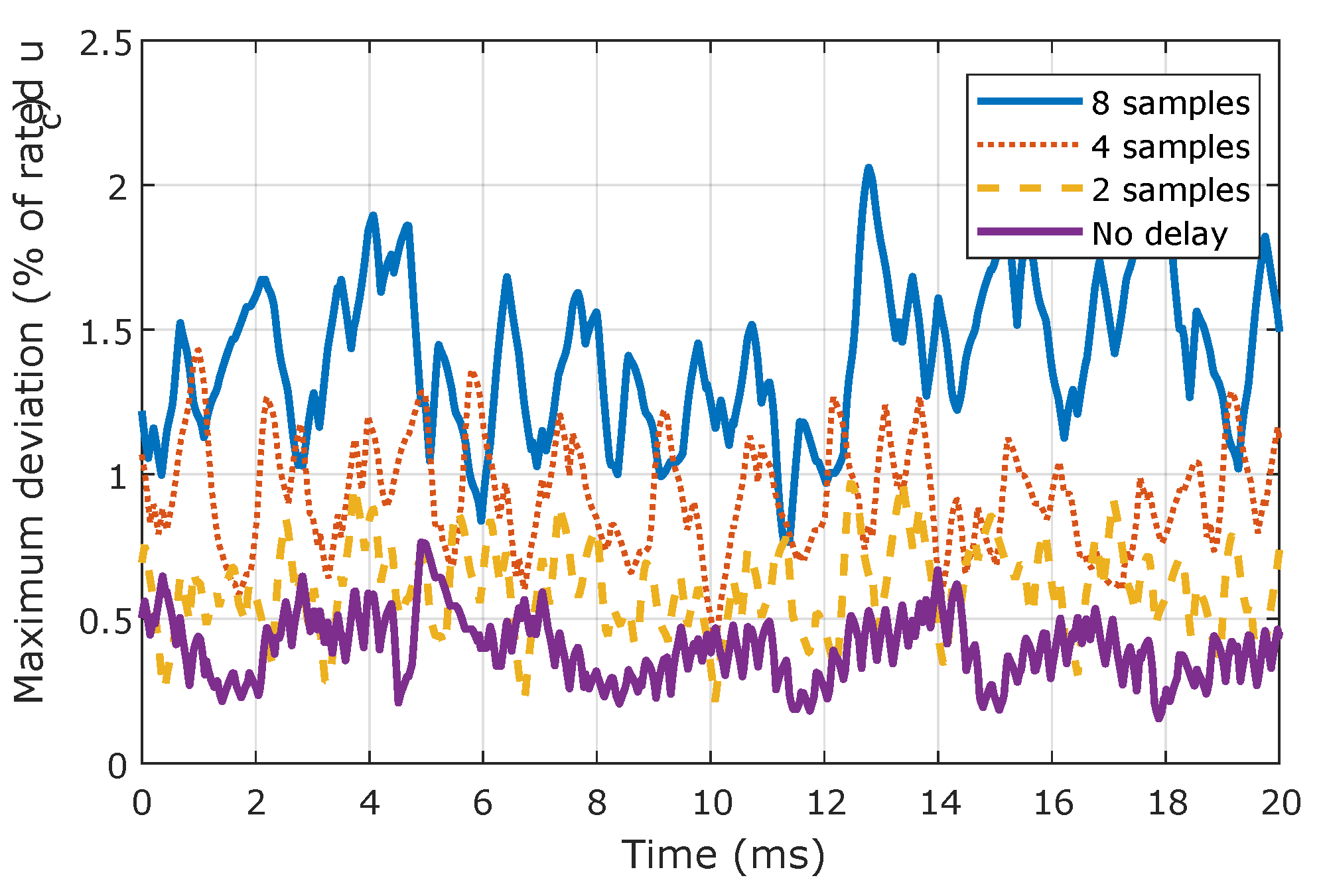
The controller outputs either one reference per cell or single ones per arm, as explained in Section 2. In the case of the first, the control is centralized, and the central unit is responsible for the modulation and capacitor balancing. Due to the network, the central controller receives data delayed by a few samples. We tested if the use of delayed capacitor voltage measurements could still allow an effective balancing when using the sorting algorithm [31]. For that, we run several simulations introducing delays in the capacitor voltage measurements that are fed back to balancing. The results show that the maximum deviation to the average capacitor voltage increases with the number of samples, but the deviation stays within reasonable limits (Figure 9). Therefore, the standard sorting algorithm is an effective balancing strategy when controlling an MMC over a network.

In case the control outputs single setpoints per arm, as adopted in [14] using phase-shifted carrier PWM, the strategy adopted is partly distributed. The central controller runs the current and outer control loops, while the cells execute the modulation and balancing. In such a case, the network does not affect the capacitor balancing because it is run locally at the cells. For this type of control and different strategies to implement it, also refer to [15,16,32].

5. Parameters’ Sensitivity

The estimation algorithm proposed uses a model of the plant, which raises concerns over the system performance and stability as the model and plant deviate from each other.

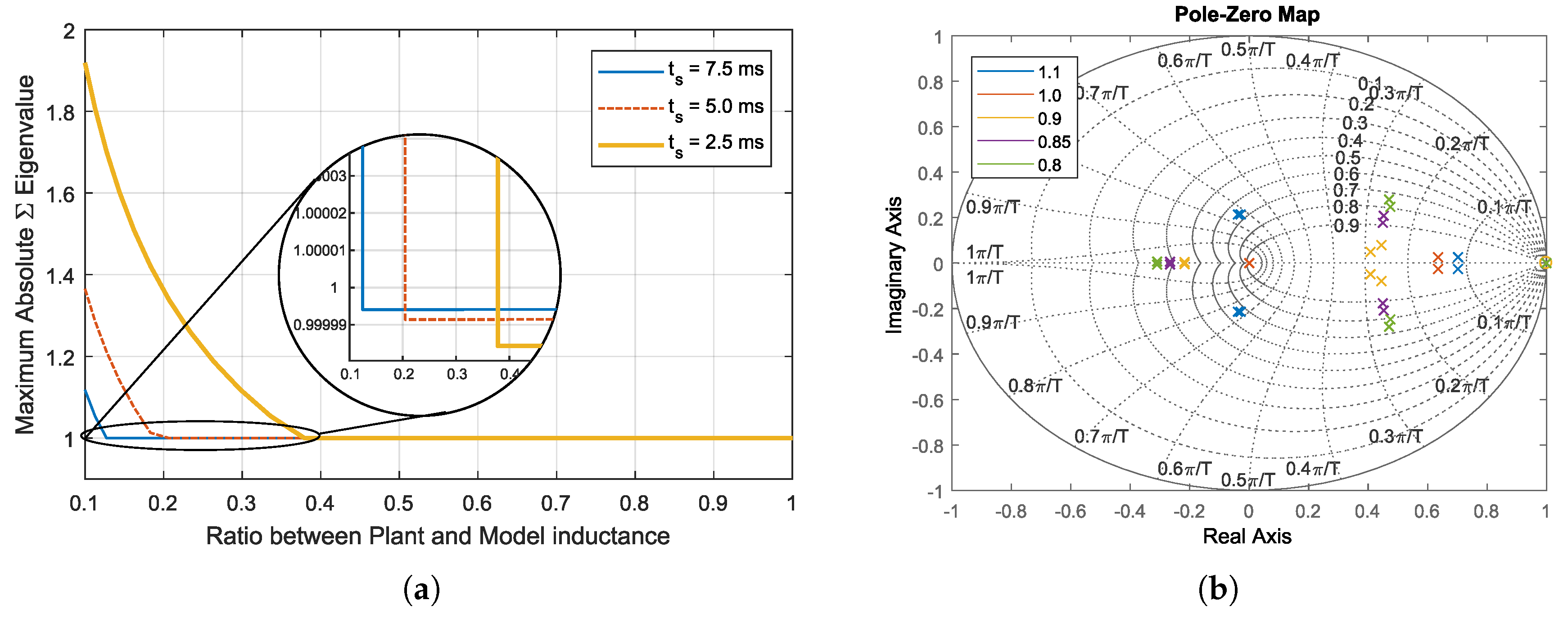
It is possible to verify the system stability, study mismatches between plant and model or the effect of the controller tunning by calculating the eigenvalues of (14) in [21]. To exemplify, we discretized the plant (3) using a Zero-Order Hold and considered the closed-loop system with a delay of two samples (Figure 7). The maximum absolute Eigenvalues of the matrix $\Sigma$ (defined in [21]) for different plant/model inductance ratios ($L_{eq}/{\widehat{L}}_{eq}$) and controllers’ gains, represented here as the settling time used in the controller design, are shown in Figure 10a. As expected, a faster controller is more sensitive to models’ mismatch, but the closed-loop plant is stable with all three controllers as long as the plant to model inductance ratio is greater than 0.38. Note that high voltage MMCs typically use dry-type air-core reactors [28], so errors of this magnitude are unlikely. Furthermore, they are associated with expensive projects that have long implementation periods; hence, a good characterization of the filter components is feasible.

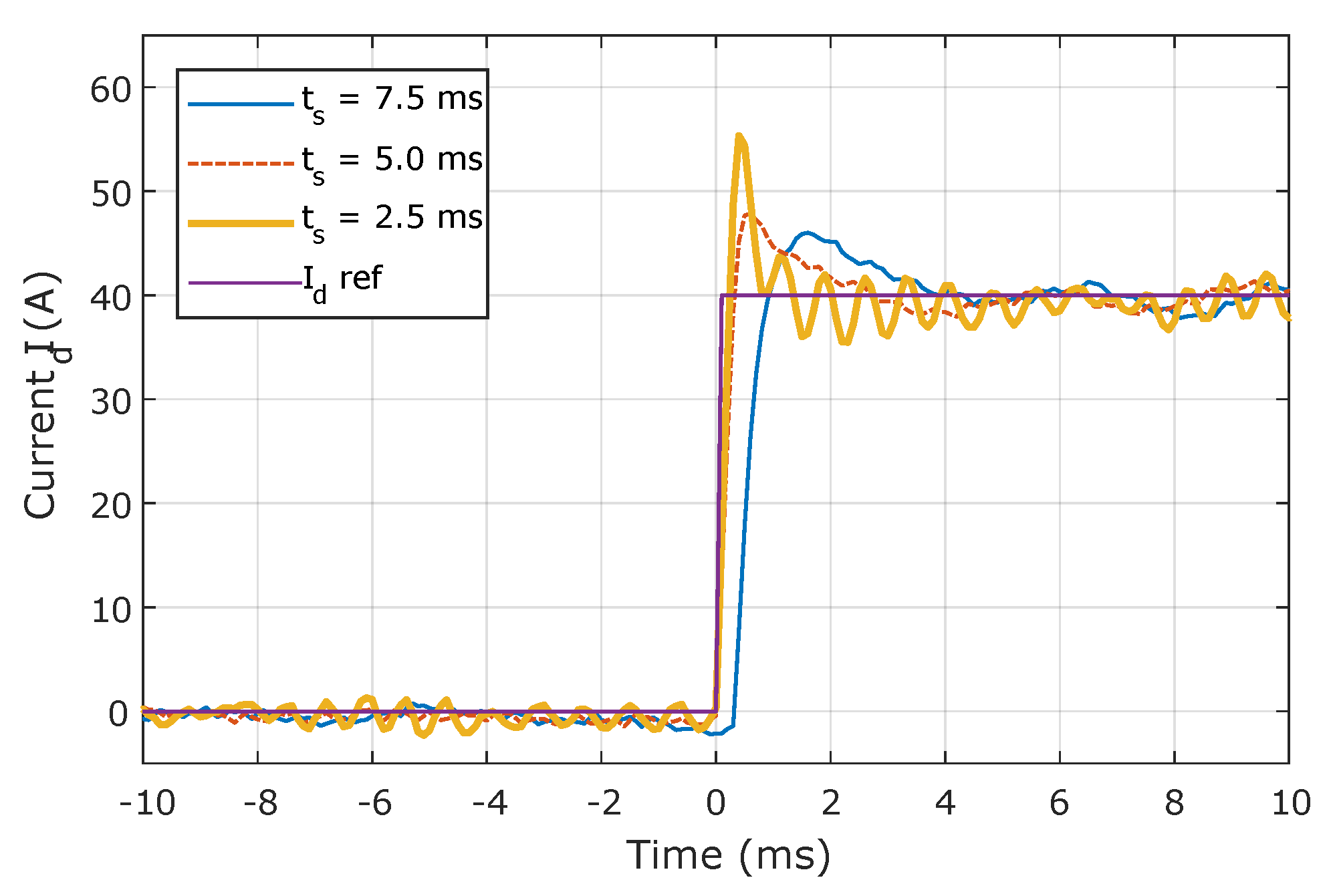
A second method for the verification of the sensitivity to parameters variation is to plot the root locus of the closed-loop plant (14), as in Figure 10b for the controller with $t_s=2.5\mathrm{ms}$. Finally, we show simulation results of a step response for three controllers when the equivalent plant inductance is 0.5 of the model value (Figure 11).

6. Simulation and Experimental Results

We simulated a STATic COMpensator (STATCOM) using a detailed equivalent circuit model (type 4 [33]) in Matlab/Simulink (2017a, Mathworks Inc., Natick, MA, USA) as proposed in [34]. The simulation time with this modeling is about the same as with a full detailed model (type 2 [33]) for small converters, but it simplifies the parametrization of the number of cells and reduces the simulation time of larger converters dramatically.

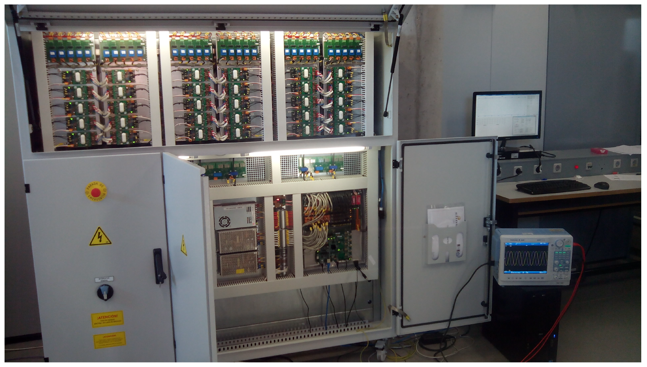
The experimental results were taken using a reduced scale prototype (Figure 12) also working as a STATCOM. It is a quasi-industrial three-phase converter, rated to 50 kVA/400 V, with five half-bridge cells per arm (see Table 1). The control is based in Xilinx Zynq System-on-Chip and can simultaneously measure 43 analog signals, command 64 power switches through fiber optics, and receive 32 fault signals (refer to [35] for a detailed description of the prototype). The Programmable Logic (FPGA) has the following tasks: measure the grid voltage angle with a Phase-Locked Loop (PLL); acquire the data from the Analog/Digital converters; do the modulation that controls the power switches; keep the capacitor voltages balanced (sorting algorithm). The Processing System (ARM cores) has two tasks: execute the control loops and run the server of the data acquisition and supervision system. In our implementation, the time necessary for data conversion is 12.5 µs; for control calculations is 6.5 µs; for system protection is 4.8 µs. The total time for all tasks is 27 µs.

The control architecture of this converter is centralized, i.e., a single hardware unit controls all the cells. For the validation of the proposed method and the sake of simplicity, we emulated the digital communication network by adding a delay of one sample between the output of the control and the PWM. From the control point of view, this is an accurate emulation of a distributed implementation based in a real-time communication that guarantees to meet its deadlines, as long as the links have a low probability of losing or corrupting packets. In total, the system experiences two delays between sampling and actuation, one owing to the digital nature of the controller and the other to the delay introduced by the network.

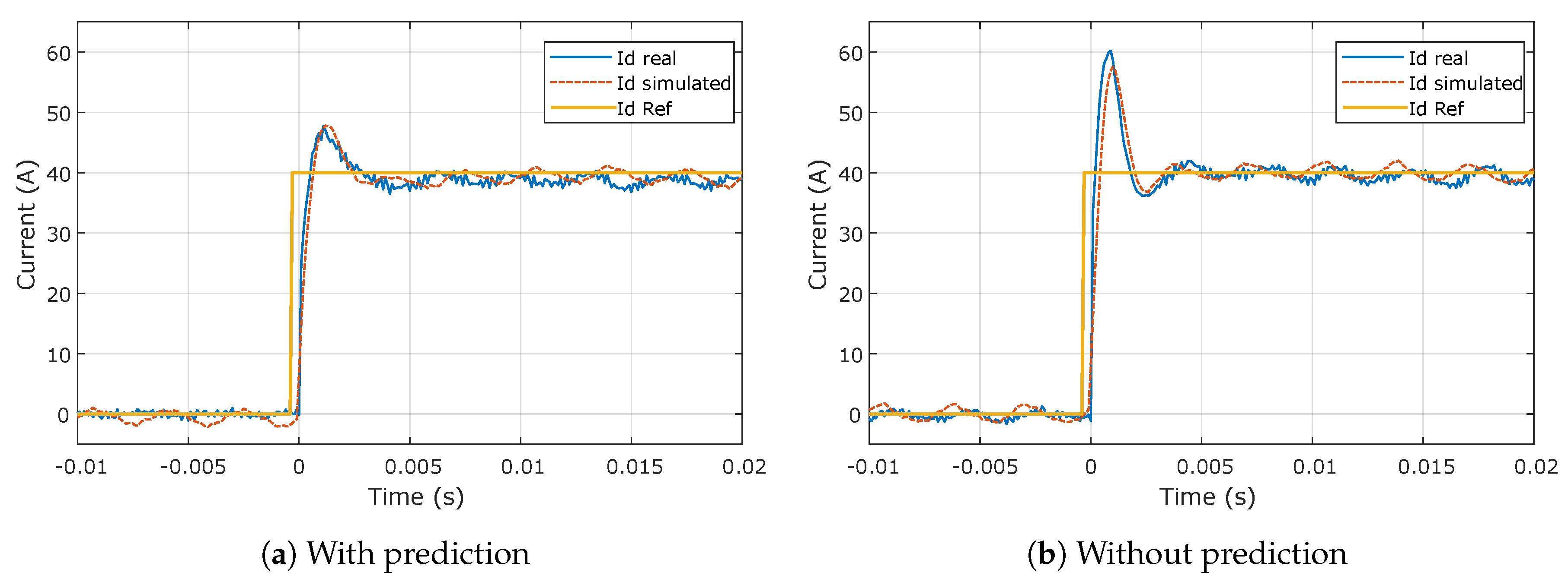
We present the simulation and experimental results in Figure 13 under two different scenarios: (a) with and (b) without the model-based latency compensation. The blue and the dashed orange waveforms are the simulated and experimental response, respectively, to a reference step in the reactive power current $I_d$. In a STATCOM, the current $I_q$ controls the flow of energy to keep the average capacitor voltage at the setpoint; hence, no changes in its reference were carried out.

As expected, the system has a narrower phase margin and the closed-loop response is less damped when the latency is uncompensated, so the overshoot is higher and the settling time is longer. On the other hand, the step response with the compensation has less overshoot and is faster, demonstrating the benefits of the proposed approach.

The simulated and experimental responses are almost identical (see Figure 13), which validates both the model and the model-based compensation strategy. The only tweak needed in the simulation was to include the grid fifth and seventh harmonic, with the magnitude measured at the point of common coupling, and to adjust their relative phase to the fundamental.

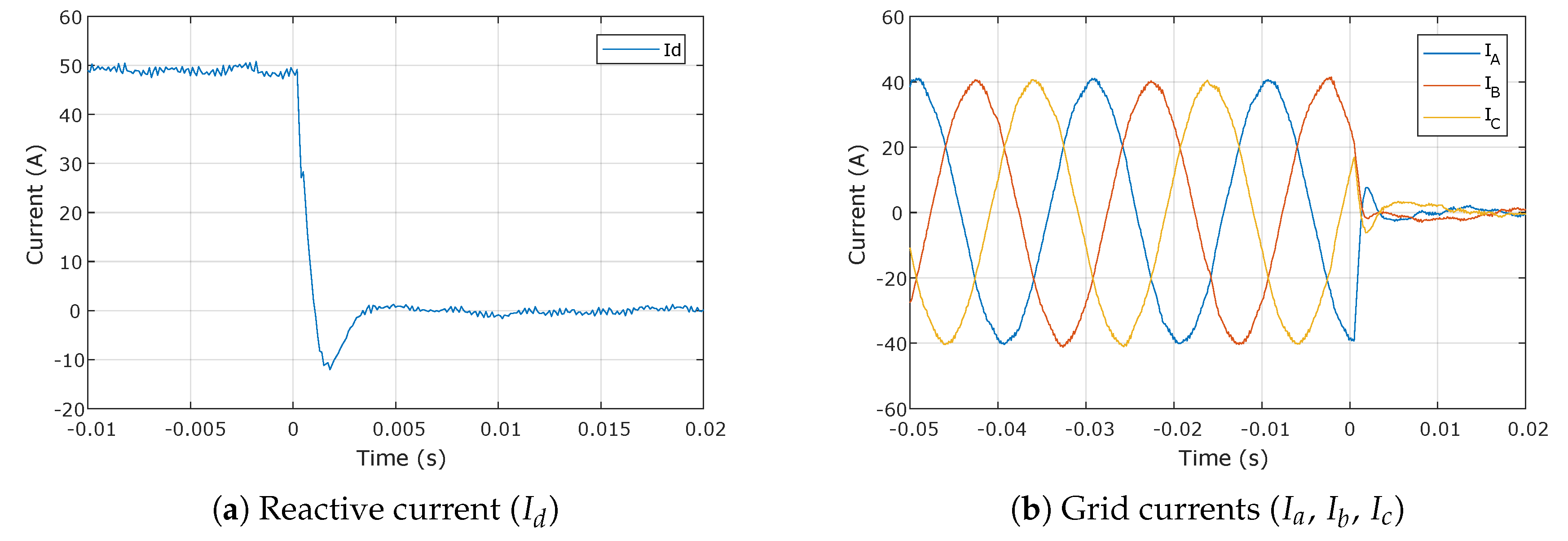
Additionally, in Figure 14a,b, we show, respectively, the reactive and the grid currents when the controller commands a negative current step in a system with a delay of three samples (two from the network and one from the digital control) and that uses the model-based predictor. Note that we do not consider this a real use-case of the proposed method because the designers have the freedom to choose the sampling period and the communication network deployed; we believe that it is better to have a higher sampling period than a loop delay higher than two samples. Despite this consideration, the system response has the same settling time and overshoot as when the network adds a single delay, but without the prediction, the system becames unstable.

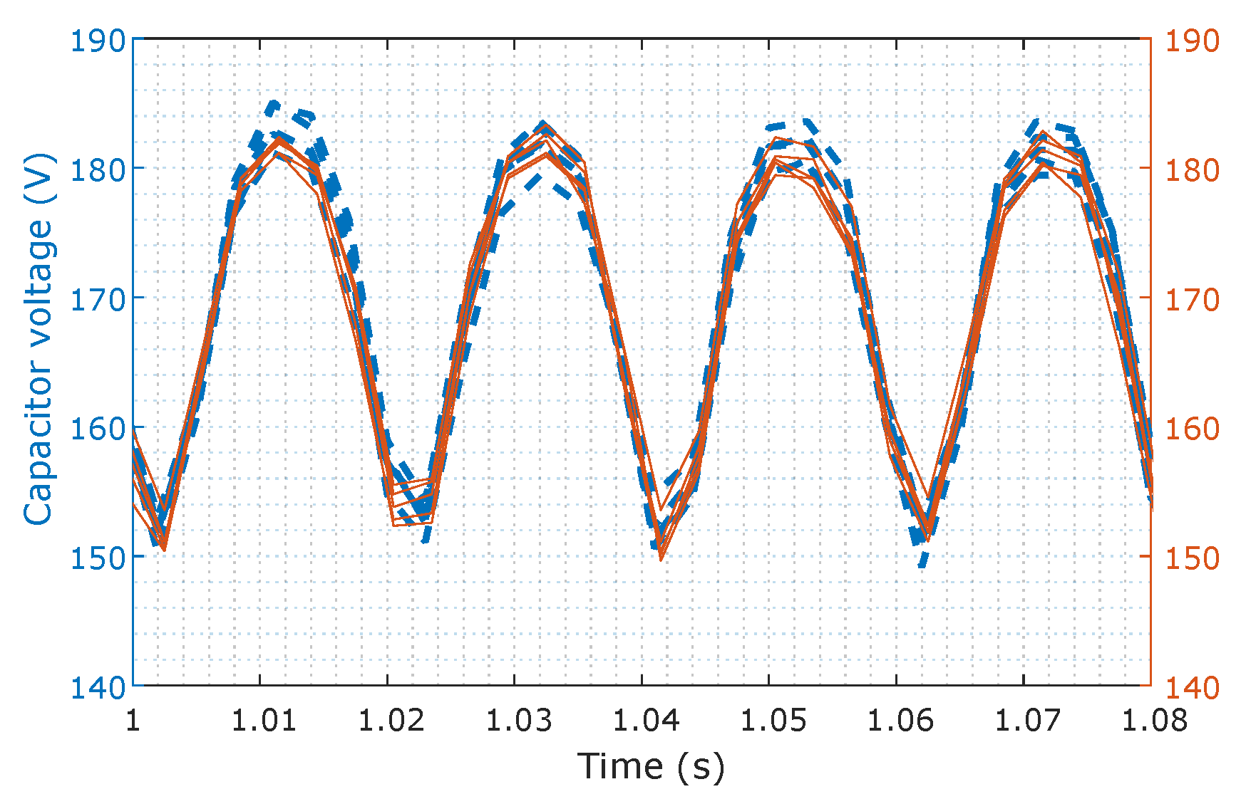
In our experimental setup, the control balances the cell voltages employing the sorting algorithm. For this, it receives from each cell its voltage, organizes the cells in ascending order, and selects the ones with the highest or lowest voltages depending on the arm current polarity. When the converter control has an internal network, the capacitor voltage will reach the central controller after the delay introduced by the network. We have tested the scenario without any delay and emulated a network that delays the capacitor voltages by two samples. Figure 15 shows the measured capacitor voltages from one arm of our experimental converter, where we see that the delay of only two samples does not influence the balancing.

7. Conclusions

The use of a digital communication network into the design of Modular Multilevel Converter introduces a loop delay to the plant, making the controller design harder, reducing dynamic performance, and restricting the minimum sampling period. To the best of our knowledge, researchers have coped with these consequences by minimizing the introduced loop delay. In this work, we adopted a different approach and used a model-based predictor to compensate for the loop delay.

By analogy with the Smith predictor, we can state that the proposed method removes the loop delay from the denominator of the closed-loop transfer function. The PI controller design considers only the delay-free plant [30]. Hence, it can have higher gains, and the transient system response is faster. By accounting for the disturbance effects in the model, it can also improve the disturbance rejection [19].

Moreover, the proposed method allows decoupling the sampling period from the communication Minimum Cycle Time because the system can tolerate longer delays. As a result, either the sampling period can be reduced or a higher Minimum Cycle Time can be tolerated. Thus, the method increases the flexibility in the system design.

We proved the feasibility and better performance of the proposed method using Matlab/Simulink simulation and implementing it in a reduced-scale prototype. Additionally, we assessed the tolerance to parametric variations and found that, for the converter analyzed, the proposed method is robust to mismatches between plant and model.

The results obtained reassure engineers that it is possible to use an internal digital communication network in a Modular Multilevel Converter, with all the advantages in terms of hardware design and ease of implementation/maintenance, while still having flexibility and good dynamic performance.