Composite Harmonic Source Detection with Multi-Label Approach Using Advanced Fusion Method

Abstract

With the integration of clean energy and new power electronic devices into the power grid, the superposition of harmonic sources has become increasingly apparent and common. There is an urgent need to effectively identify composite harmonic sources in the new energy grid. This article proposes a multi-label composite harmonic source classification method that integrates knowledge representation with the transformer model. First, triplets from harmonic monitoring data are extracted and TransR models are used to train time-frequency feature representation vectors. Then, the transformer model is trained to learn the data features of different harmonic sources. Finally, based on the multi-label classification method, composite harmonic sources are identified. This article integrates the semantic information of time-frequency features into the data samples, increasing the interpretability of the model while expanding the inter-class features, which is conducive to the classification and recognition of the model. Compared with other deep learning recognition methods, verification based on simulation data and measured data shows that this method has low training complexity and higher recognition accuracy.

1. Introduction

With the integration of large-scale clean energy and new power electronic devices, the power grid presents randomness and volatility. In addition, there are more diverse types of harmonic sources, and harmonic source recombination is more obvious and common [1,2,3]. The problem of harmonic pollution is becoming increasingly serious, and identifying harmonic pollution sources is an important prerequisite for promoting the effective implementation of harmonic reward and punishment mechanisms and harmonic governance [4]. Therefore, identifying the types of composite harmonic sources in the new power system is of great significance.

Traditional harmonic source identification methods are mainly divided into four categories, as shown in

Table 1. Traditional harmonic source identification method.

Reference	Method	Advantage	Shortcoming
[5]	Harmonic Power Method	Simple and easy to operate.	Prefer to qualitatively explore whether there are harmonic sources in the grid or on which side of the directional analysis.
[6]	Harmonic Impedance Method	Able to consider the impedance characteristics of the system.	Requires accurate harmonic impedance information.
[7,8,9]	Signal Processing Tech	Can handle nonlinear and time-varying signals, suitable for real-time applications.	Sensitive to noise and interference, more sensitive to parameter selection.
[10]	Mathematical Statistics	Provides rigorous analysis and inference of data.	Strict assumptions about data distribution and may not be able to handle nonlinear relationships.

, which are the harmonic power method [5], the harmonic impedance method [6], signal processing technology [7,8,9], and mathematical statistics methods [10]. The harmonic power method is more inclined to qualitatively determine whether there is a harmonic source in the power grid or to analyze whether the harmonic source is a system measurement or a user-side resource. The harmonic impedance method requires accurate harmonic impedance information, which is not easy to collect in actual power systems. To improve the shortcomings of these methods, some scholars have combined signal processing technology and mathematical statistics methods to achieve harmonic source identification. References [7,8,9] classify harmonic sources based on wavelet transform, S-transform, and independent component analysis, respectively. These methods can handle nonlinear and time-varying signals but are sensitive to noise and parameters. Reference [10] uses a mathematical method to identify data from different harmonic sources by establishing a load equivalence model. This method can fit kinds of data well, yet it is difficult to solve the nonlinear relationship and has poor linear generalization.

However, neither of the above methods can identify the specific type of harmonic source. In addition, these research ideas have the following problems:

• The factors that generate harmonics in the new power system are complex. It is more difficult to grasp the harmonic generation mechanism and construct a harmonic source identification model comprehensively and accurately, and it is less practical and adaptable.
• The method based on mechanism analysis does not make full use of the massive data generated by intelligent monitoring equipment in the era of big data, and the fitting results cannot reflect all the information of the harmonic source [11].
• Some data are not easy to obtain, e.g., harmonic impedance, harmonic phase angle, and topology cannot be directly obtained from the monitoring device.

To sum up, the traditional harmonic source mechanism method is limited to apply. Nevertheless, machine learning models can break down the barriers of electrical mechanisms and compensate for the shortcomings of mechanical methods. Machine learning models are superior to traditional methods in harmonic analysis [12], especially when operating condition changes. For example, reference [13] used the improved Fourier and artificial neural network to extract the amplitude and frequency characteristics of harmonic signals and realized the classification and identification of multi-harmonic sources by constructing a random forest model. Reference [14] extracted the relationship between the spectrum data of harmonic voltage and current based on the neural network model. Based on the derived dynamic parameter model, harmonic sources can be identified. Reference [15] fused random forest and long short-term memory (LSTM) models to extract features from harmonic time series data. Thus, machine learning models can successfully identify harmonic sources in high precision, which brings significant advantages to the research field.

However, with the development of smart grids, the harmonic monitoring data obtained at a certain monitoring point are often the result of the joint action of multiple harmonic sources. This means it is dangerous to ignore the harmonic pollution caused by convoluted decentralized harmonic sources. The above methods cannot meet the practical needs to classify or identify the single source [3]. Therefore, it is of great theoretical value and practical significance to study the method of identifying composite harmonic sources.

In summary, the existing harmonic source identification methods usually assume that the harmonic source data contain only a single category. Moreover, these methods are incomplete in feature extraction and rarely cover both time-domain and frequency-domain models. For example, references [13,14] only extracted the frequency-domain features of harmonic data, while reference [15] only extracted time-domain features. In response to the above problems, this paper proposes a new harmonic source identification method. Based on the two dimensions of time and frequency, a multi-label classification model that integrates TransR knowledge representation and the transformer model is designed, referred to as TransR-transformer-multi-label (TTM).

The transformer model is a type of deep neural network architecture introduced in the paper “Attention is All You Need” by Vaswani et al. in 2017 [16]. It is designed for sequence-to-sequence tasks, such as machine translation, and relies on self-attention mechanisms to capture dependencies between input and output data [17,18], which can effectively capture the sequence features of harmonic data from the global scale. Therefore, the transformer model can simultaneously extract the time-frequency characteristics of harmonic source data. Applying the transformer model to the harmonic source identification of new power systems greatly improves the identification accuracy. TransR is a knowledge representation method used in machine learning [19]. It embeds entities and relationships into a continuous vector space to capture semantic relationships. Since the coupling conditions between multiple harmonic sources are complex and changeable, the difference in characteristics between the composite harmonic sources will be reduced after the harmonic data are superimposed or reduced. Therefore, this paper introduces a knowledge representation method to expand the inter-class differences of composite harmonic data. The multi-label classification method has an advantage in solving the problem of composite perturbation classification [20,21]. The pattern classification is carried out by the multi-label classification algorithm, which has higher recognition accuracy and generalization ability. This paper uses a multi-label classification method to decouple composite harmonic source data, which can accurately identify the components of unknown harmonic sources.

The innovation of the TTM model proposed in this article lies in the characteristic analysis of harmonic source data from two new perspectives. One is to extract time-frequency features of harmonic data simultaneously, and the other is to extract semantic features of harmonic source data and generate knowledge representation vectors for model training. In addition, identifying the components of composite harmonic source data lays the foundation for further solving the problems of harmonic traceability and responsibility division of multiple harmonic sources. Finally, real data and simulated data were used to verify the high accuracy and strong generalization of the model.

The follow-up outline is as follows:

Section 2: New perspective on harmonic source characteristic analysis. This section explores an innovative approach to harmonic source analysis, introducing a fresh methodology and theoretical framework.

Section 3: Identification method of composite harmonic source based on TTM. This section introduces the design ideas and overall architecture of the TTM model.

Section 4: Analysis. This section explains how to train the model and analyze the results on real data.

Section 5: Simulation. This section adds a practical dimension by discussing simulated scenarios and outcomes, validating the proposed identification method in controlled environments. Simulation results serve to reinforce the reliability and applicability of the TTM-based approach.

Section 6: Discussion. By synthesizing findings, this section concludes and critically discusses research implications, contributing to harmonic source characteristic analysis.

Section 7: Conclusions. The last section summarizes the innovations of the method proposed in this article and emphasizes its contribution to the analysis of harmonic source characteristics.

2. New Perspective on Harmonic Source Characteristic Analysis

This article proposes a new perspective on harmonic source characteristic analysis. One is to consider both the time domain and frequency domain dimensions, which can obtain harmonic characteristics more comprehensively and accurately and achieve accurate identification of composite harmonic sources. Another perspective is to introduce knowledge representation methods, extract semantic features of harmonic data and generate semantic representation vectors, enrich harmonic data features, and increase inter-class differences of composite harmonic sources.

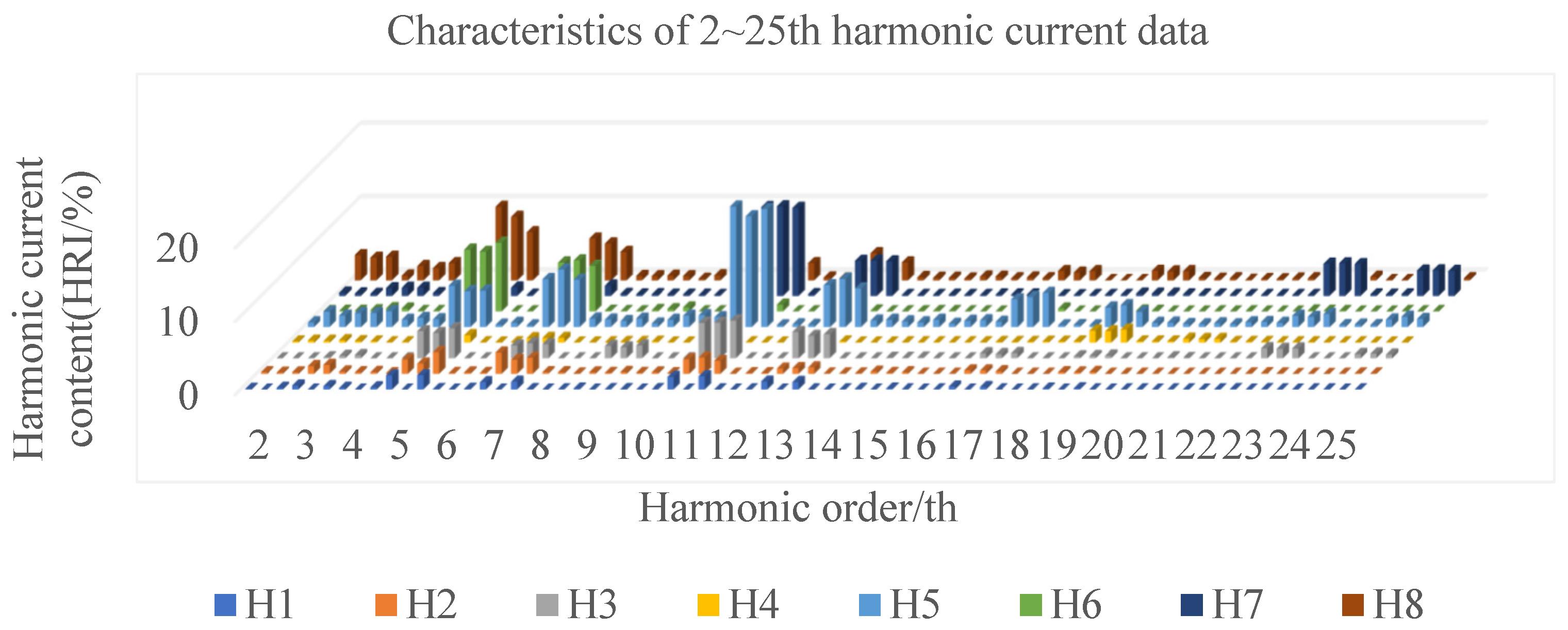
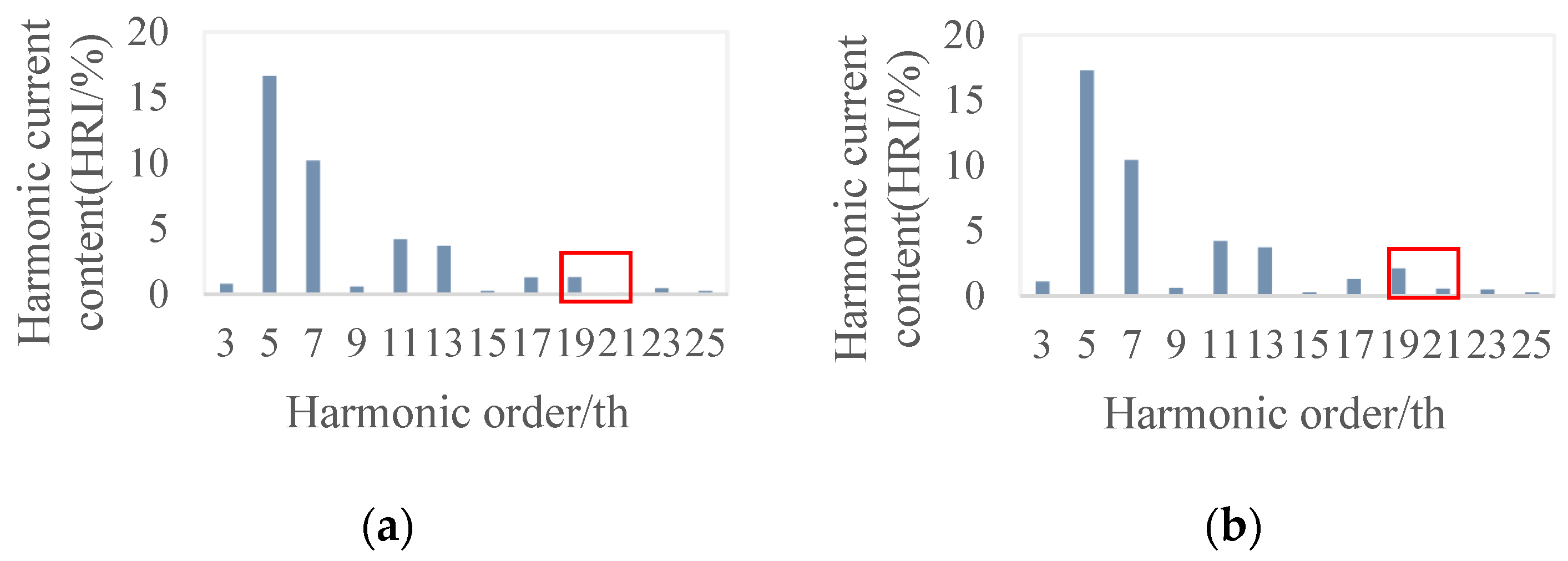
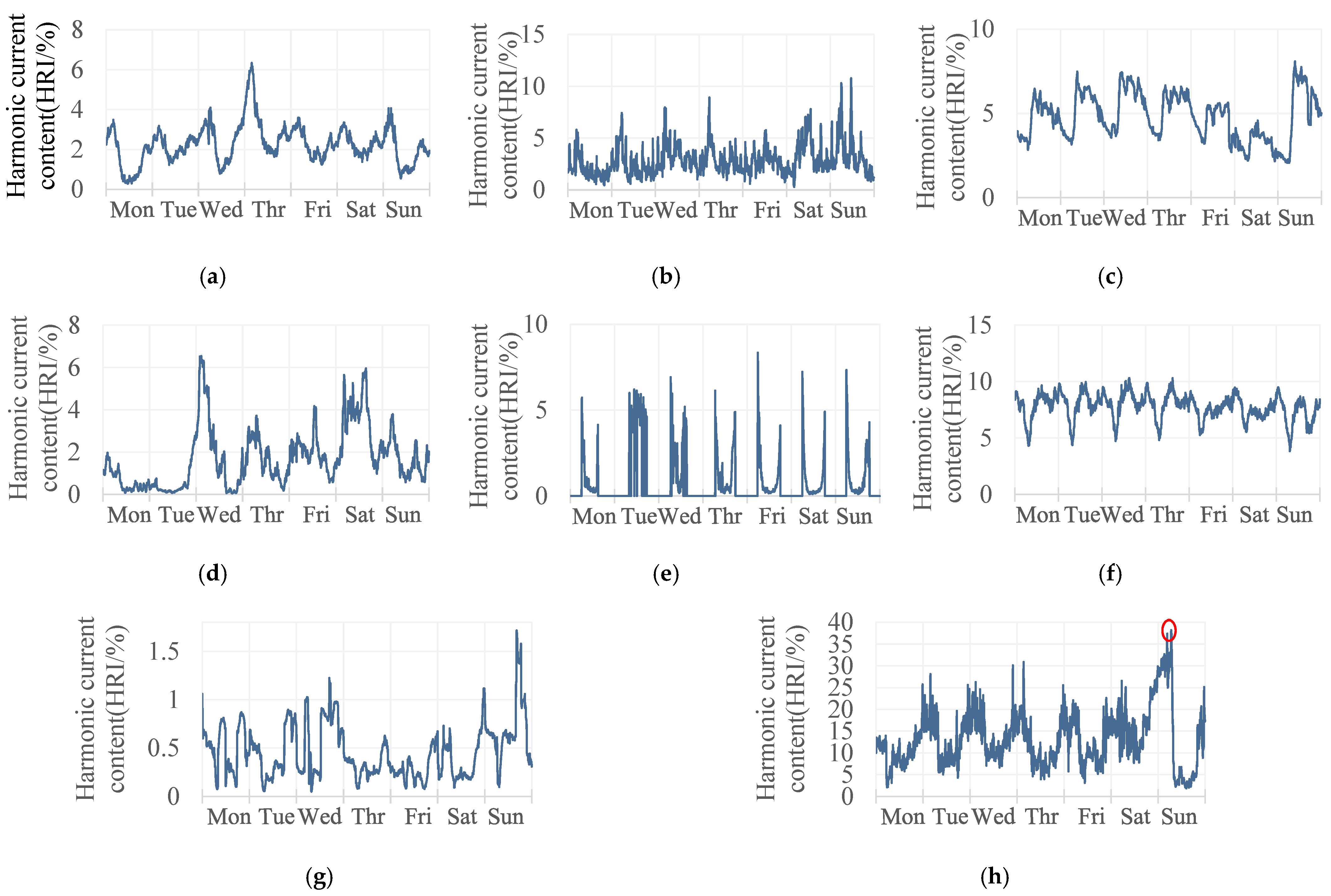
2.1. Time-Frequency Characteristics of Harmonic Sources

Harmonic pollution is widespread and exists in multiple processes of power generation, transformation, transmission, distribution, and consumption in the power system. The frequency-domain characteristics of harmonics generated by different harmonic sources and their fluctuation trends over time are different. Figure 1 shows the data characteristics of 2–25th harmonic currents from eight harmonic sources sampled at a certain time, including electric vehicle charging station (H₁), electric heating load (H₂), electrified railway (H₃), wind farm (H₄), photovoltaic (H₅), rail transit (H₆), converter grid side (H₇), and rolling mill (H₈). The horizontal axis represents the harmonics of the three-phase current data. The vertical axis represents the content of each harmonic current, that is, the percentage of harmonics in the effective value of the fundamental current. The larger the ordinate value, the greater the impact on harmonic generation. From Figure 1, the harmonic current content of H₅, H₆, H₇, and H₈ is high. The 11th harmonic content on the H₅ and H₇ is the highest, with H₅ around 16% and H₇ around 12%. The 5th harmonic current content of H₆ and H₈ is the highest, both approximately 10%. It can be concluded from the figure that the frequency domain characteristics of different harmonic sources in the new power system are different, so the frequency domain characteristics of each harmonic source need to be learned separately.

From Figure 1, each harmonic source has a relatively prominent harmonic order. The contribution value of a certain harmonic to the total harmonic current distortion [22], denoted as I_m, is defined to determine the number of harmonics that cause harm in each harmonic source.

$$I_m=\frac{I_x}{\sqrt{{\displaystyle \sum _{h=2}^{\infty }{I_h}^2}}},$$

(1)

where I_x represents the value of any harmonic current, and the denominator represents the content of all harmonic currents. The I_m of the eight harmonic sources in Figure 1 is calculated and then I_m is compared to the corresponding curve graphs of the harmonic source data. The results, depicted in

Table 2. Contribution values of odd harmonics from different harmonic sources.

Harmonic Order/th	Im
	H1	H2	H3	H4	H5	H6	H7	H8
3	0.173	0.245	0.018	0.153	0.094	0.017	0.073	0.049
5	0.624	0.453	0.482	0.487	0.277	0.781	0.074	0.734
7	0.329	0.674	0.230	0.277	0.321	0.619	0.099	0.418
9	0.044	0.048	0.223	0.041	0.057	0.018	0.014	0.043
11	0.564	0.466	0.631	0.041	0.805	0.069	0.844	0.298
13	0.354	0.170	0.469	0.056	0.281	0.020	0.333	0.271
15	0.025	0.073	0.010	0.023	0.032	0.007	0.012	0.019
17	0.132	0.111	0.088	0.041	0.186	0.027	0.009	0.093
19	0.044	0.056	0.033	0.754	0.131	0.010	0.022	0.096
21	0.004	0.005	0.016	0.247	0.019	0.003	0.009	0.007
23	0.015	0.012	0.180	0.033	0.076	0.012	0.306	0.034
25	0.010	0.008	0.076	0.018	0.052	0.006	0.240	0.019

, indicate that the I_m values of the relatively prominent harmonic orders from various sources exceed 0.1. For example, in Figure 1, the 12K ± 1 (K = 1, 2) harmonic on the converter network side is dominant, and the main harmonic of the rolling mill is 6K ± 1 (K = 1, 2). Therefore, we define the main harmonic order when its I_m is over 0.1. In addition, it can be concluded from Table 2 that, although the main harmonic orders of H₁ and H₂ are the same, the main harmonic orders of other harmonic sources are different. Although H₆ and H₇ both have only two major harmonic orders, they correspond to 5th and 7th, and 11th and 13th, respectively. Hence, analyzing the semantic features reflected in this data, such as the characteristics of harmonic sources, will aid in the classification and identification of models.

In the case of single-point measurement, the frequency-domain characteristics of different harmonic sources are more obvious and easier to distinguish. However, due to the complexity of power lines in the power system, harmonic distortion at common connection points is the result of the combined action of multiple harmonic sources. The harmonic currents generated by different harmonic sources mutually enhance or cancel each other, causing changes in harmonic frequency and interfering with the identification of composite harmonics.

For example, Figure 2 shows two different composite harmonic source data, but the data characteristics are very similar. Differentiating between Figure 2a,b visually is challenging; however, they do possess distinct features. The red box serves as a highlight, and there are significant differences between the two images in the red box area. Notably, in Figure 2a, the amplitudes of the 19th and 21th harmonics appear smaller compared with those in Figure 2b. Figure 2a is the harmonic source coupled by a rail transit and rolling mill, and Figure 2b is the composite harmonic source of a wind farm superimposed based on Figure 2a. Specifically, although the harmonics of the wind farm have a small impact on the overall harmonic source data when harmonic pollution occurs, each harmonic source may have a certain impact on the results. Particularly in the case of compounding, the superposition of individual harmonic sources may lead to more complex data characteristics. This similar but slightly different situation of composite harmonic source data makes the task of harmonic source identification somewhat challenging. It requires a model that can accurately capture and distinguish these subtle differences to improve the ability to accurately identify complex harmonic sources.

Taking the 5th harmonic current as an example, Figure 3 shows the fluctuations of the above eight harmonic sources for one week. It can be seen from the figure that there are significant differences in the fluctuations of different harmonic sources over time. H₈, as a high-energy-consuming harmonic source, has a harmonic content rate much greater than other harmonic sources. The red circle highlights a maximum value in Figure 3h. Its harmonic content rate on Sundays can exceed 35%, which may seriously affect the stable operation of the system. Among these harmonic sources, H₅ has relatively special properties. Affected by light, photovoltaic harmonics concentrate on a certain period of the day, and no harmonics generate the rest of the time. The daily harmonic current data of H₃ and H₆ show periodic fluctuations with certain regularity. In contrast, other harmonic sources’ daily harmonic current data show different fluctuation trends and lack obvious periodicity, making feature extraction of harmonic current data more challenging. For harmonic sources with these properties, it is necessary to adopt more flexible and targeted analysis methods. Therefore, integrating the time characteristics of harmonic data into model training can enrich the features of different harmonic source types and improve the identification ability of the model.

In summary, there are certain limitations in identifying frequency-domain or time-domain features alone. Due to incomplete feature extraction, this may lead to a reduction in recognition accuracy. Therefore, it is necessary to analyze time-frequency characteristics simultaneously. This comprehensive analysis method contributes to a more comprehensive and in-depth understanding of harmonic problems and provides a more reliable basis for effective harmonic source identification. Through time-frequency characteristic analysis, we can more accurately capture the changing patterns of harmonic sources in different time scales and frequency ranges, improve identification accuracy, and provide stronger support for harmonic control in power systems.

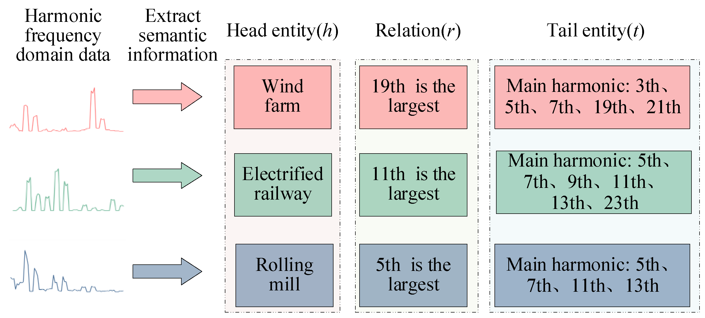
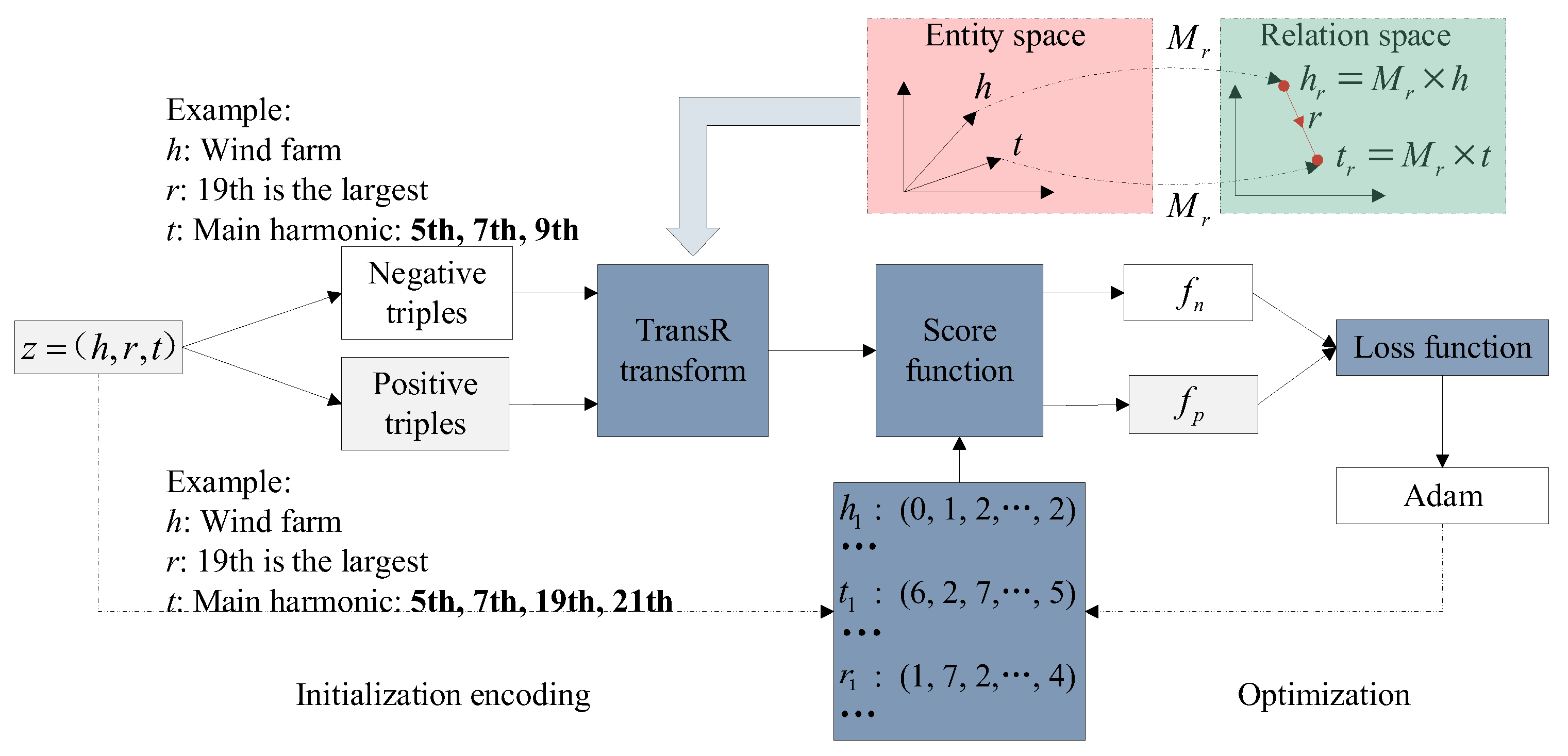
2.2. TransR Knowledge Representation

The existing power quality monitoring network has been widely deployed in power grid companies, accumulating massive harmonic time-domain and frequency-domain data. These data contain rich semantic information and prior knowledge, but discrete and structured data cannot be directly used for machine learning model training. Therefore, discrete semantic features are extracted through triplets and knowledge representation algorithms are used to map the knowledge patterns contained in discrete data to a low dimensional vector space [19]. Then, the formed vector data are input into the transformer model for training. The semantic features of harmonic current data can be integrated into the identification model of composite harmonic sources through the above conversion method.

In the Trans series that maps entity relationship triplets to low dimensional space vector representations, TransR can better handle one-to-many and many-to-many relationships and has stronger semantic expression ability [23]. This article is based on TransR to represent the frequency-domain features of eight different time series of harmonic sources as part of the input of the transformer model. It can amplify the feature differences between data samples, standardize the self-attention mechanism, increase the model’s expression and inference abilities, and promote the identification of composite harmonic sources. The data input format for TransR is usually a triplet, with each triplet consisting of head entity, relationship, and tail entity, which can be represented as (h, r, t). Each harmonic datum contains a lot of attribute information, and multiple triplets can be extracted according to actual needs. This article mainly focuses on the characteristics of the main harmonic order of different harmonic sources. The knowledge representation of harmonic source data mainly involves the three processes.

In the process of extracting semantic features and constructing triples, Figure 4 illustrates a triplet derived from the odd harmonic data of diverse harmonic sources recorded at a specific time. Within this triplet, the head entity denotes the type of harmonic source, while the tail entity represents the associated main harmonic order. The relationship between them indicates the maximum harmonic order, identifying the harmonic order with the highest current content. Semantic information is extracted from n harmonic data samples X and entity relationship triplet Z is constructed, where each z consists of (h, r, t).

Then, the TransR model is trained to generate semantic representation vectors. In Figure 5, the training process of the TransR model is delineated into multiple steps. Initially, a collection of positive and negative triples is formed based on each input triplet. The input sample constitutes a positive triplet, while the negative triplet retains the head entity of the positive triplet but substitutes either the tail entity or the relationship with a different tail entity from the dataset. Subsequently, an initial TransR transformation is conducted separately on the positive and negative triples to convert the entity space into a relational space. Then, the converted positive and negative triples are input into the distance score function, respectively, the distance between vectors in the relationship space is calculated, and the scores f_p and f_n are obtained. The distance score function formula [24] is:

$$f(h_r,r,t_r)=\left|\right|h_r+r-t_r\left|\right|,$$

(2)

where h_r and t_r are the representation vectors of the relationship space. The head and tail entities are translated into the spatial dimensions of the relationship r for comparative analysis. The score function’s smaller value indicates a stronger correlation between the head entity and the tail entity in the relationship space. Essentially, this implies a higher correlation between a specific harmonic source and its corresponding main harmonic order, as well as the maximum harmonic order. Conversely, a larger score function indicates a weaker correlation between these entities.

Finally, the Adam optimizer continuously learns and optimizes based on the value of the loss function, and obtains an entity set and a relationship set with semantic information. Different entities and relationships have unique vector representations and contain corresponding semantic relationships. Among them, the loss function formula [24] is:

$$Loss=\max (0,f_p-f_n+\mathrm{margin}),$$

(3)

where the margin is a predefined boundary value used to distinguish the gap between positive and negative triples. The score function shows that f_p is smaller than f_n, and the max function can separate positive and negative triples to the greatest extent. When the gap between f_p and f_n is less than the margin, a positive loss is generated, and the model continues to be encouraged to increase this gap to reduce the loss value. When the gap is greater than or equal to the margin, the loss is zero, indicating that the model has met the boundary requirements. During the iterative optimization process, the loss function continuously weakens the characteristic relationship between the harmonic source type of the negative sample and its corresponding main harmonic order and strengthens the correlation between the head and tail entities and relationships of the positive sample. This helps the model learn better embeddings for similarity or distance measurement tasks.

Finally, the harmonic data features are fused to obtain time-frequency feature vectors with semantic information. Due to the different entities and relationship vectors corresponding to different harmonic source data, the problem of similar current data characteristics caused by different composite situations of multiple harmonic sources has been solved, further expanding the differences between data, and facilitating the identification of composite harmonic source data by the model.

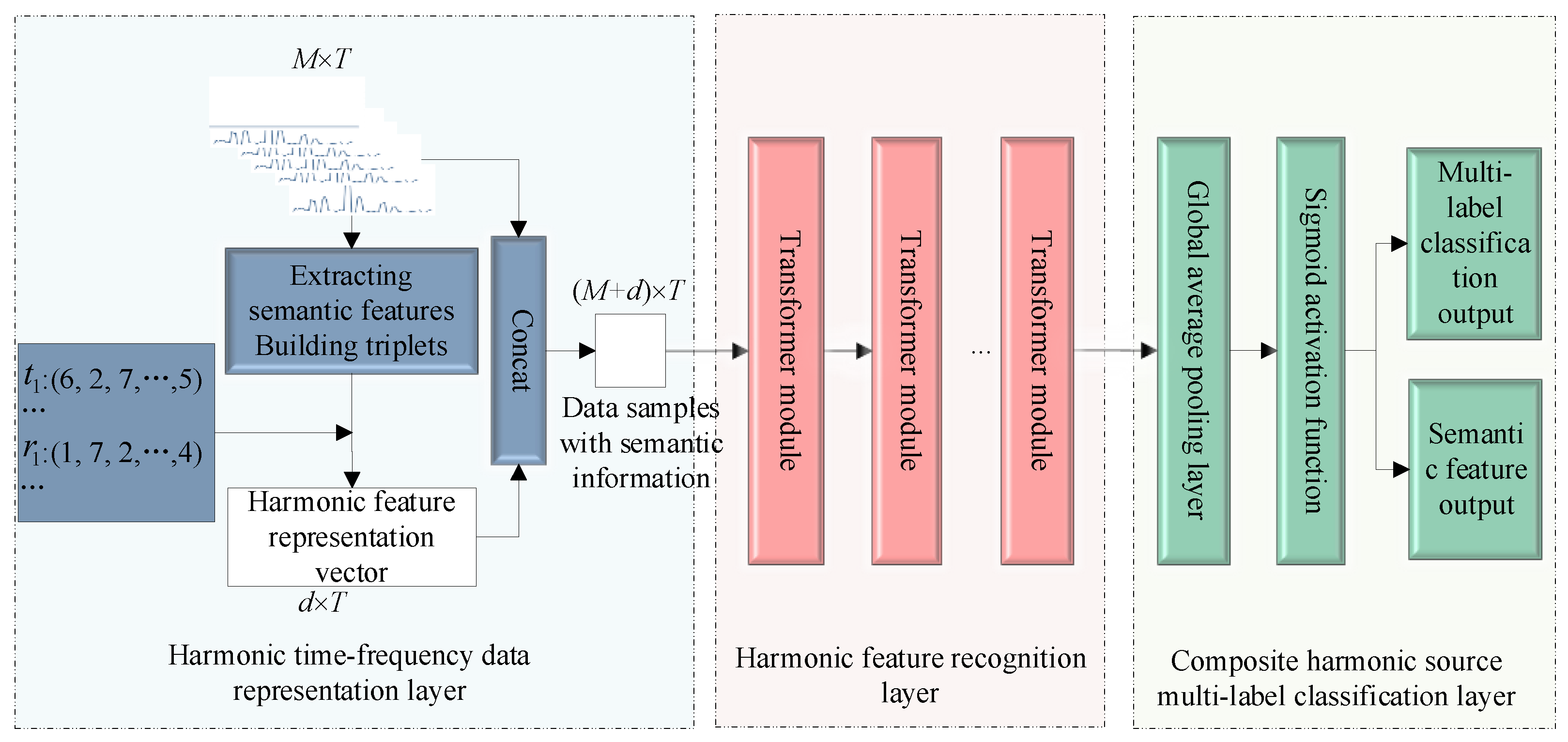
3. Identification Method of Composite Harmonic Source Based on TTM

The traditional transformer model consists of an encoder and a decoder. To achieve the identification of composite harmonic sources, this paper designs an improved TTM model. Due to the transformer model’s focus on feature extraction of time series at the global scale, it is not possible to achieve time-frequency analysis of composite harmonic source data. This article integrates the TransR knowledge representation model to extract local frequency domain features of harmonic current data and generates time-frequency data samples with semantic information to achieve time-frequency domain feature extraction of harmonic current data. At the same time, the multi-label classification model will replace the decoder part of the transformer model to achieve decoupling identification of composite harmonic source data and output a single harmonic source type contained in the composite harmonic source data.

Figure 6 depicts the TTM multi-harmonic source identification network, which comprises the following three main components: a harmonic time-frequency data representation layer, a harmonic feature recognition layer, and a composite harmonic source multi-label classification layer. The network operates as follows.

Specifically, concatenating the representation vectors with semantic information with input samples yields a dataset with time-frequency characteristics. In the input samples, M is the frequency-domain characteristic corresponding to each harmonic of the monitoring data, and T is the time-sequence characteristic. The semantic features of harmonic data are extracted at each time step, and the entity relationship triplets (h, r, t) are constructed. Since the type of harmonic source is unknown, only tail entity and relationship features can be extracted based on known harmonic current data, resulting in a harmonic feature representation vector d containing only relationship vectors and tail entity vectors. The time-frequency data samples with semantic information obtained from the previous layer serve as input samples for the harmonic feature recognition layer. This layer processes the sample set using a multi-layer transformer network. Through iterative training, the network learns data features of different harmonic sources, generating feature vectors. The composite harmonic source multi-label classification layer decouples feature vectors through a multi-label classification process. It includes a global average pooling layer and a sigmoid activation function. The output of this layer presents the single harmonic source types and corresponding semantic features that may be present in the composite harmonic source data, thereby enabling the identification of composite harmonic sources.

3.1. Harmonic Time-Frequency Data Representation Layer

A multi-label classification model based on a transformer model can achieve the classification and recognition of composite harmonic sources. However, due to the small differences between the time domain and frequency domain of the composite harmonic data, it is difficult to distinguish, resulting in poor identification performance of the model. Therefore, this article embeds a harmonic time-frequency data representation layer before the input of the transformer model. The harmonic time-frequency data representation layer provides rich semantic information and relationship representation, which can fully extract time-frequency features, increase the model’s expression and inference capabilities, and improve model performance.

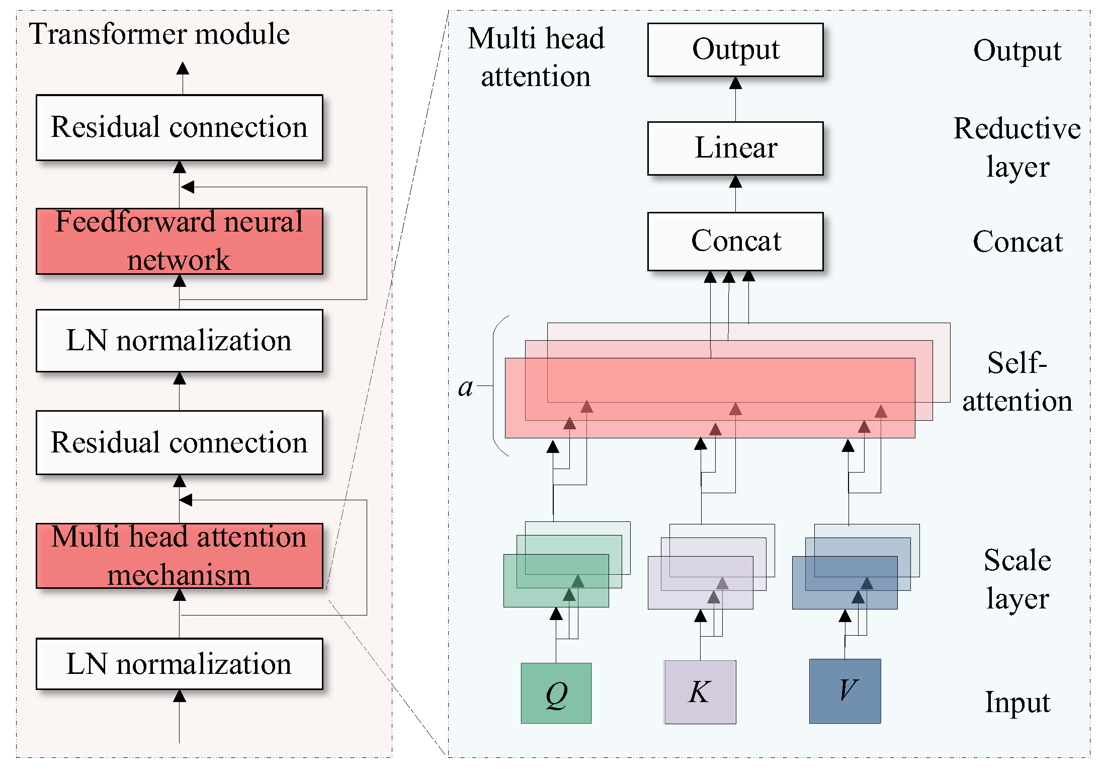
3.2. Harmonic Feature Recognition Layer

The harmonic feature recognition layer consists of multiple transformer modules with the same structure. The input of the first module is the output of the harmonic time-frequency representation layer, and the output of each subsequent module serves as the input of the next module. Multiple transformer modules share a set of parameters, which can effectively capture the temporal characteristics of harmonic sequence data. The internal structure of the transformer module is shown in Figure 7. Each module mainly consists of a multi-head attention mechanism and a feedforward neural network, followed by residual connections and LN normalization.

The multi-head attention mechanism includes a parallel scaling dot product self-attention layer; each layer is called a head. The parameters of each magnetic head are different, and various characteristics of harmonic sources can be learned in parallel from multiple representation spaces. The formula of the multi-head attention mechanism [16] is as follows:

$$\mathrm{MultiHead}(Q,K,V)=\mathrm{Concat}(hea{d}_1,hea{d}_2,\dots ,hea{d}_a)\times W^o,$$

(4)

where Q = K = V and are equal to the input of the multi-head attention mechanism. W^o is a learning parameter responsible for restoring data to its original dimension, ensuring that the input and output dimensions of the multi-head attention mechanism are consistent. Head_i (i = 1, 2, 3,…, a) represents the output of the ith head, while concat represents concatenating the outputs of all heads together.

Each head is the output of the scaled dot product self-attention mechanism, and the head formula [16] is as follows:

$$\begin{array}{c}\mathrm{Attention}(Q_i,K_i,V_i)=\mathrm{softmax}(\frac{Q_i·{K_i}^{\mathrm{T}}}{\sqrt{l}})·V_i\\ Q_i=Q\times W_i^{\mathrm{q}}\\ K_i=K\times W_i^{\mathrm{k}}\\ V_i=V\times W_i^{\mathrm{v}}\end{array},$$

(5)

where Q_i, K_i, and V_i are the three inputs of the self-attention mechanism, corresponding to query, key, and value, respectively. W^q, W^k, and W^v are learnable weight matrices that function opposite to W^o and are responsible for projecting input data into a low-dimensional space. Each self-attention mechanism corresponds to a different weight matrix. q, k, and v are fixed values, and after linear transformation of the weight matrix, the three inputs of the self-attention mechanism are obtained. Firstly, the correlation index is obtained by dot product operation using the transpose of Q_i and K_i. SoftMax normalization is performed to ensure that the total attention weight is 1. Finally, the weighted sum is V_i. Among them, l is the output dimension of each layer, also known as the scaling factor, to prevent gradient vanishing during SoftMax calculation.

The difference between the self-attention mechanism and the traditional attention mechanism is that its queries, keys, and values are all obtained from the same sequence. The self-attention mechanism can simultaneously consider all positions in the sequence and dynamically adjust attention weights based on different inputs. Multiple self-attention mechanisms run in parallel, achieving simultaneous attention computation of harmonic time-frequency data and all positions in semantic feature sequences from multiple representation spaces. Improving the expression ability and feature extraction ability of the model is beneficial for the identification of composite harmonic source data.

3.3. Composite Harmonic Source Multi-Label Classification Layer

To solve the problem of identifying composite harmonic sources and clarify the specific coupling situations of different types of harmonic sources, it is necessary to introduce a multi-label classification model. Multi-label classification is one of the more difficult classification problems, as it allows samples to belong to multiple categories at the same time. This article combines a neural network model for analysis, replacing the decoder part of the transformer model with a multi-label classification algorithm, and achieving multi-label decoupling of harmonic sources based on the features learned by the transformer encoder.

Multi-label classification refers to an x corresponding to multiple y labels, that is, corresponding to multiple types of harmonic sources. Let X = {x₁, x₂, x₃,…, x_n}, assuming there are p types of harmonic source data, then Y = {(y₁¹, y₁², y₁³,…, y₁^p), (y₂¹, y₂², y₂³,…, y₂^p),…, (y_n¹, y_n², y_n³,…, y_n^p)}. The use of a unique hot encoding method for labels is more conducive to distinguishing different composite data. Any y that is not 0 means 1, where 1 represents the presence of a harmonic source and 0 represents the absence. In the case of a single harmonic source, each y contains only one 1, and the rest are all 0. So, the model can simultaneously identify single and composite harmonic source data.

The output of the harmonic feature recognition layer serves as the input for multi-label classification. Performing average pooling before the fully connected layer can reduce the burden of learning parameters. The activation function uses a sigmoid to output the existence coefficients of different harmonic sources. When the coefficient exceeds a certain threshold, it is considered to contain a certain harmonic source. After experimental testing, the identification accuracy of the composite harmonic source data is highest when the threshold is 0.5. The result outputs the type of composite harmonic source and the corresponding semantic features of harmonic data. Finally, based on the type of composite harmonic source identified by the model, the corresponding head entity vector is found in the entity set represented by TransR knowledge. After obtaining the complete triplet representation, the semantic features of the harmonic data corresponding to the triplet can be output, achieving the identification of composite harmonic source data while increasing the interpretability of the model.

4. Analysis

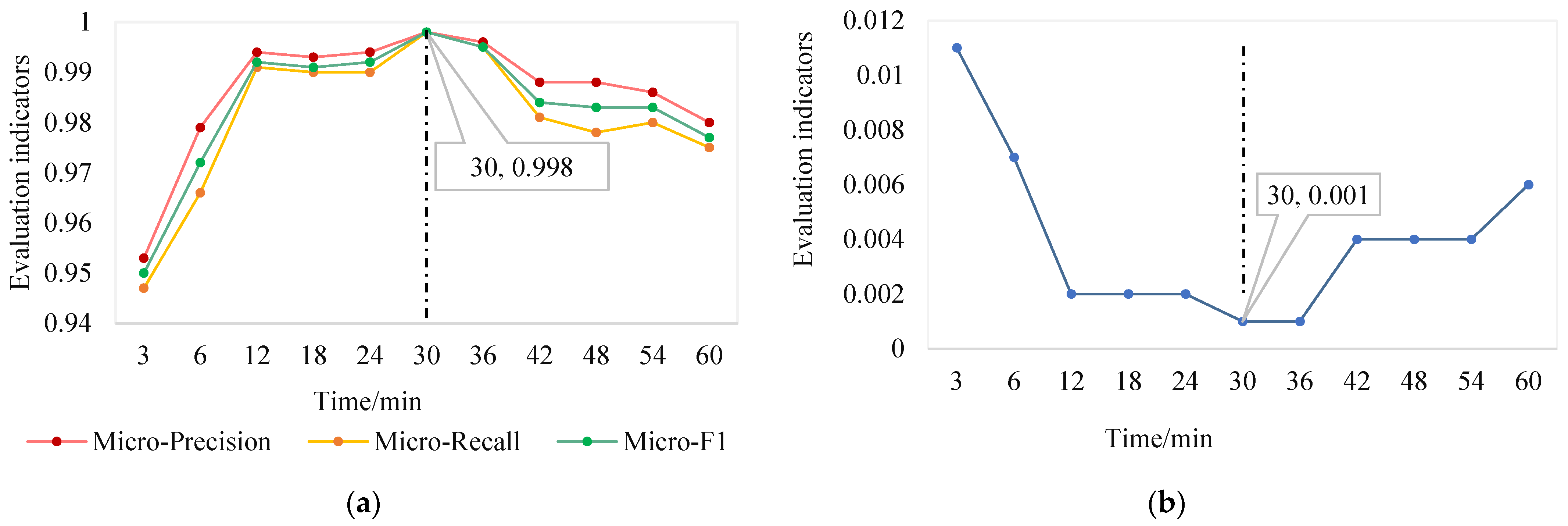
4.1. Experimental Configuration and Evaluation Indicators

The experimental environment for model training is Python 3.8.12 and TensorFlow 2.7.0. Through experimental verification, it has been found that the vector representation of entity and relationship sets in the TransR model works best when the length is 4; exceeding 4 may lead to overfitting. The number of module iterations in the transformer model is six, and each multi-head attention mechanism contains four self-attention mechanisms. The activation function in the fully connected layer is Relu, and the activation function in the output layer is Sigmoid. After debugging, the other parameters of the model are shown in

Table 3. Parameter settings.

Learning Rate	Epoch	Batch Size	Sigmoid Threshold
0.0005	300	64	0.5

. The learning rate, epoch, and batch size are parameters in the model training process. Because the learning rate is too large or too small, it will affect the model’s inability to converge or slow the convergence speed. It has been experimentally verified that the best learning rate is 0.0005. Batch size and learning rate affect each other, so it is set to 64. The Sigmoid threshold is the parameter corresponding to the multi-label classification layer. Experimental verification has shown that setting the parameter to 0.5 results in a higher accuracy in identifying different types of harmonic sources.

To better evaluate the performance of the model, this article uses precision, recall, F1, and hamming loss (HL) as evaluation indicators.

• Precision focuses on the recognition of binary positive samples. The multi-label classification problem can be regarded as a multiple-binary classification problem, and the evaluation index adopts the mean micro-precision, which is the quotient of the number of correctly predicted positive samples for all categories and the number of predicted positive samples for all categories. The formula [20] is:

$$\mathrm{Micro}\text{-}\mathrm{Precision}=\frac{{\displaystyle \sum _{j=1}^p{\mathrm{TP}}_j}}{{\displaystyle \sum _{j=1}^p{\mathrm{TP}}_j+{\displaystyle \sum _{j=1}^p{\mathrm{FP}}_j}}},$$

(6)

where TP represents the number of positive samples identified as positive samples, and FP represents the number of negative samples identified as positive samples. p represents the number of labels for each sample, consistent with the number of harmonic sources, and j represents a type of harmonic source. The larger the result, the higher the accuracy of the prediction and the better the recognition effect.

2.

Recall represents the coverage of binary positive sample prediction, and the multi-label classification metric is micro-recall. The formula [20] is:

$$\mathrm{Micro}\text{-}\mathrm{Recall}=\frac{{\displaystyle \sum _{j=1}^p{\mathrm{TP}}_j}}{{\displaystyle \sum _{j=1}^p{\mathrm{TP}}_j+{\displaystyle \sum _{j=1}^p{\mathrm{FN}}_j}}},$$

(7)

where FN represents the number of positive samples incorrectly identified as negative samples. A high recall rate indicates that the model has good coverage of positive samples, while a low recall rate declares that the model has missed some positive samples.

3.

F1 considers both accuracy and recall, which better represent the effectiveness of classification. In the multi-label classification problem, micro-F1 is used to represent, and the formula [20] is:

$$\mathrm{Micro}\text{-}\mathrm{F}1=2\times \frac{\mathrm{Micro}\text{-}\mathrm{Recall}\times \mathrm{Micro}\text{-}\mathrm{Precision}}{\mathrm{Micro}\text{-}\mathrm{Recall}+\mathrm{Micro}\text{-}\mathrm{Precision}},$$

(8)

4.

HL focuses on predicting incorrect labels, that is, directly comparing the predicted tags with the authentic labels bit by bit and calculating the quotient of the number of predicted error labels and the total number of marks. HL ranges from 0 to 1, with smaller HL indicating better prediction performance. An HL of 0 indicates that the prediction is right, while, conversely, it declares all errors. The formula [20] is:

$$\mathrm{HL}=\frac{{\displaystyle \sum _{k=1}^n{\displaystyle \sum _{j=1}^p(y_k^j\ne {\widehat{y}}_k^j)}}}{p\times n},$$

(9)

where $y_k^j$ is the authentic label of the authentic specimen x_k, the other is the predicted label, n is the number of samples, and the denominator represents the total number of labels. The consistency of each tag for each sample is compared in sequence and the total number of predicted wrong marks is calculated, including missed and false labels.

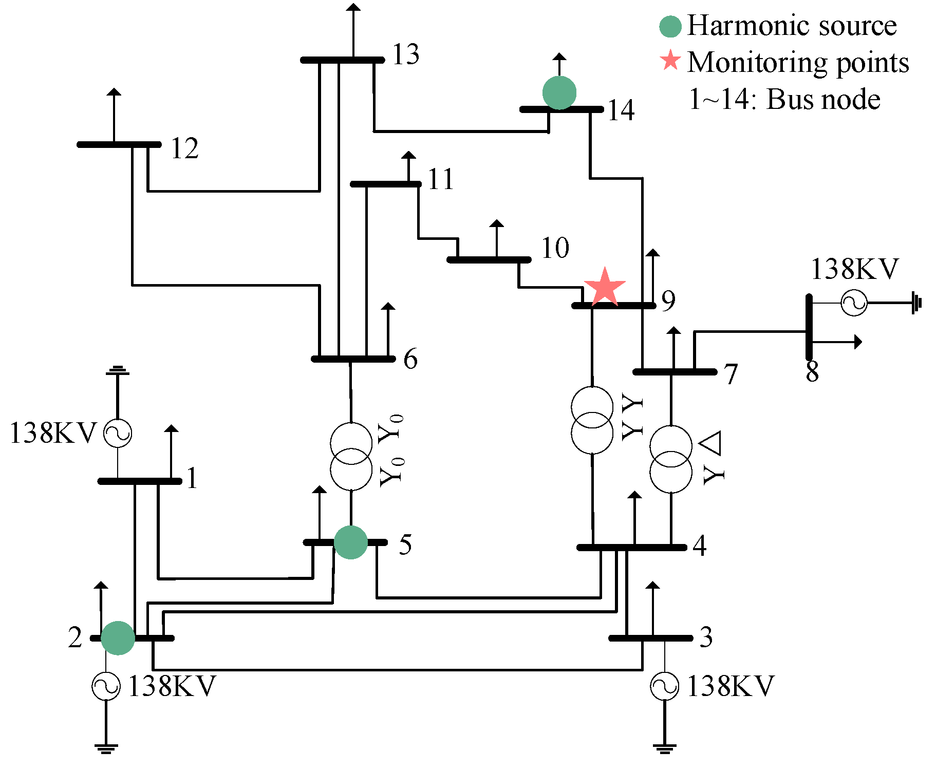
4.2. Example Analysis of Measured Data

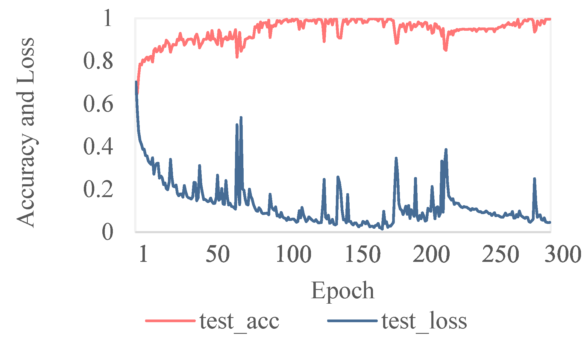
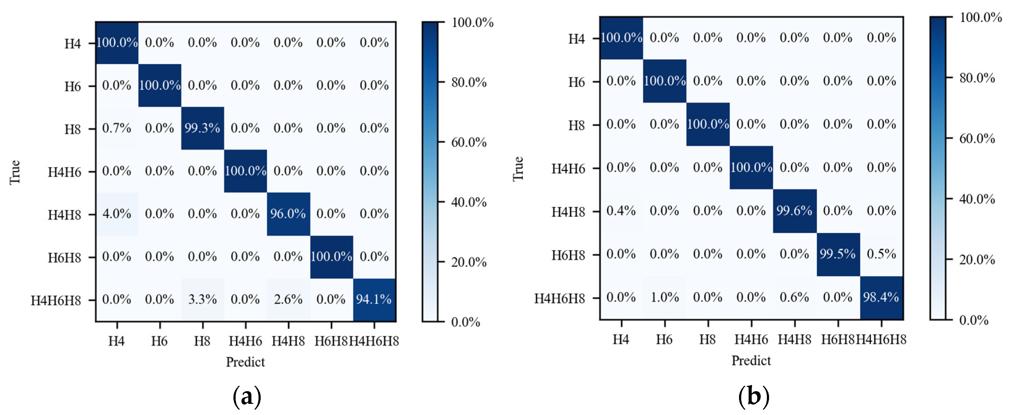
This paper uses the measured harmonic data of the power grid in a certain area to identify multiple harmonic sources, including eight harmonic sources such as electric vehicle charging stations, electric heating loads, electrified railways, wind farms, photovoltaics, rail transit, converter transformer side, and rolling mills. The time interval of the harmonic current data is 3 min, that is, a total of 480 sample points per day. This article selects 85 days of sampling data starting from 1 March 2021. Each type of harmonic source has 40,800 pieces of harmonic current data, totaling 326,400 harmonic sample data. Multiple comparative experiments are designed to verify the impact of time series on harmonic source identification and determine the optimal time scale. The sliding step size is set to 1, and then the input sample set for the model is sequentially constructed.

Figure 8 shows the experimental results for eight factual harmonic source data. The four evaluation indicators have the worst performance when the time is 5 min, which only includes individual frequency domain data. As time increases, the classification effect significantly improves, but the fluctuation is not significant until it reaches its peak at 30 min. Continuing to increase the time step, the classification effect gradually deteriorates. The experiment not only verifies that 30 min is the optimal time scale but also demonstrates that time-frequency analysis has a more significant classification effect than frequency-domain analysis alone.

Table 4. Comparison of time-frequency and frequency-domain identification results.

Harmonic	Micro-Precision		Micro-Recall		Micro-F1		HL
	Time-Frequency	Frequency	Time-Frequency	Frequency	Time-Frequency	Frequency	Time-Frequency	Frequency
H1	0.996	0.999	0.999	0.899	0.997	0.946	0.002	0.021
H2	1.000	1.000	1.000	1.000	1.000	1.000	0.000	0.000
H3	0.992	0.967	0.998	0.986	0.995	0.976	0.001	0.003
H4	1.000	0.998	1.000	0.982	1.000	0.990	0.000	0.004
H5	1.000	0.985	0.998	0.889	0.999	0.935	0.001	0.023
H6	0.997	0.982	1.000	1.000	0.998	0.991	0.000	0.000
H7	0.999	0.898	0.989	0.971	0.994	0.933	0.003	0.006
H8	1.000	0.997	1.000	1.000	1.000	0.998	0.000	0.000
Avg	0.998	0.978	0.998	0.966	0.998	0.971	0.001	0.007

shows the evaluation indicators on the test set based on individual frequency-domain features and comparative experiments based on both time-frequency features, including the recognition results and average values for each class. The results show that among the eight types of harmonic source data, except for the relatively low precision index of harmonic data in H₁, the evaluation indicators based on time-frequency feature analysis are mostly superior to the individual frequency-domain analysis indicators. Time-frequency analysis can better identify the harmonic characteristics of different harmonic sources and improve identification accuracy.

5. Simulation

The above experiment identifies single harmonic source data in real situations. Due to the unknown type of composite harmonic source in real data, manual annotation is time-consuming, laborious, and prone to errors. Therefore, combining factual data with simulation software, simulating the composite situation of ground truth, and obtaining the simulated composite harmonic source data (based on these data) further validate the effectiveness and feasibility of the model.

This article builds an IEEE14 node standard distribution network on a simulation platform and sequentially injects different types of single harmonic sources into the network. Composite harmonic data are collected from monitoring points. The injected data are real monitoring data, and odd harmonic currents within 25 for each harmonic source are injected according to the time series, retaining the frequency-domain characteristics and time fluctuation trends of different harmonic sources. To better match the situation where the distance between harmonic sources in the power grid is relatively large, three harmonic source data (H₄, H₆, and H₈) from the above eight sources are selected for composite simulation as examples. To prevent mutual influence between harmonic sources, H₄ harmonics are not injected into the network when collecting composite data of H₆ and H₈, and the same applies to other situations. Figure 9 shows a distribution network where three types of harmonic sources coexist. Simulated harmonics of H₄, H₆, and H₈ are added to busbars 2, 5, and 14 in sequence, and monitoring points are set up on busbar 9. A total of seven harmonic current data are collected, including H₄, H₆, H₈, H₄H₆, H₄H₈, H₆H₈, and H₄H₆H₈. A total of 3360 data samples are simulated for each scenario, totaling 23520.

Figure 10 shows the fluctuation of accuracy and loss values during the testing process of the TTM model. As epoch increases, the overall loss value continuously decreases and eventually stabilizes. The accuracy increases with the increase in epoch, gradually approaching 100%, and finally reaching the effect of model convergence. The experimental results show that the trained model can accurately identify any single or composite harmonic source data without knowing the number or type of composite harmonic sources. The recognition accuracy of the TTM model can reach over 99%.

Two comparative experiments are designed to verify the effectiveness of knowledge representation in classification models. Figure 11 shows the classification and recognition results of seven types of simulated data during the testing process. Figure 11a shows the results of multi-label recognition based on the transformer model. Only 0.7% of H₈ harmonic data are identified as H₄ harmonic data. The recognition performance of a compound harmonic source is significantly lower than that of a single harmonic source. Among them, 4% of H₄H₈ compound harmonic sources are recognized as H₄ harmonic sources, and 5.9% of H₄H₆H₈ compound harmonic sources are identified as H₄ and H₄H₈. Figure 11b shows the harmonic source identification results of the TTM model. Experimental results have shown that by integrating TransR knowledge representation based on the transformer multi-label classification model, semantic information is transformed into a vector representation, which increases the internal cohesion of harmonic current data, reduces the coupling degree between different harmonic current data, improves the recognition accuracy of composite harmonic sources, and achieves almost 100% accurate recognition. Only 0.4% of H₄H₈ and 0.5% of H₆H₈, and 1.6% of H₄H₆H₈ recognition errors, and all other accuracies are 100%.

6. Discussion

Basic machine learning models that are used to identify harmonic sources have relatively low recognition accuracy. Reference [25] introduces two methods based on support vector machine (SVM) and naive Bayes (NB) classifiers to classify the voltage and current characteristics observed on different PCCs. When the simulation testing system is small, SVM shows better performance. However, it can only recognize predefined combinations of general loads connected to PCCs. Reference [26] conducted harmonic source identification for different loads such as fluorescent lamps, televisions, fans, etc. This study utilizes the radial basis function neural network (RBFNN). RBFNN is more accurate and efficient than SVM due to lower computational requirements and better feature selection. However, the RBF neural network needs to adjust many parameters, such as the number, center position, and width of radial basis functions. In practice, finding the optimal parameter configuration can take a lot of time and computational resources.

While artificial-intelligence-based classification has made significant progress in various fields such as image processing, there is still room for improvement in harmonic source classification. This paper explores the application of neural networks such as LSTM, convolutional neural network (CNN), and the transformer model, all of which are widely used for classification and recognition, in the identification of composite harmonic sources. These models are compared with TTM models for analysis. As shown in

Table 5. Recognition results of different classification models.

Classfication Model	Evaluating Indicator
	Micro-Precision	Micro-Recall	Micro-F1	HL
LSTM + Attention [27]	0.918	0.913	0.906	0.051
LSTM + CNN [28]	0.940	0.927	0.925	0.047
Transformer [29]	0.985	0.985	0.985	0.007
TTM	0.996	0.996	0.996	0.001

, for the seven simulated harmonic current data, LSTM exhibits the worst performance, while CNN outperforms the attention mechanism. The transformer model demonstrates better recognition, with the TTM model showing the best identification performance for composite harmonic sources. The fusion of TransR knowledge representation effectively enhances the stability, convergence speed, and recognition accuracy of the original transformer model, thereby improving the overall generalization ability and robustness of the model. Furthermore, the TTM model, grounded in artificial intelligence methods, achieves autonomous feature extraction, thus avoiding the issues of information loss or insufficient extraction commonly associated with traditional harmonic source recognition methods that rely on physical mechanisms for data feature extraction.

The fusion of TransR knowledge representation proves effective in enhancing the stability, convergence speed, and recognition accuracy of the original transformer model. This fusion further augments the overall generalization ability and robustness of the model. The TTM model, grounded in artificial intelligence methods, achieves autonomous feature extraction, circumventing issues of information loss or insufficient extraction associated with traditional harmonic source recognition methods that rely on physical mechanisms for data feature extraction.

7. Conclusions

Under the emerging power system, the interconnection of harmonic sources from multiple origins and various transformations is becoming more prevalent. The amalgamation of these harmonic sources is intricate, leading to a growing concern regarding harmonic pollution. This issue significantly impacts power quality and consumer electricity consumption. Traditional models for identifying harmonic sources predominantly rely on physical models and remain limited in handling single harmonic source identification. To address this gap, this paper introduces a novel composite harmonic source identification method that leverages the fusion of knowledge representation and transformer architecture, focusing on the time-frequency characteristics of harmonic data. The innovations presented in this article are primarily evident in the following areas:

• TTM model integrating time-frequency feature extraction.

Traditional methods for addressing harmonic source identification problems often focus on a single type of harmonic source or employ only one feature extraction method, such as solely utilizing time-domain features or frequency-domain features. Recognizing the challenges posed by the difficulty in separating source current data and incomplete feature extraction, this paper proposes a TTM harmonic source identification network model. This innovative approach starts with the following two dimensions: the time domain and the frequency domain. Its goal is to decouple composite harmonic sources and accurately identify different types of harmonic sources.

The model achieves this by first extracting discrete semantic features from harmonic data. These features are then converted into representation vectors with semantic information using TransR. This process increases the feature differences between composite harmonic data and reduces the coupling degree between different harmonic source data. Combining TransR with the transformer model allows for normative constraints on the self-attention mechanism, providing enhanced learning and reasoning capabilities. The model outputs the type of each harmonic source datum along with corresponding triplet semantic features, thereby increasing interpretability. This innovation significantly improves identification accuracy and offers an effective solution for accurately identifying complex harmonic sources in power systems.

2.

Feasibility verification applied to actual scenarios.

In the traditional method, the unknown parameters of the harmonic network and the asynchronous data of each monitoring point limit the accuracy of harmonic source identification. The TTM model learns data characteristics through neural networks and does not need to know the specific parameters of the system in advance. It avoids some difficulties and limitations in traditional methods and solves the problem of unknown harmonic network parameters and unsynchronized data at each monitoring point. In addition, the training data of the TTM model contain a large amount of harmonic current data collected by power system monitoring devices. These data are collected in real-time during actual power system operation, so they are authentic and representative. This study applies the proposed composite harmonic source identification method to actual harmonic data collected by power system monitoring devices and conducts full verification and experiments. Experimental results show that this method achieves high recognition accuracy on both real and simulated data and achieves good recognition results even on untrained composite harmonic source data. The TTM model shows high generalization ability in experiments, which provides reliable support for the model to face variable and unknown power system conditions in practical applications.

References

1. Sun, Y.Y.; Li, S.R.; Shi, F. Division of responsibilities for multiple harmonic sources in distribution networks containing distributed harmonic sources. Proc. CSEE 2019, 39, 5389–5398. [Google Scholar]
2. Shao, Z.G.; Xu, H.B.; Xiao, S.Y. Harmonic problems in new energy grids. Power Syst. Prot. Control 2021, 49, 178–187. [Google Scholar]
3. Ding, T.; Chen, H.K.; Wu, B. Overview of methods for locating multiple harmonic sources and quantifying harmonic responsibilities. Electr. Power Autom. Equip. 2020, 40, 19–30. [Google Scholar]
4. Farhoodnea, M.; Mohamed, A.; Shareef, H. A new method for determining multiple harmonic source locations in a power distribution system. In Proceedings of the IEEE International Conference on Power and Energy, Kuala Lumpur, Malaysia, 29 November–1 December 2010. [Google Scholar]
5. Xu, F.; Yang, H.; Zhao, J. Study on constraints for harmonic source determination using active power direction. IEEE Trans. Power Deliv. 2018, 33, 2683–2692. [Google Scholar] [CrossRef]
6. Wang, B.; Ma, G.; Xiong, J. Several sufficient conditions for harmonic source identification in power systems. IEEE Trans. Power Deliv. 2018, 33, 3105–3113. [Google Scholar] [CrossRef]
7. Huang, C.; Lin, C. Multiple harmonic source classification using a self-organization feature map network with voltage current wavelet transformation patterns. Appl. Math. Model. 2015, 39, 5849–5861. [Google Scholar] [CrossRef]
8. Jopri, M.; Abdullah, A.; Karim, R. Accurate harmonic source identification using S transform. Telecommun. Comput. Electron. Control 2020, 18, 2708–2717. [Google Scholar] [CrossRef]
9. Karimzadeh, F.; Esmaeili, S.; Hosseinian, S.H. A Novel method for noninvasive estimation of utility harmonic impedance based on complex independent component analysis. IEEE Trans. Power Deliv. 2015, 30, 1843–1852. [Google Scholar] [CrossRef]
10. Gao, P.; Tian, M.; Wang, L. Harmonic source identification method based on sinusoidal approximation. J. Phys. Conf. Ser. 2022, 2290, 012054. [Google Scholar] [CrossRef]
11. Zhang, Y.; Ruan, Z.X.; Shao, Z.G. Division of responsibilities for multi harmonic sources for distributed power grid connection. Proc. CSU—EPSA 2022, 34, 56–64. [Google Scholar]
12. Eslami, A.; Negnevitsky, M.; Franklin, E. Review of AI applications in harmonic analysis in power systems. Renew. Sustain. Energy Rev. 2022, 154, 1–26. [Google Scholar] [CrossRef]
13. Anggriawan, D.O.; Wahjono, E.; Sudiharto, I. Identification of short duration voltage variations based on short time fourier transform and artificial neural network. In Proceedings of the International Electronics Symposium, Surabata, Indonesia, 29–30 September 2020. [Google Scholar]
14. Ge, X.L.; Liu, Y.W. A dynamic parameter model of harmonic source networks. IEEE Trans. Power Deliv. 2020, 35, 1093–1101. [Google Scholar] [CrossRef]
15. Li, Q. Research on Harmonic Source Identification Method Based on Harmonic Monitoring Data. Master’s Thesis, Northern University of Technology, Beijing, China, 2020. [Google Scholar]
16. Available online: https://arxiv.org/abs/1706.03762 (accessed on 8 January 2024).
17. Xu, S.; Liu, Z.Y.; Li, Y.C. Research on intelligent detection methods for false data injection attacks in battery energy storage systems. Proc. CSEE 2023, 43, 6628–6639. [Google Scholar]
18. Gao, F.J.; Wang, H.Y.; Dang, R. Interpretability analysis and model update research of transformer based transient stability assessment mode. Power Syst. Prot. Control 2023, 51, 15–25. [Google Scholar]
19. Ruan, C.; Qi, L.H.; Wang, H. Demand response intelligent recommendation combining knowledge graph and neural tensor network. Power Syst. Technol. 2021, 45, 2131–2140. [Google Scholar]
20. Liang, Y.; Li, K.J.; Ma, Z. Multilabel classification model for type recognition of single-phase-to-ground fault based on KNN-Bayesian method. IEEE Trans. Ind. Appl. 2021, 57, 1294–1302. [Google Scholar] [CrossRef]
21. Jin, G.; Zhu, Q.Z.; Meng, Y. Multilabel classification algorithm for power quality disturbances based on multi-layer limit learning machines. Power Syst. Prot. Control 2020, 48, 96–105. [Google Scholar]
22. Qu, T.; Ren, Y.; Lin, H.X.; Du, D.L.; Chen, B.X.; Li, P.Z.; Lv, R.Y. Power Supply Quality—Harmonics in Public Power Supply Networks; China Standard Press: Beijing, China, 1994; pp. 1–8. [Google Scholar]
23. Zhang, Z.; Jia, J.; Wan, Y. TransR*: Representation learning model by flexible translation and relation matrix projection. J. Intell. Fuzzy Syst. 2021, 40, 1–9. [Google Scholar] [CrossRef]
24. Wu, D.; Zhao, J.; Li, M. A knowledge representation method for multiple pattern embeddings based on entity-relation mapping matrix. In Proceedings of the International Joint Conference on Neural Networks (IJCNN), Padua, Italy, 18–23 July 2022. [Google Scholar]
25. Jopri, M.H.; Ab Ghani, M.R.; Abdullah, A.R.; Manap, M.; Sutikno, T.; Too, J. K-nearest neighbor and naïve Bayes based diagnostic analytic of harmonic source identification. Bull. Electr. Eng. Inform. 2020, 9, 2650–2657. [Google Scholar] [CrossRef]
26. Mubarok, A.F.; Octavira, T.; Sudiharto, I.; Wahjono, E.; Anggriawan, D.O. Identification of harmonic loads using fast fourier transform and radial basis Function Neural Network. In Proceedings of the 2017 International Electronics Symposium on Engineering Technology and Applications (IES-ETA), Surabaya, Indonesia, 26–27 September 2017. [Google Scholar]
27. Zhao, Z.; Lv, N.; Xiao, R. A novel penetration state recognition method based on lstm with auditory attention during pulsed GTAW. IEEE Trans. Ind. Inform. 2023, 19, 9565–9575. [Google Scholar] [CrossRef]
28. Nguyen, C.; Hoang, T.M.; Cheema, A.A. Channel estimation using CNN-LSTM in RIS-NOMA assisted 6G network. IEEE Trans. Mach. Learn. Commun. Netw. 2023, 1, 43–60. [Google Scholar] [CrossRef]
29. Saha, T.; Ramesh, S.J.; Saha, S. BERT-Caps: A transformer-based capsule network for tweet act classification. IEEE Trans. Comput. Soc. Syst. 2020, 7, 1168–1179. [Google Scholar] [CrossRef]
Figure 1. Characteristics of harmonic current data at a certain moment.
Electronics 13 01275 g001
Figure 2. Frequency domain characteristics of composite harmonic sources. (a) Harmonic data for H6 and H8 coupling; (b) harmonic data for H4, H6 and H8 coupling.
Electronics 13 01275 g002
Figure 3. Time domain characteristics of composite harmonic sources. (a) Harmonic data for H1; (b) harmonic data for H2; (c) harmonic data for H3; (d) harmonic data for H4; (e) harmonic data for H5; (f) harmonic data for H6; (g) harmonic data for H7; (h) harmonic data for H8.
Electronics 13 01275 g003
Figure 4. Harmonic source characteristic triplet.
Electronics 13 01275 g004
Figure 5. TransR knowledge representation.
Electronics 13 01275 g005
Figure 6. Architecture diagram of TTM harmonic source identification model.
Electronics 13 01275 g006
Figure 7. Transformer module.
Electronics 13 01275 g007
Figure 8. Change trends of four evaluation indicators at different time scales. (a) Change trends of micro-precision, micro-recall, and micro-F1 at different time scales; (b) change trends of HL at different time scales.
Electronics 13 01275 g008
Figure 9. Simulation circuit diagram.
Electronics 13 01275 g009
Figure 10. Iterative process of TTM.
Electronics 13 01275 g010
Figure 11. Comparison of model accuracy under different noises. (a) Results of the transformer model; (b) results of the TTM model.
Electronics 13 01275 g011