
Energy Efficient Wireless Signal Detection: A Revisit through the Lens of Approximate Computing


Abstract
:1. Introduction
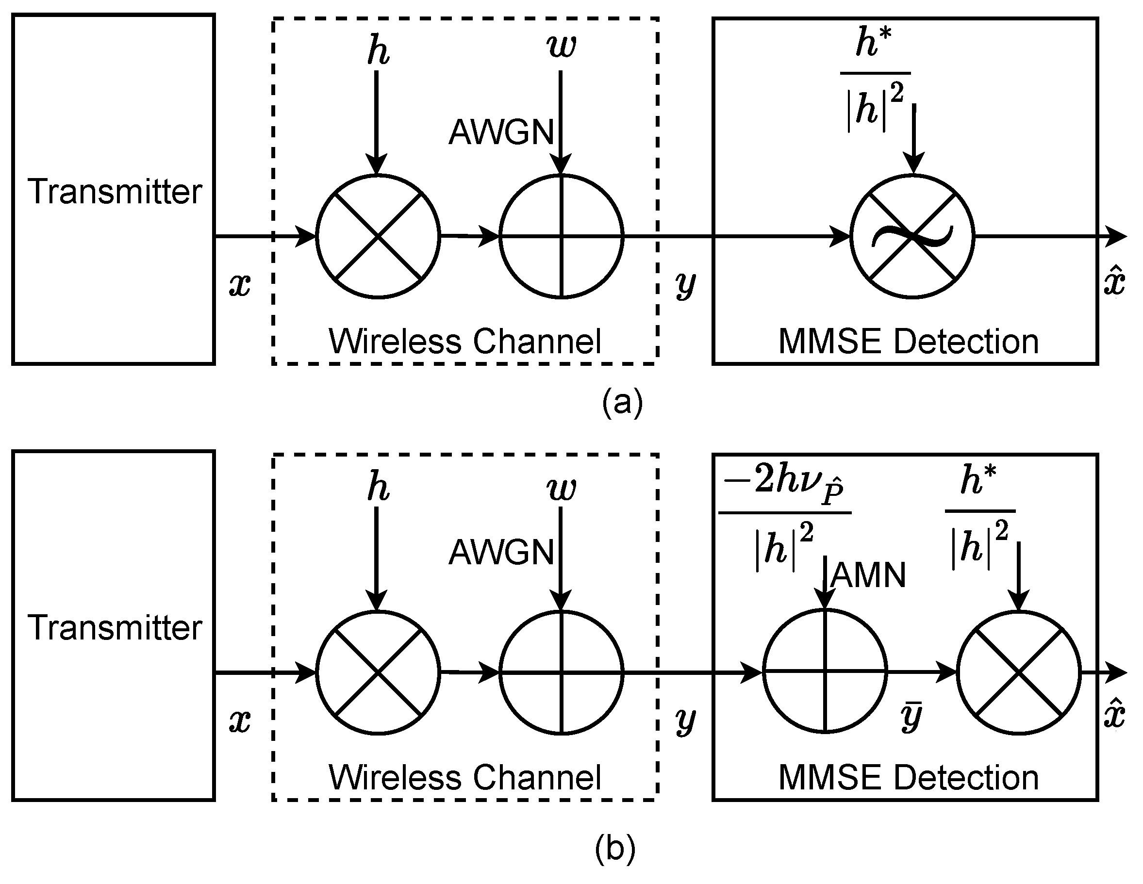
- Modeling of a constant noise model for wireless signal detection to evaluate the impact of irregularities caused by approximate multiplication. AMN is a novel constant noise model that effectively captures irregularities of TM for QPSK MMSE signal detection.
- Gauging the effect of TM on Symbol Error Rate (SER) of QPSK MMSE signal detection. The derived analytical expression computes SER by using AMN.
- Proposition of resiliency metrics to provide insights into resilient TM configurations for QPSK MMSE signal detection. A TM configuration characterized by a low level of approximation proves advantageous in high SNR regimes, whereas one with a high level of approximation is preferable in low SNR regimes.
2. Related Work
3. Methodology
3.1. Preliminary
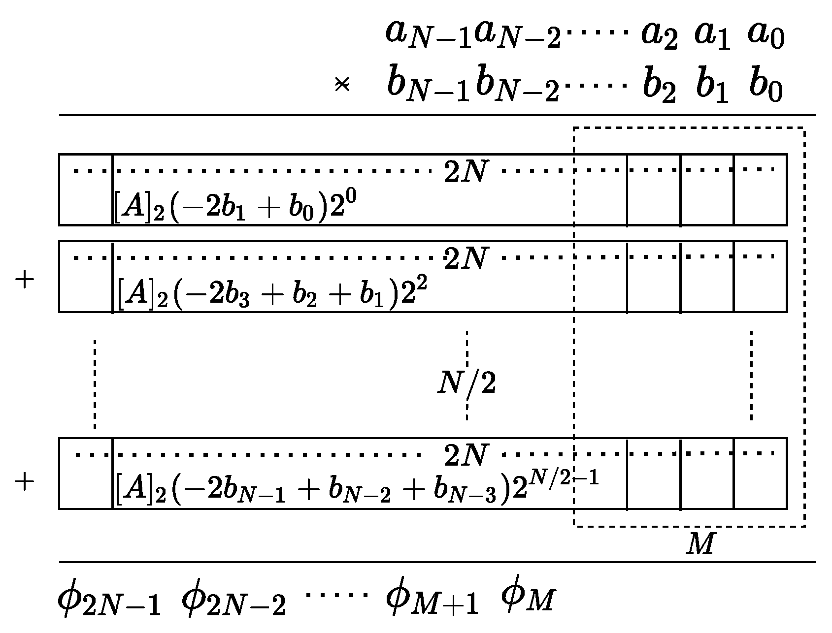
3.2. Truncated Multiplication
| Algorithm 1 Signed multiplication using Radix-4 Booth algorithm. |
|
3.2.1. Regression Estimate for
3.2.2. Energy Efficiency
3.3. SER Expression
3.3.1. AMN Model
3.3.2. SER Evaluation Using AMN
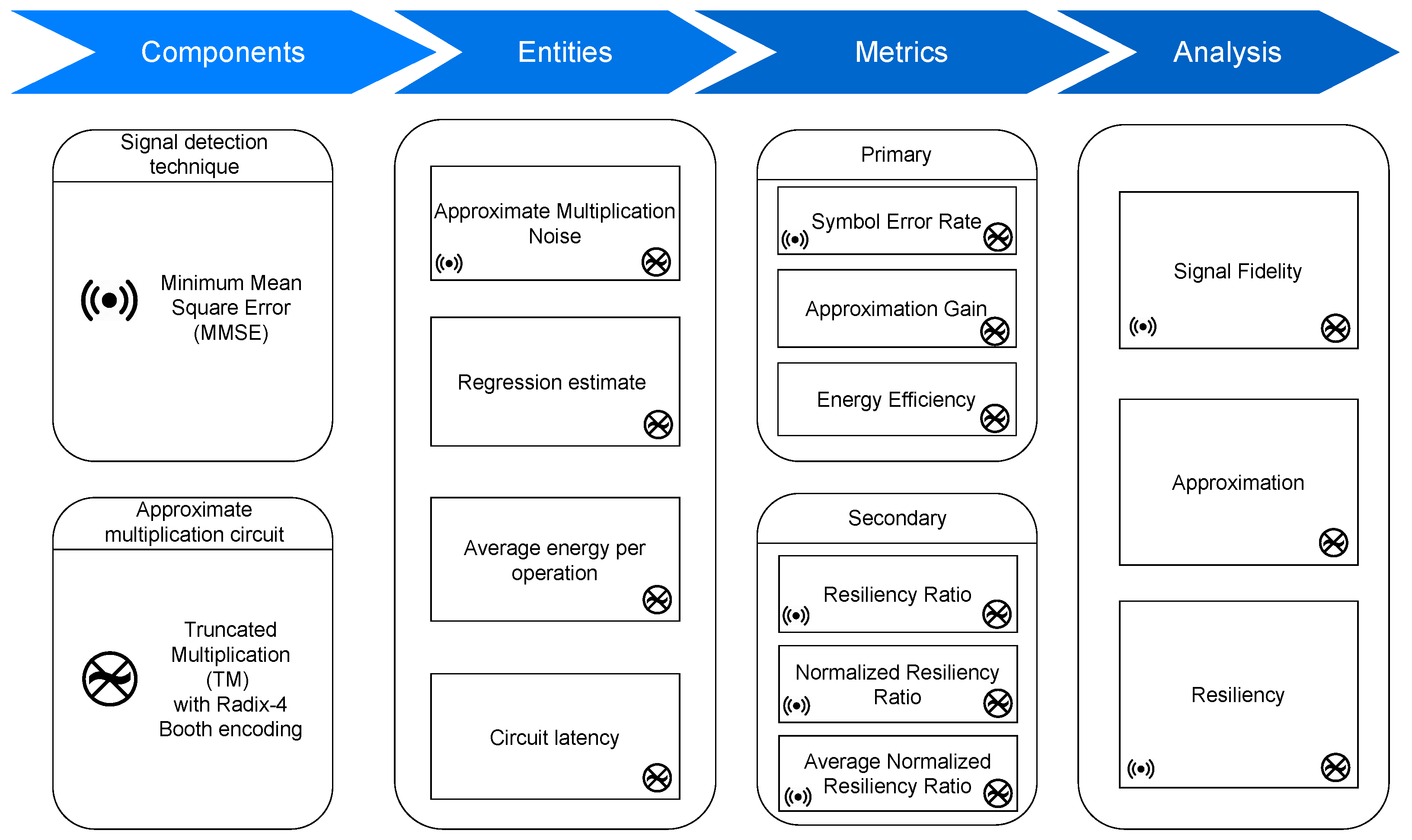
4. Analysis
4.1. Signal Fidelity Analysis
4.2. Approximation Analysis
4.3. Resiliency Analysis
5. Conclusions
Author Contributions
Funding
Data Availability Statement
Conflicts of Interest
References
- Jiang, W.; Han, B.; Habibi, M.A.; Schotten, H.D. The Road Towards 6G: A Comprehensive Survey. IEEE Open J. Commun. Soc. 2021, 2, 334–366. [Google Scholar] [CrossRef]
- Chowdhury, M.Z.; Shahjalal, M.; Ahmed, S.; Jang, Y.M. 6G Wireless Communication Systems: Applications, Requirements, Technologies, Challenges, and Research Directions. IEEE Open J. Commun. Soc. 2020, 1, 957–975. [Google Scholar] [CrossRef]
- Rajatheva, N.; Atzeni, I.; Bjornson, E.; Bourdoux, A.; Buzzi, S.; Dore, J.B.; Erkucuk, S.; Fuentes, M.; Guan, K.; Hu, Y.; et al. White paper on broadband connectivity in 6G. arXiv 2020, arXiv:2004.14247. [Google Scholar]
- Andersson, C.; Bengtsson, J.; Byström, G.; Frenger, P.; Jading, Y.; Nordenström, M. Improving energy performance in 5G networks and beyond. Ericsson Technol. Rev. 2022, 2022, 2–11. [Google Scholar] [CrossRef]
- Viswanathan, H.; Mogensen, P.E. Communications in the 6G era. IEEE Access 2020, 8, 57063–57074. [Google Scholar] [CrossRef]
- López-Pérez, D.; De Domenico, A.; Piovesan, N.; Xinli, G.; Bao, H.; Qitao, S.; Debbah, M. A survey on 5G radio access network energy efficiency: Massive MIMO, lean carrier design, sleep modes, and machine learning. IEEE Commun. Surv. Tutor. 2022, 24, 653–697. [Google Scholar] [CrossRef]
- Chih-Lin, I.; Han, S.; Bian, S. Energy-efficient 5G for a greener future. Nat. Electron. 2020, 3, 182–184. [Google Scholar]
- Seskar, I.; Patwary, M.; Dutta, A.; Chaparadza, R.; Elkotab, M. INGR Roadmap. In Proceedings of the 2022 IEEE Future Networks World Forum (FNWF), Montreal, QC, Canada, 10–14 October 2022; pp. 1–38. [Google Scholar] [CrossRef]
- Cheng, X.; Hu, Y.; Varga, L. 5G network deployment and the associated energy consumption in the UK: A complex systems’ exploration. Technol. Forecast. Soc. Chang. 2022, 180, 121672. [Google Scholar] [CrossRef]
- Khalili, R.; Salamatian, K. A new analytic approach to evaluation of packet error rate in wireless networks. In Proceedings of the 3rd Annual Communication Networks and Services Research Conference (CNSR’05), Halifax, NS, Canada, 16–18 May 2005; pp. 333–338. [Google Scholar]
- Sodhro, A.H.; Obaidat, M.S.; Abbasi, Q.H.; Pace, P.; Pirbhulal, S.; Fortino, G.; Imran, M.A.; Qaraqe, M. Quality of service optimization in an IoT-driven intelligent transportation system. IEEE Wirel. Commun. 2019, 26, 10–17. [Google Scholar] [CrossRef]
- Pundir, M.; Sandhu, J.K. A systematic review of quality of service in wireless sensor networks using machine learning: Recent trend and future vision. J. Netw. Comput. Appl. 2021, 188, 103084. [Google Scholar] [CrossRef]
- Beshley, H.; Beshley, M.; Medvetskyi, M.; Pyrih, J. QoS-aware optimal radio resource allocation method for machine-type communications in 5G LTE and beyond cellular networks. Wirel. Commun. Mob. Comput. 2021, 2021, 9966366. [Google Scholar] [CrossRef]
- Bertin, E.; Crespi, N.; Magedanz, T. Shaping Future 6G Networks: Needs, Impacts, and Technologies; John Wiley & Sons: Hoboken, NJ, USA, 2021. [Google Scholar]
- Chochliouros, I.P.; Kourtis, M.A.; Spiliopoulou, A.S.; Lazaridis, P.; Zaharis, Z.; Zarakovitis, C.; Kourtis, A. Energy efficiency concerns and trends in future 5G network infrastructures. Energies 2021, 14, 5392. [Google Scholar] [CrossRef]
- He, S.; Zhang, Y.; Wang, J.; Zhang, J.; Ren, J.; Zhang, Y.; Zhuang, W.; Shen, X. A survey of millimeter-wave communication: Physical-layer technology specifications and enabling transmission technologies. Proc. IEEE 2021, 109, 1666–1705. [Google Scholar] [CrossRef]
- Wang, Z.; Du, Y.; Wei, K.; Han, K.; Xu, X.; Wei, G.; Tong, W.; Zhu, P.; Ma, J.; Wang, J.; et al. Vision, application scenarios, and key technology trends for 6G mobile communications. Sci. China Inf. Sci. 2022, 65, 151301. [Google Scholar] [CrossRef]
- Leon, V.; Hanif, M.A.; Armeniakos, G.; Jiao, X.; Shafique, M.; Pekmestzi, K.; Soudris, D. Approximate Computing Survey, Part II: Application-Specific & Architectural Approximation Techniques and Applications. arXiv 2023, arXiv:2307.11128. [Google Scholar]
- Mittal, S. A Survey of Techniques for Approximate Computing. ACM Comput. Surv. 2016, 48, 62. [Google Scholar] [CrossRef]
- Que, H.H.; Jin, Y.; Wang, T.; Liu, M.K.; Yang, X.H.; Qiao, F. A Survey of Approximate Computing: From Arithmetic Units Design to High-Level Applications. J. Comput. Sci. Technol. 2023, 38, 251–272. [Google Scholar] [CrossRef]
- Liu, W.; Lombardi, F. Approximate Computing; Springer: Berlin/Heidelberg, Germany, 2022. [Google Scholar]
- Bosio, A.; Ménard, D.; Sentieys, O. Approximate Computing Techniques: From Component-to Application-Level; Springer International Publishing: Cham, Switzerland, 2022. [Google Scholar]
- Zamani, A.R.; Petri, I.; Diaz-Montes, J.; Rana, O.; Parashar, M. Edge-supported approximate analysis for long running computations. In Proceedings of the 2017 IEEE 5th International Conference on Future Internet of Things and Cloud (FiCloud), Prague, Czech Republic, 21–23 August 2017; pp. 321–328. [Google Scholar]
- Traiola, M.; Savino, A.; Di Carlo, S. Probabilistic estimation of the application-level impact of precision scaling in approximate computing applications. Microelectron. Reliab. 2019, 102, 113309. [Google Scholar] [CrossRef]
- Damsgaard, H.J.; Ometov, A.; Nurmi, J. Approximation Opportunities in Edge Computing Hardware: A Systematic Literature Review. ACM Comput. Surv. 2023, 55, 1–49. [Google Scholar] [CrossRef]
- Damsgaard, H.J.; Ometov, A.; Mowla, M.M.; Flizikowski, A.; Nurmi, J. Approximate computing in B5G and 6G wireless systems: A survey and future outlook. Comput. Netw. 2023, 233, 109872. [Google Scholar] [CrossRef]
- Zhou, Y.; Chen, Z.; Lin, J.; Wang, Z. A high-speed successive-cancellation decoder for polar codes using approximate computing. IEEE Trans. Circuits Syst. II Express Briefs 2018, 66, 227–231. [Google Scholar] [CrossRef]
- Hao, M.; Najafi, A.; García-Ortiz, A.; Karsthof, L.; Paul, S.; Rust, J. Reliability of an industrial wireless communication system using approximate units. In Proceedings of the 2019 29th International Symposium on Power and Timing Modeling, Optimization and Simulation (PATMOS), Rhodes, Greece, 1–3 July 2019; pp. 87–90. [Google Scholar]
- Xiao, J.; Hu, J.; Han, K. Low complexity expectation propagation detection for SCMA using approximate computing. In Proceedings of the 2019 IEEE Global Communications Conference (GLOBECOM), Waikoloa, HI, USA, 9–13 December 2019; pp. 1–6. [Google Scholar]
- Idrees, M.; Maqbool, M.M.; Bhatti, M.K.; Rahman, M.M.U.; Hafiz, R.; Shafique, M. An approximate-computing empowered green 6G downlink. Phys. Commun. 2021, 49, 101444. [Google Scholar] [CrossRef]
- Ma, X.; Sun, H.; Hu, R.Q.; Qian, Y. Approximate Wireless Communication for Federated Learning. arXiv 2023, arXiv:2304.03359. [Google Scholar]
- Anghel, L.; Benabdenbi, M.; Bosio, A.; Traiola, M.; Vatajelu, E.I. Test and reliability in approximate computing. J. Electron. Test. 2018, 34, 375–387. [Google Scholar] [CrossRef]
- Wyse, M.; Baixo, A.; Moreau, T.; Zorn, B.; Sampson, A.; Bornholt, J.; Ceze, L.; Oskin, M. Mapping and Modeling Approximate Computing Techniques. Available online: https://homes.cs.washington.edu/~luisceze/approx-darpa-report.pdf (accessed on 4 December 2023).
- Bruestel, M.; Kumar, A. Accounting for systematic errors in approximate computing. In Proceedings of the Design, Automation & Test in Europe Conference & Exhibition (DATE), Lausanne, Switzerland, 27–31 March 2017; pp. 298–301. [Google Scholar]
- Scales, J.A.; Snieder, R. What is noise? Geophysics 1998, 63, 1122–1124. [Google Scholar] [CrossRef]
- Nakamura, S. A study of errors caused by impulsive noise and a simple estimation method for digital mobile communications. IEEE Trans. Veh. Technol. 1996, 45, 310–317. [Google Scholar] [CrossRef]
- Middleton, D. Non-Gaussian noise models in signal processing for telecommunications: New methods an results for class A and class B noise models. IEEE Trans. Inf. Theory 1999, 45, 1129–1149. [Google Scholar] [CrossRef]
- Shongwe, T.; Vinck, A.H.; Ferreira, H.C. A study on impulse noise and its models. SAIEE Afr. Res. J. 2015, 106, 119–131. [Google Scholar] [CrossRef]
- Rozic, N.; Banelli, P.; Begusic, D.; Radic, J. GMM-Based Symbol Error Rate Analysis for Multicarrier Systems with Impulsive Noise Suppression. IEEE Trans. Veh. Technol. 2022, 71, 13060–13076. [Google Scholar] [CrossRef]
- Abramowitz, M. Abramowitz and Stegun: Handbook of Mathematical Functions; United States Department of Commerce: Washington, DC, USA, 1972; Volume 10. [Google Scholar]
- Bewick, G.W. Fast Multiplication: Algorithms and Implementation. Ph.D. Thesis, Stanford University, Stanford, CA, USA, 1994. [Google Scholar]
- Seber, G.A.; Lee, A.J. Linear Regression Analysis; John Wiley & Sons: Hoboken, NJ, USA, 2003; Volume 330. [Google Scholar]
- Tse, D.; Viswanath, P. Fundamentals of Wireless Communication; Cambridge University Press: Cambridge, UK, 2005. [Google Scholar]
- Springer, M.D. The Algebra of Random Variables; Wiley: Hoboken, NJ, USA, 1979. [Google Scholar]
- Haykin, S. Digital Communications; Wiley: New York, NY, USA, 1988. [Google Scholar]


| Work | Description | Approximation | Modulation | QoS |
|---|---|---|---|---|
| Zhou (2018) [27] | Throughput improvement by utilizing approximate computation blocks for decoding FEC polar codes. | SC decoder. | - | FER |
| Hao (2019) [28] | Reliability assessment on utilizing approximate adders for industrial wireless communication. | FFT. | QPSK | FER |
| Xiao (2019) [29] | Complexity reduction of expectation propagation algorithm utilized for SCMA. | Variable and functional node update, log likelihood ratio computation. | - | BER |
| Idrees (2021) [30] | Gains by utilizing approximate computing units in digital signal processing filters in 6G downlink operation. | FIR filter at pulse shaping/equalization/decoding. | BPSK, QPSK, 8-PSK | BER (link), Structural Similarity Index and Correlation Coefficient (Image transmission) |
| Ma (2023) [31] | Approximate communication scheme for federated learning application. | Gradients. | QPSK, 16-QAM, 256-QAM | Test accuracy |
| = 16 † | = 20 † | |||
|---|---|---|---|---|
| 1 | ||||
| 2 | ||||
| 3 | ||||
| 4 | ||||
| 5 | ||||
| 6 | ||||
| 7 | ||||
| 8 | ||||
| 9 | - | |||
| 10 | - | |||
| 11 | - | |||
| 12 | - | |||
| 13 | - | - | ||
| 14 | - | - | ||
| 15 | - | - | ||
| 16 | - | - | ||
| 17 | - | - | - | |
| 18 | - | - | - | |
| 19 | - | - | - | |
| 20 | - | - | - | |
| Analysis | Metric | Parameter | Description |
|---|---|---|---|
| Entities | |||
| Computation | ; ; ; Operand range | As given in Table 2, values are computed by exhaustive simulation. | |
| Computation | ; ; ; Operand range:; step size = | As given in Table 2, values are computed by point estimation. | |
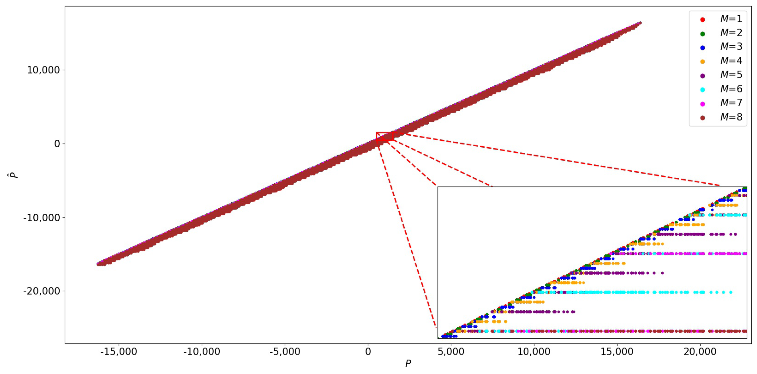
| Covariance | P, | ; ; ; Operand range | As depicted in Figure 4, P and have linear covariance. |
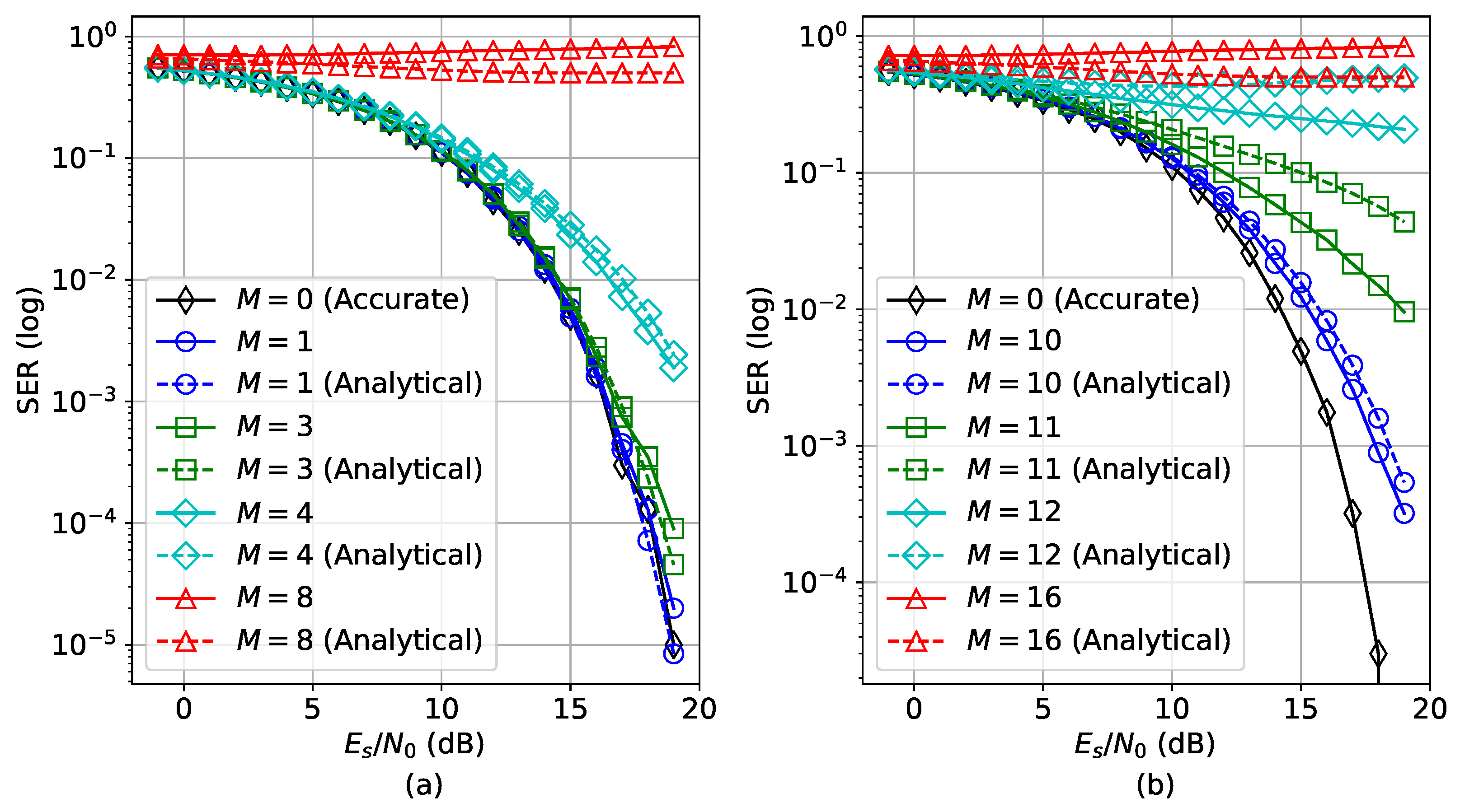
| Verification | ; ; , 5000 symbols per | As depicted in Figure 6, the analytical expression for SER tracks the SER computed by simulation. | |
| System | |||
| Signal Fidelity | ; ; ; | As depicted in Figure 7, the bound interval increases with both the SNR and channel gain, which indicates a greater degradation in SER. | |
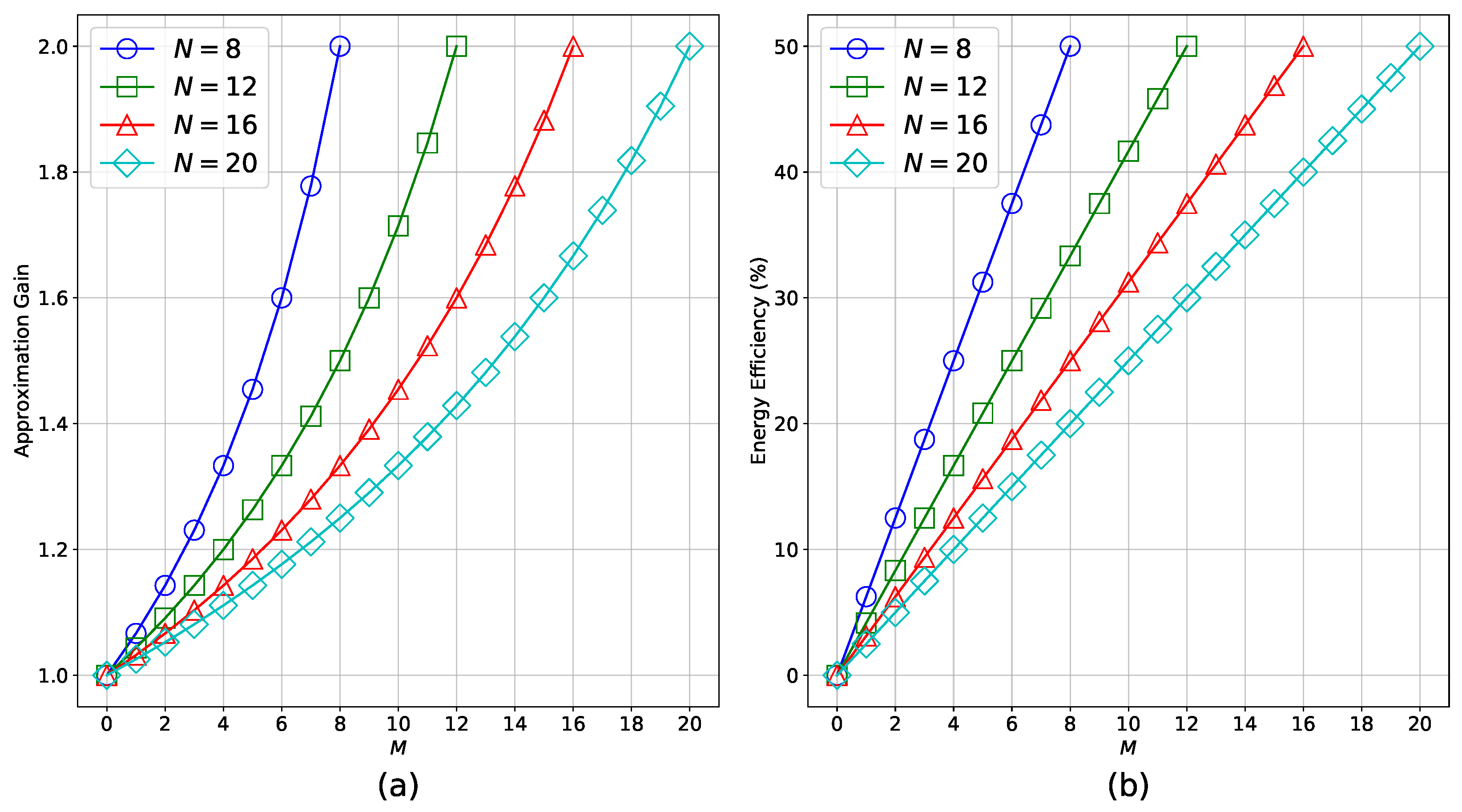
| Approximation | Approximation Gain | ; | As shown in Figure 8a, approximation gain increases with M for all N, while the rate of increase decreases with N. |
| Approximation | Energy Efficiency | ; | As shown in Figure 8b, energy efficiency increases with M for all N, while the rate of increase decreases with N. |
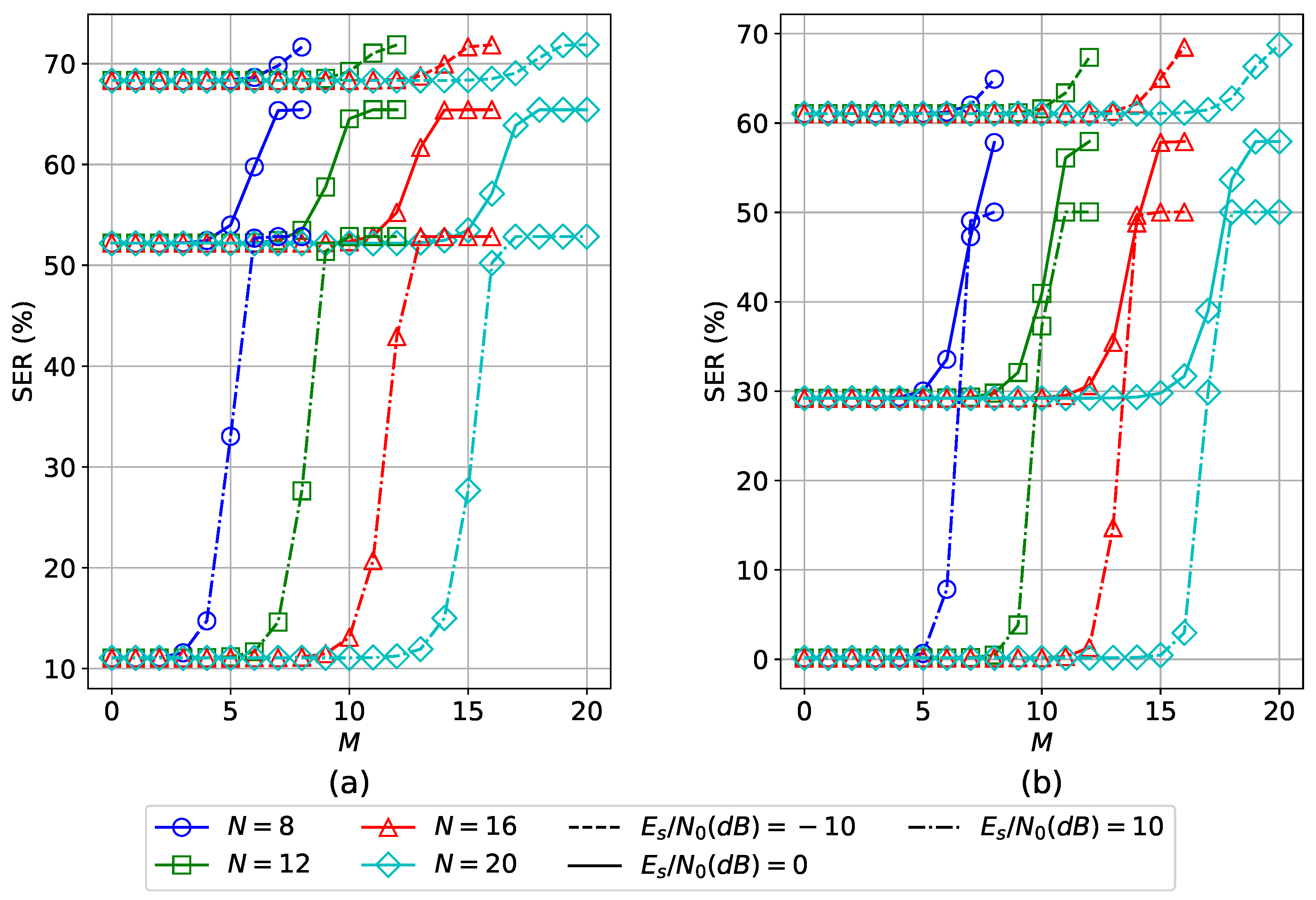
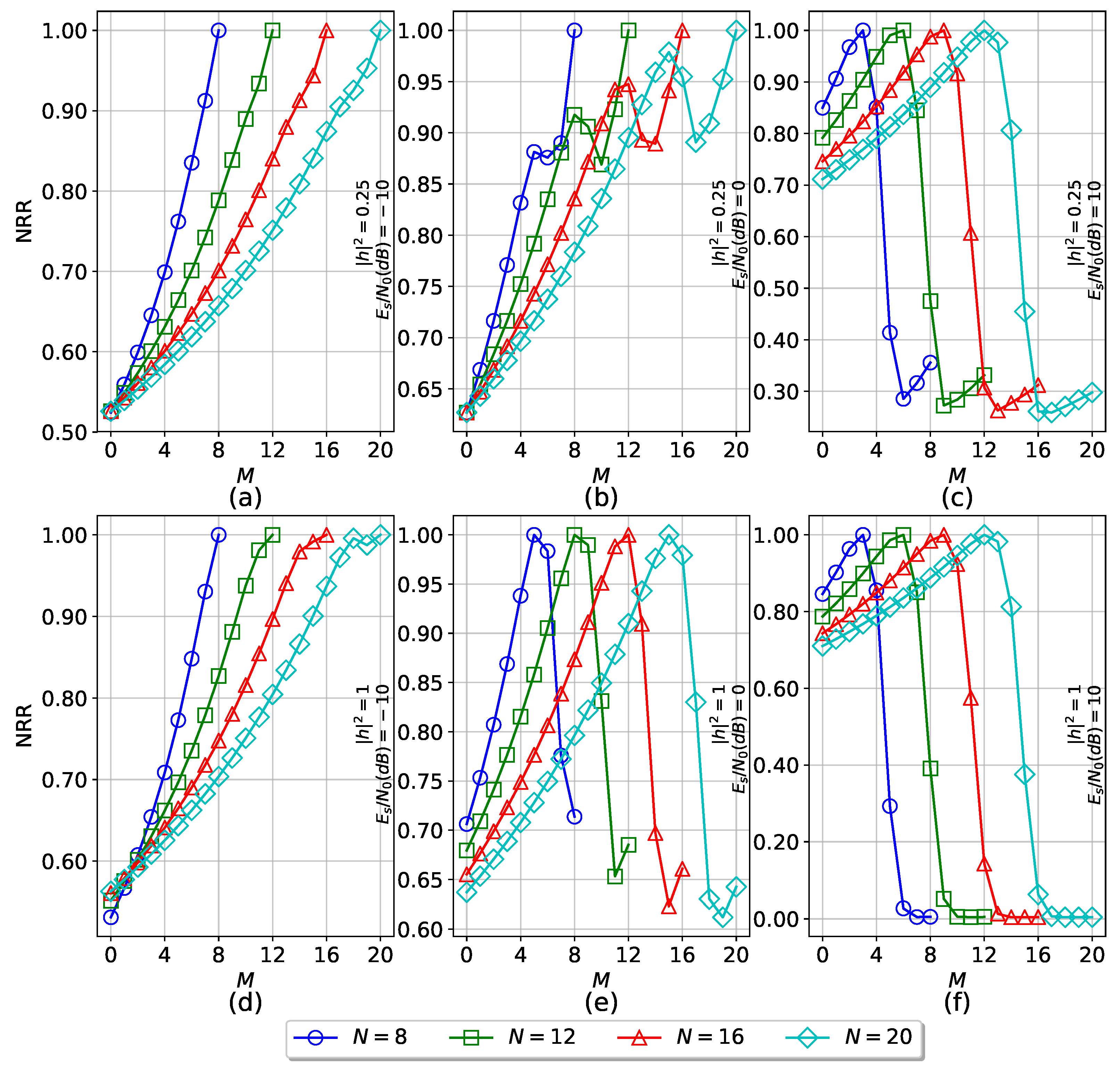
| Resiliency | NRR | ; ; ; | As shown in Figure 9, high NRR is achieved by low M in high SNR regime and high M in low SNR regime. |
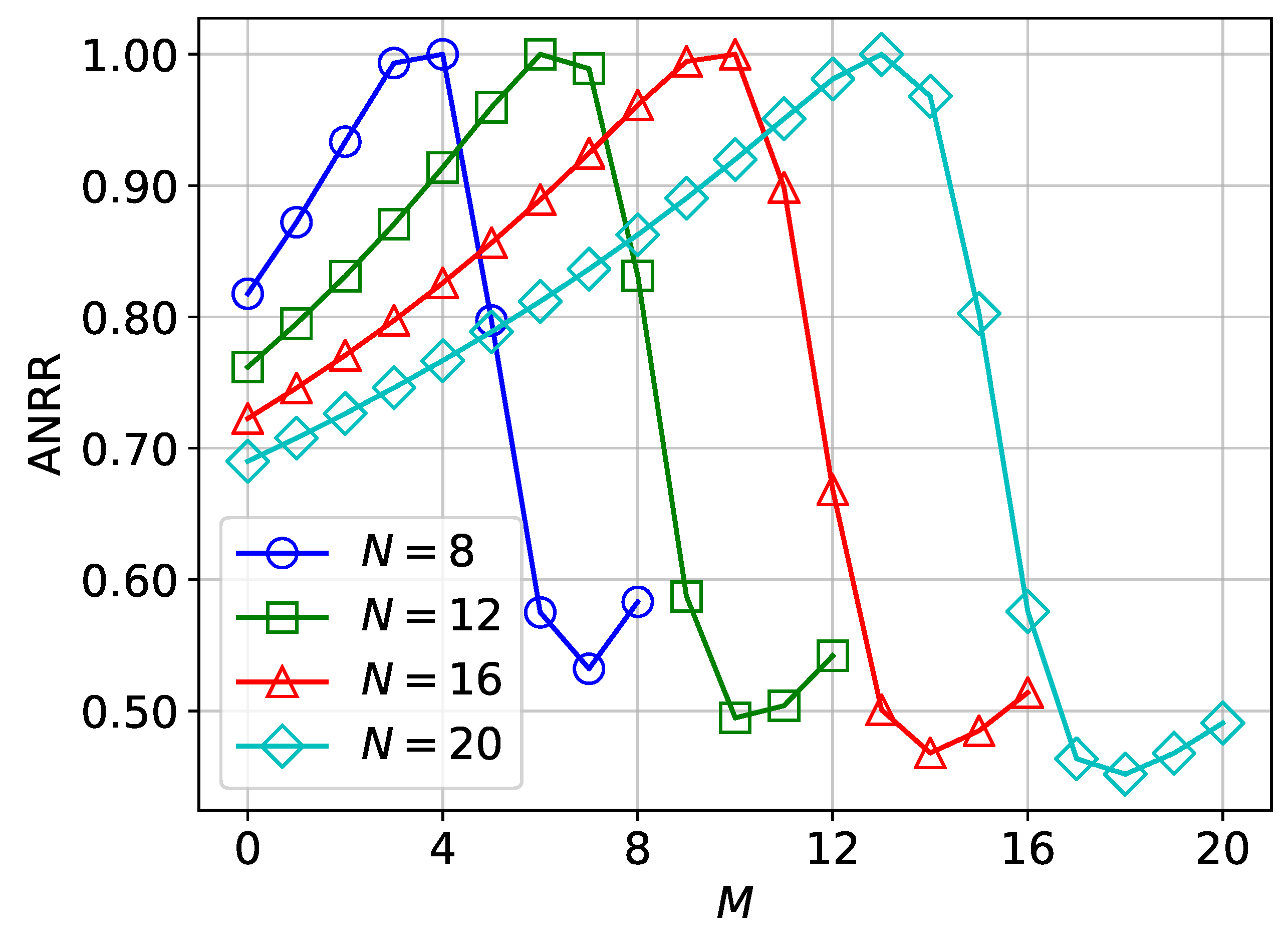
| Resiliency | ANRR | ; ; ; | As shown in Figure 10, rate of increase in ANRR decreases with N and resiliency dips increase with N. |
Disclaimer/Publisher’s Note: The statements, opinions and data contained in all publications are solely those of the individual author(s) and contributor(s) and not of MDPI and/or the editor(s). MDPI and/or the editor(s) disclaim responsibility for any injury to people or property resulting from any ideas, methods, instructions or products referred to in the content. |
© 2024 by the authors. Licensee MDPI, Basel, Switzerland. This article is an open access article distributed under the terms and conditions of the Creative Commons Attribution (CC BY) license (https://creativecommons.org/licenses/by/4.0/).
Share and Cite
Kulkarni, A.; Ouameur, M.A.; Massicotte, D. Energy Efficient Wireless Signal Detection: A Revisit through the Lens of Approximate Computing. Electronics 2024, 13, 1274. https://doi.org/10.3390/electronics13071274
Kulkarni A, Ouameur MA, Massicotte D. Energy Efficient Wireless Signal Detection: A Revisit through the Lens of Approximate Computing. Electronics. 2024; 13(7):1274. https://doi.org/10.3390/electronics13071274
Chicago/Turabian StyleKulkarni, Abhinav, Messaoud Ahmed Ouameur, and Daniel Massicotte. 2024. "Energy Efficient Wireless Signal Detection: A Revisit through the Lens of Approximate Computing" Electronics 13, no. 7: 1274. https://doi.org/10.3390/electronics13071274