Study on Landslide Displacement Prediction Considering Inducement under Composite Model Optimization

Abstract

The precise extraction of displacement time series for complex landslides poses significant challenges, and conventional landslide prediction models often overlook the deformation impacts of displacement triggers. To address this, we introduce a novel composite model tailored for predicting landslide displacement. This model employs Variational Mode Decomposition (VMD) to isolate each displacement component, with optimization achieved through the groupwise coupling algorithm. Subsequently, Grey correlation analysis (GRA) is applied to quantitatively assess the dynamic correlations between various triggering factors and landslide displacement. This analysis informs the construction of a feature set predicated on these correlation factors. Integrating the time-series VMD module into the standard Transformer architecture facilitates the prediction of landslide displacement. This integration allows for the extraction of critical time-evolution features associated with the displacement components. Ultimately, the predicted displacements are aggregated and reconstructed. We validate our model using the Bazimen landslide case study, analyzing displacement monitoring data from 1 January 2007, to 31 December 2012. The values of the root mean square error and the mean absolute percentage error were 1.86 and 4.85, respectively. This model offers a more nuanced understanding of the multifaceted causes and evolutionary dynamics underpinning landslide displacement and deformation, thereby markedly enhancing prediction accuracy.

1. Introduction

Being one of the primary geological disasters in China, landslides present a substantial scale and potential harm. A landslide refers to a geological disaster where soil, rock, or a mixture of soil and rock on the ground or slope is displaced due to factors such as the force of gravity and internal earth forces, moving downwards or laterally along a certain sliding surface or zone. The disasters caused by landslides are extremely severe, and once they occur, they can result in mass casualties, property damage, ecological environmental destruction, and other dire consequences. Accurate prediction of landslides has become crucial for timely response to dynamic situations and ensuring the safety of people’s lives and property. Accurate displacement prediction can issue early warnings hours or even days in advance, providing valuable time for evacuation and thus reducing casualties. For critical infrastructure such as dams, bridges, nuclear power plants, etc., precise displacement prediction can guide necessary reinforcement and maintenance to ensure their stability during disasters, avoiding catastrophic outcomes. Accurate prediction results can also provide a scientific basis for emergency management departments, optimizing resource allocation and rescue plans, and improving the efficiency and success rate of rescue operations. Information about displacement gathered during the evolutionary process of a landslide provides direct insights into the mechanisms and dynamic laws that govern such phenomena. As a result, the prediction of landslide displacement has become a pivotal research focus within the field of disaster prevention and reduction. Accurate displacement prediction can significantly enhance our ability to anticipate and mitigate the risks associated with landslides, thereby saving lives and reducing economic losses in susceptible areas [1,2,3,4,5].

Models for predicting landslide displacement are typically categorized into two main groups: physical models and data-driven models. Physical models incorporate physical mechanisms to predict landslide occurrences through a comprehensive analysis of the physical attributes of the landslide body. However, the generalization ability of physical models is limited, and their effectiveness in long time series predictions does not match that of data-driven models. In recent years, there has been a surge of interest in hybrid prediction models that integrate time series analysis and deep learning techniques. These models have attracted significant attention due to their improved prediction accuracy and generalization capabilities in landslide displacement prediction, surpassing the performance of traditional models. Many intelligent, data-driven, nonlinear models have been utilized in predicting landslide displacement [6,7]. Concurrently, researchers have demonstrated the superiority of the “decomposition–reconstruction–prediction” model approach compared to single prediction models in examining landslide displacement prediction [8]. For instance, Yang. (2022), Guo et al. (2020), and Y. Xing et al. (2019) [9,10,11] utilized a time series analysis method and a variational mode decomposition algorithm (VMD) to decompose cumulative landslide displacement, thereby addressing the issues of incomplete or excessive decomposition when deciphering landslide displacement data. Finally, all projected values are combined to form the predicted cumulative displacement based on the time series model.

Although the composite model above has achieved notable results, there is still room for improvement and some limitations. Considering displacement sequence decomposition, it is worth noting that while the VMD method can perform adaptive decomposition based on data scale and yield highly reliable decomposed slope deformation data, the quality and effectiveness of decomposed data depend on parameter selection [12]. To optimize the precision, robustness, and physical meaning of VMD [13], the VMD method adapts its decomposition approach based on data scale. S. Guan et al. 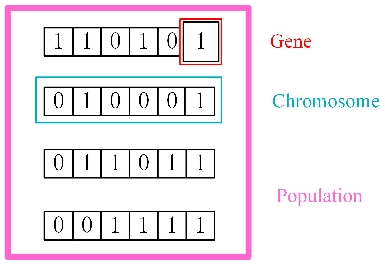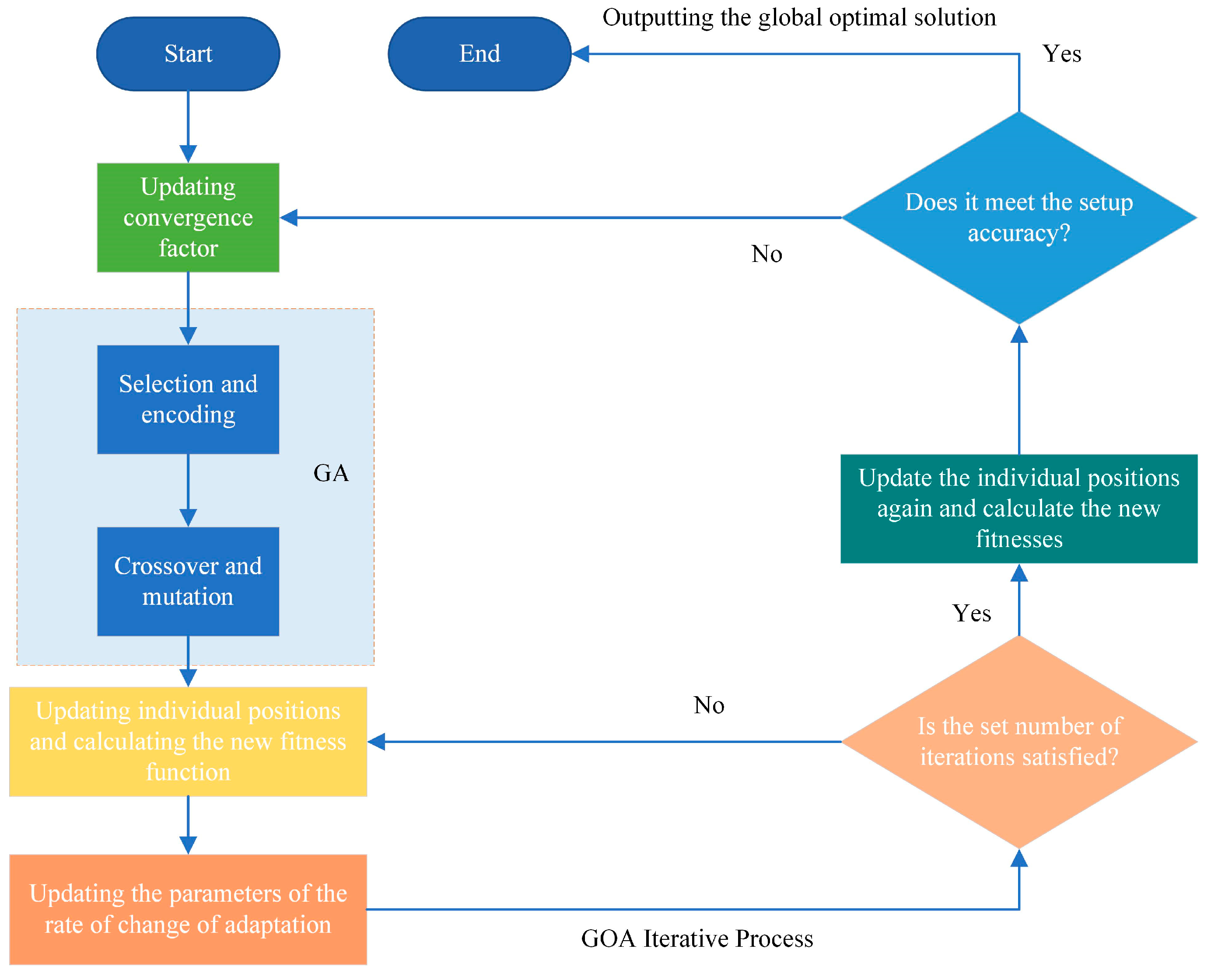have demonstrated that the EMD-PSO-ELM model can effectively measure landslide displacement [14]. In this study, both the genetic algorithm (GA) [15] and the locust optimization algorithm (GOA) [16] are utilized to automatically optimize VMD hyper-parameters. This serves to eliminate the influence of human factors and improve the efficiency of decomposition.

The development of a prediction model is a significant factor influencing the efficacy of landslide displacement prediction [17,18,19]. Time series analysis can be applied to landslide displacement data due to the substantial correlation between past and future data [20,21]. Therefore, incorporating a time series research technique based on deep learning into the prediction of landslide displacement can utilize the temporal correlation between data at different time points, comprehensively understand the evolution mechanism of deformation in landslides, and enhance the accuracy and dependability of forecasts.

Liu et al. (2023) [22] proposed a reliable prediction of reservoir landslides based on an SVR model that responds to triggering factors. Li et al. (2021) [23] proposed a landslide displacement dynamic prediction model based on singular Spectrum Analysis (SSA) and a stacked Long Short Term memory (SLSTM) network. It makes up for the dynamic characteristics of landslide evolution and the shortcomings of traditional static prediction models, and the prediction accuracy is improved. Meng et al. (2023) [24] used a dynamic hybrid model of gated recurrent unit (GRU) and error correction for landslide displacement prediction. It can not only better capture the local change of the accelerated deformation state, but also effectively reduce the extended error in the displacement prediction of long time series.

The aforementioned deep learning network notably improved the accuracy of prediction, but practical application and promotion have limitations. These methods primarily concentrate on “deformation information + an inducing factor” [25] and exclude the appraisal of the physical connotation of each displacement component, the feature data of the triggering factor subsequence, and the interdependence between displacement components and the influencing factor. To address this issue and enhance the comprehensibility of the nonlinear model [26], the proposed solution in this study is to link the major scientific challenge of landslide prediction with a time series network. This involves examining the multivariate time series data to analyze the values of several variables at a given time step and the values of a single variable over multiple time steps. By doing so, the physical interpretability of the model can be improved. Thus, the correlation between factors and the correlation across time intervals can be extracted. The intricate dependence relationship between the landslide displacement input prediction model and the group of feature vectors composed of influencing factors can be analyzed, subsequently improving prediction accuracy.

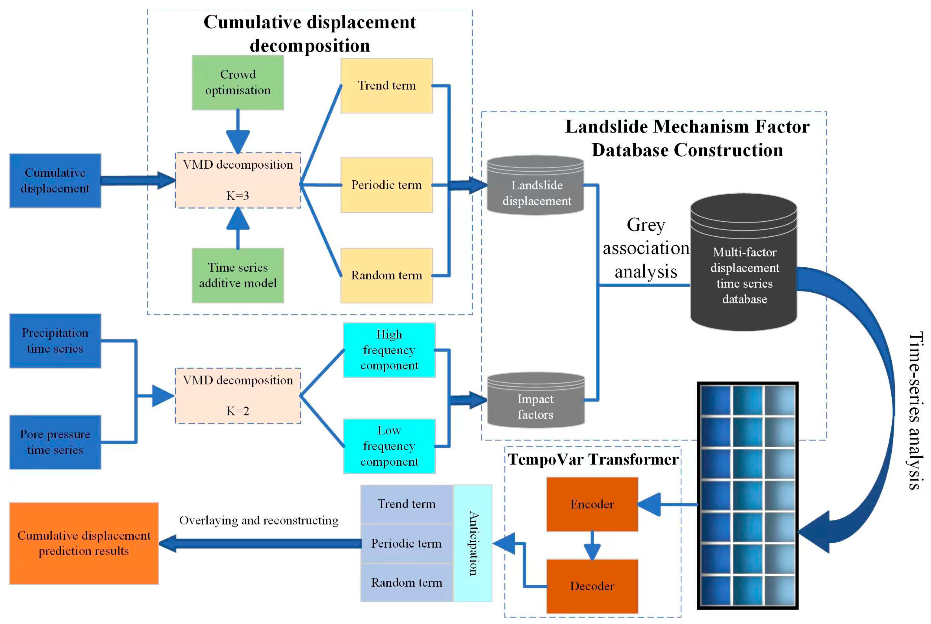
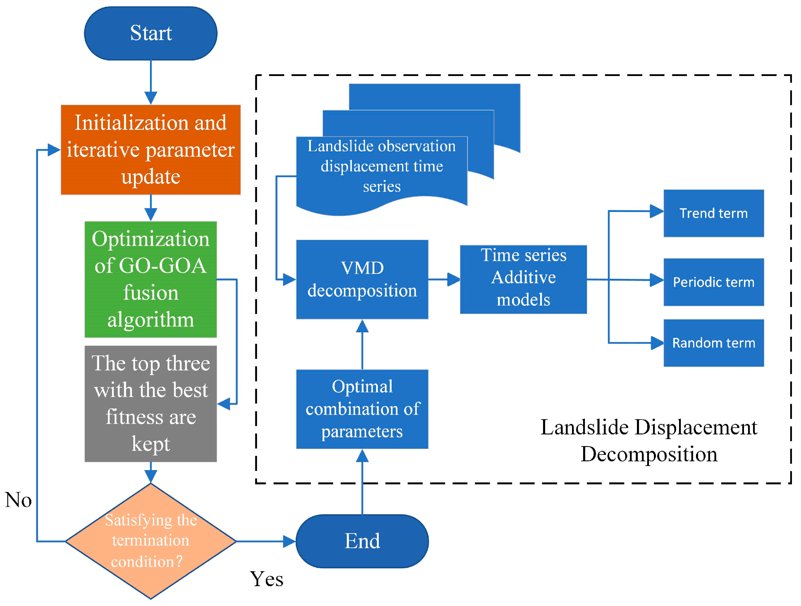
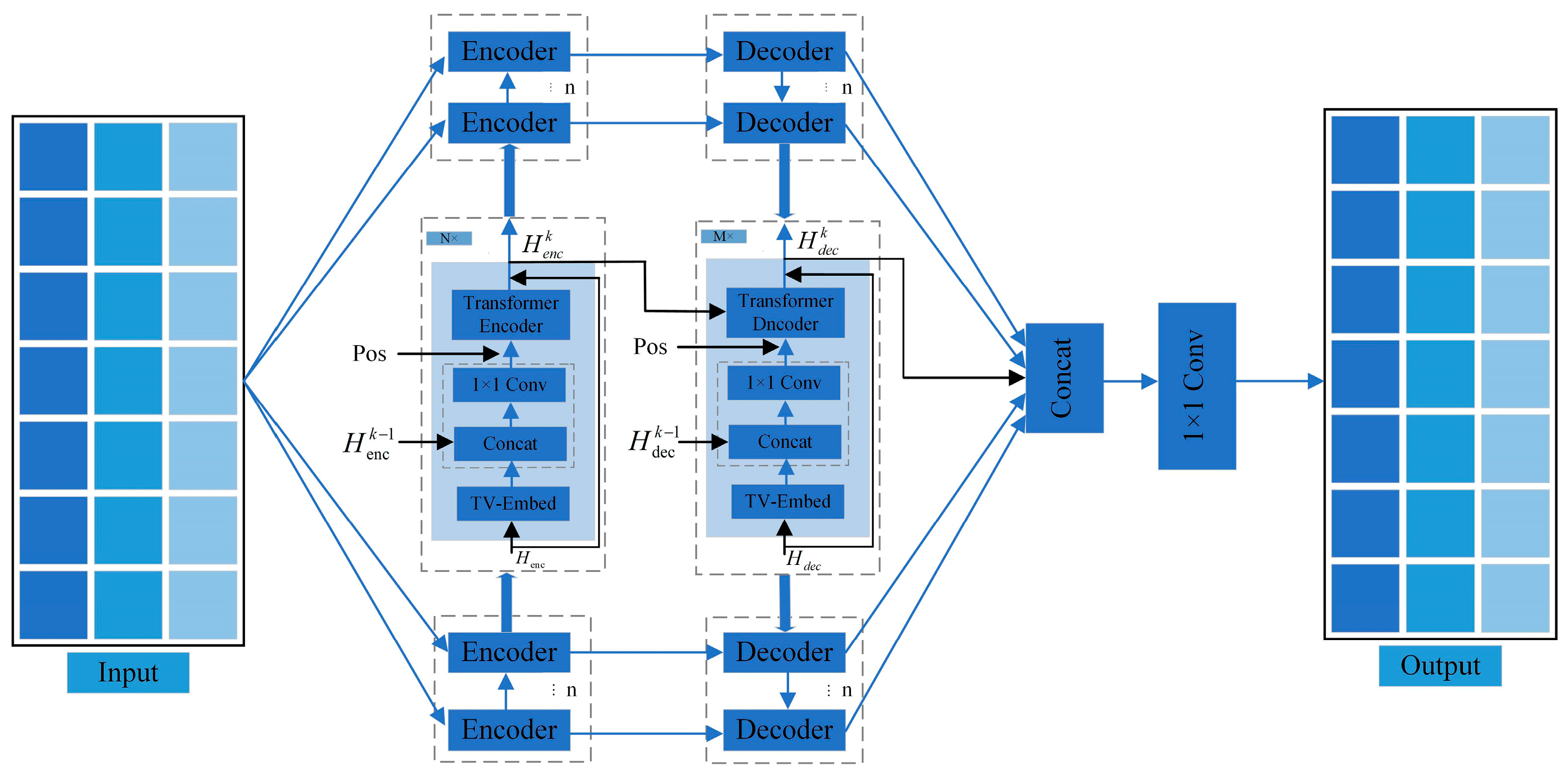
Utilizing the Bazimen landslide dataset from Yichang, Hubei Province, as a case study, this research introduces a composite forecasting framework for analyzing time series data of landslide displacement. The framework begins by decomposing the landslide displacement time series into components with distinct physical meanings and scale characteristics. This decomposition is achieved through the application of time series analysis methods and Variational Mode Decomposition (VMD), which is fine-tuned using a swarm intelligence coupling algorithm. Following the decomposition, a response analysis is conducted to identify the most relevant factors influencing each displacement component. Feature vector groups of various scales are then constructed, reflecting the relationships between the displacement components and their corresponding inducing factors. These groups serve as inputs for the subsequent prediction model. The study proposes a Transformer-based prediction model, enhanced with a time series variability analysis module (TempoVar-Transformer), designed to extract multi-scale information from landslide sequences and integrate it to predict the displacement components with accuracy. The model reconstructs the cumulative displacements of trend, periodic, and random components, and the prediction results are thoroughly evaluated and analyzed to validate the framework’s efficacy.

2. Algorithm in This Paper

The composite model in this paper consists of three modules: the variational mode decomposition module, optimized by the crowd intelligence coupling algorithm; the mechanism factor database construction module; and the TempoVar-Transformer landslide displacement prediction module. Please refer to Figure 1 for a detailed visual representation of the process.

3. Variational Mode Decomposition Optimized by the Coupled Crowd Intelligence Algorithm

3.1. Time Series Additive Model

The evolution of landslide surface displacement deformation over time is a complex outcome influenced by multiple internal and external factors, superimposed on each other [27]. Exploring the dynamic relationships among various influencing factors and landslide deformation in intricate displacement sequence data is a challenging task [28]. Because landslide displacement is influenced by various triggering factors, resulting in a step-type data distribution with nonlinear and non-smooth characteristics, this irregularly varying displacement sequence complicates the fitting of prediction models. To introduce regularity to the input data and enhance the description of the physical significance of landslides, this study preprocesses the time series of landslide displacement. The data are decomposed into trend term displacement affected by internal factors, periodic displacement influenced by external fixed factors, and stochastic displacement impacted by sudden external changes. The displacement time series data are decomposed as follows:

$$X\left(t\right)=A\left(t\right)+B\left(t\right)+C\left(t\right)$$

(1)

where: $X\left(t\right)$ is the observed value of landslide displacement at time $t$; $A\left(t\right)$ is the trend displacement of landslide under the influence of internal factors (material composition, geological structure, topography, etc.) of landslide at time $t$; $B\left(t\right)$ is the cyclic displacement of landslide caused by external influences (seasonal rainfall, change of reservoir level, etc.) of landslide at time $t$; and $C\left(t\right)$ is the stochastic displacement of landslide at time $t$ due to the environmental mutation and error.

3.2. Principle of Variational Mode Decomposition Algorithm

Variational Mode decomposition (VMD) [29] is a new fully adaptive signal decomposition algorithm, which can efficiently decompose nonlinear and non-stationary signals like landslide displacement curve [30]. With a preset number of modes, the input dislocation time series is decomposed into several meaningful components (IMF). The key idea is to create and solve a variational constraint model.

Creating a variational constraint model: The optimization objective is to minimize the sum of the estimated bandwidths of the components. The corresponding constrained variational expression is as follows:

$$\left.\left\{\begin{array}{c}\underset{\left\{u_k\right\},\left\{{\omega }_k\right\}}{min}\hspace{0.17em}\left\{{\displaystyle \sum _{k=1}^K}\hspace{0.17em}{∥{\delta }_t\left[\left(\sigma (t)+\frac{j}{\pi t}\right)u_k(t)\right]e^{-j{\omega }_{t}t}∥}_2^2\right\}\\ s.t.{\displaystyle \sum _{k=1}^K}\hspace{0.17em}{u}_k=f(t)\end{array}\right.\right\}$$

(2)

where, {$u_k\}=\{u_1,\dots ,u_k$} is all modal components obtained after decomposition; {${\omega }_k\}=\{{\omega }_1,\dots ,{\omega }_k$} is the set of its corresponding center frequencies; ${\delta }_t$ is Dirac delta function; * is the convolution operation.

Solving the variational constraint model: Equation (2) is transformed into an unconstrained expression to enhance the saddle point of the Lagrangian function as follows:

$$\begin{array}{c}L\left(\right\{u_k\},\{{\omega }_k\},\lambda )=\\ \alpha \Sigma \parallel {\partial }_t\left[\left(\sigma (t)+\frac{j}{\pi t}\right)u_k(t)\right]e^{-j{\omega }_{k}t}{\parallel }_2^2+\\ \parallel f(t)-{\displaystyle \sum _k}\hspace{0.17em}{u}_k\left(t\right){\parallel }_2^2+\left|\lambda (t),\hspace{0.17em}f(t)-{\displaystyle \sum _k}\hspace{0.17em}{u}_k\left(t\right)\right|\end{array}$$

(3)

where, λ represents the Lagrange multiplier and α represents the penalty parameter.

Finally, the input sequence is decomposed into K components by iteratively updating each modal component {$u_k$} and the corresponding center frequency {${\omega }_k$} using the alternating direction method of multipliers until the iteration condition is satisfied.

3.3. GOA-GA-VMD Fusion Optimization Algorithm

Following the VMD principle, physically significant time series components can be acquired by breaking down the processed landslide displacement data using the VMD algorithm. To ensure interpretability and enforceability, K = 3 is manually specified, which preserves the three modes of trend, periodic, and random items without significant loss of information. The α over-parameter penalty factor and the ascending step size τ in the VMD algorithm strongly influence the quality and effect of the decomposed data. However, the method of artificial determination remains uncertain. Thus, the efficient and accurate selection of parameter combinations is crucial for effectively decomposing landslide displacement sequences using the VMD algorithm. Therefore, this paper proposes to use a swarm intelligence algorithm to effectively solve complex optimization problems and optimize to determine the best parameter combination [α, τ].

The grasshopper optimization algorithm (GOA) simulates the predatory behavior of grasshoppers in nature. Locusts’ biological characteristics include the ability to search for food throughout their life cycle. Local search and global search were carried out simultaneously by taking advantage of the slow movement of larvae and rapid movement of adults [31]. Combining this feature, the location update model of locusts is defined as follows.

$$X_d^i=c_2\left[\sum _{j=1}^N\hspace{0.17em}{c}_1\frac{u{b}_d-l{b}_d}{2}s\left(\left|x_j^d-x_i^d\right|\frac{x_j-x_i}{d_{ij}}\right)\right]+{\widehat{T}}_d$$

(4)

where, $X_d^i$ represents the location information of individual $i$ on dimension $d$, $\left[b_d,l{b}_d\right]$ represents the upper and lower bounds of the search within the individual dimension $d$,|$X_j^d-X_i^d$| represents the relative distance of individual $i$, $j$ in dimension $d$, ${(X}_j-X_j$)/$X_{ij}$ represents the unit vector of individual $i$, $j$, ${\hat{T}}_d$ represents the optimal solution found by the current population, $C_2$ reduces the search trend at the optimal position, $C_1$ to reduce the repulsive force and attraction between locusts, and $s$ is the population interaction force strength function $S\left(r\right)$, which is defined as follows:

$$S\left(r\right)=f{e}^{\frac{-r}{l}}-e^{-r}$$

(5)

where, f is the attraction strength, l is the attractive step size.

The genetic algorithm (GA) is a multi-point search global optimization algorithm based on the principles of biological evolution. In this algorithm, the problem parameters are encoded as chromosomes. The initialization coding schematic is shown in Figure 2. Subsequently, the selection, crossover, and mutation operations are carried out iteratively to exchange chromosome information in the population. Finally, the chromosomes aligned with the optimization goal are generated [32]. The algorithm consists of four parts: parameter coding, initial population setting, fitness function design, and selection, crossover, and mutation operation. In this paper, the fitness function is defined as the error between the predicted value and the expected value of the VMD hyper-parameter. The algorithm can quickly converge to the globally optimal solution.

GA is commonly employed as a global optimization algorithm, excelling in solving global optimization problems and possessing robust global search capabilities. However, GA is less effective in local search and is prone to converging to local optimal solutions. Additionally, GA lacks memory ability. If the population changes during the iteration process, the previous information will be lost [33]. In contrast, GOA possesses memory ability. At each iteration, the population utilizes the individual extreme value and the group extreme value to update its speed, position, and fitness value, aiding in retaining the optimal solution. However, GOA is susceptible to premature convergence and may lose population diversity. GA can preserve population diversity through crossover and mutation operations [34].

The advantages of the two algorithms complement each other. Firstly, GA has the ability to search globally, and it is utilized to select the optimal chromosome for forming the best population. Subsequently, GOA applies its local search ability to select the optimal individual and, through continuous iterative updates, returns the optimal weight threshold. This approach effectively enhances the search accuracy and convergence speed of the VMD hyper-parameter group. The algorithm coupling process is displayed in Figure 3, while Figure 4 illustrates the GA-GOA-VMD decomposition process.

4. Trigger Database Construction

During the extraction of information on landslides, a significant amount of deformation data and redundant information is often present, which could impede the predictive accuracy of the model. Failure to eliminate these superfluous details diminishes the model’s ability to generalize, resulting in decreased prediction accuracy. To address this issue, the current study utilizes the Grey correlation analysis (GRA) method [35] to extract potential impact factors from both periodic and random displacement components, creating a database of trigger factors. Subsequently, the VMD algorithm is optimized to decompose each factor sequence into high and low frequency components. The correlation coefficients between periodic and random components, as well as the high and low frequency components of the trigger factor, were computed. Ultimately, the most significant trigger factors of periodic and random items were selected to create the time series feature vector group and feed it into the prediction model.

5. Landslide Displacement Prediction

5.1. Time Series Variable Analysis Module

To fully capture the concealed information dependencies within the multivariate Temporal feature vector group, which includes inducing factors and deformation displacements, this paper introduces a temporal variable module as the input operation of the TempoVar-transformer prediction model, as depicted in Figure 5.

The landslide dislocation-time series $X$ is set to have $I$ time points, and each time step has $D$ features. This module uses a one-dimensional Conv neural network with a convolution kernel size of 3 × 1 to process the information of multivariate time series into the feature map, while keeping the spatial and temporal dimensions unchanged, as follows:

$$X_{emb}=Conv\left(X_{input}\right)$$

(6)

where, $X_{input}$ stands for $X_{cycle}$ (periodic term component) or $X_{random}$ (random term component); $X_{emb}$ is the feature vector group composed of inducing factors and displacement vectors.

In order to extract the local information in the sequence, the feature map is divided into small blocks with specific scale by $Patch$ (block) operation. When the length of the feature vector of the displacement time series is not divisible by $P$ of size $Patch$, zero-padding is performed at the end of the time series, known as the $Pad$ operation in the figure. The $Patch$ procedure divides the corrected time series into $N=\raisebox{1ex}{$I$}\!\left/ \!\raisebox{-1ex}{$P$}\right.$ blocks of size $P$ non-overlapping $Patch$. The operations are defined as follows:

$$X_{emb}=Patch\left(X_{emb},X_0,P\right)$$

(7)

where $P$ is the length of each $Patch$, $X_0$ means zero padding.

5.2. TempoVar-Transformer

In this paper, the standard Transformer [36] is improved into the TempoVar-Transformer architecture of Figure 6 with multi-layer embedded temporal variable analysis module, which contains multiple encoder–decoder pairs. The input at each level is the same, and encoders at different levels learn different levels of feature representations.

The time series variable analysis module converts the input data $X_{enc}$ into a blocked feature map representation, denoted as $X_{di}^k$, which is defined as follows:

$$X_{di}^k=TV\left(X_{enc},P_k\right)$$

(8)

where, $P_k$ represents the specific Patch size adopted when processing the input data.

Then, a cross layer connection mechanism is introduced between different levels, and the input $X_{di}^k$ of the first level encoder is cascaded with the output $H_{enc}^{k-1}$ of the lower level to effectively aggregate the landslide feature information of different levels, so as to process the spatio-temporal data of displacement sequence more effectively. The diagram is as follows:

$$X_{emb}^k=\left\{\begin{array}{ccc}{X}_{di}^k& if& k=1\\ Corn\left(Concat\right(X_{di}^k,H_{enc}^{k-1}\left)\right)& if& k\ne 1\end{array}\right.$$

(9)

where, $X_{emb}^k$ is the feature information output by encoders at different levels; $Concat$ represents the concatenation process along the feature map dimensions; $Conv$ means using a 1 × 1 convolution kernel to fuse and reduce the dimension of the connected feature map.

Furthermore, since the Transformer architecture has the natural property of being “order-independent”, this means that it does not explicitly consider the relative position of elements in the input sequence. Therefore, to capture the temporal dependencies inside the input sequence, we propose to add learnable position matrices $W_{pos}^k$ to $X_{emb}^k$, assigning a specific encoding vector to each time step to distinguish the temporal order of the data. The output is the temporal relationship between the captured landslide univariate series data.

$$X_{emb}^k=X_{emb}^k+W_{pos}^k$$

(10)

where, $W_{pos}^k$ represents the encoding matrix at a specific time step.

Transformers are built on self-attention mechanisms, which allow them to inherently extract features and capture long-term dependencies without the need for recurrent networks or convolutional layers. They operate by employing the query-value-key paradigm, where keys are compared to a query to assign attention weights to their corresponding values. In the context of this paper, the initial sections of the model have already selected favorable characteristics from the landslide sequence.

Hence, the paper employs the dot product attention mechanism with conventional encoder scaling and the multi-head attention mechanism to process multivariate time series displacement data with varying time steps. This approach enables the model to concentrate on the information most relevant to the current position in the input sequence, while still maintaining the ability to recognize and integrate diverse sequence characteristics. By doing so, the model can effectively leverage the temporal dependencies and structural features of the data, leading to more precise predictions of landslide displacement.

The input of the Decoder is a time series of the history record $L$ time steps and the future $H$ time steps concatenated, denoted as $X_{dec}^k$. The output of the decoder is denoted as $H_{dec}^k$, and the number of $Patch$ is $N_{dec}^k$ blocks. Since we mainly focus on the prediction task of displacement time series, only feature representations at future time steps are needed, and the number $Patch$ of future time steps is block $N_{pred}^k$, which is defined as follows.

$$N_{dec}^k=\frac{L+H}{P_k}$$

(11)

$$N_{pred}^k=\frac{H}{P_k}$$

(12)

Finally, the latent representations of all levels are concatenated and the prediction $X_{pred}$ is generated using the Conv layer, as shown here:

$$H=Concat\left(H_{dec}^1,\dots ,H_{dec}^k\right)$$

(13)

$$X_{pred}=Conv\left(H\right)$$

(14)

The encoder–decoder structure of the TempoVar Transformer model can pay attention to the relationship between different time steps and features at the same time, which helps the model to gain a better understanding of the internal structure and law of the data, so as to extract useful information and features in the time series relationship, and deal better with the complex and variable landslide displacement prediction problem.

5.3. Model Structure

In the field of machine learning and data science, understanding the key parameters of each algorithm is crucial to optimize the performance of the model, and it is also important to conduct our experiments. Therefore, we comb the input, output, and hierarchical structure of all our algorithms in

Table 1. Hierarchical architecture diagram of all model inputs and outputs.

Model	Input	Output	Hierarchical Structure
VMD	Cumulative displacement time series data	Various displacement time series data	Probability distribution estimation, variational inference
GA	Constrained objective function	The global optimal solution	Population initialization, fitness evaluation, selection, crossover, mutation
GOA	Constrained objective function	Local optimal solution	Population initialization, pheromone update, state transition rule
GRA	Time series for analysis and comparison	Degree of association	Data preprocessing, correlation calculation
TempoVar-Transformer	Displacement and impact factor time series data	Time series data for predicting displacement	Multi-head self-attention mechanism, encoder-decoder structure, positional encoding

.

6. Slippery Slope Analysis and Example Application of the Bazimen Landslide

6.1. Geological Profile of the Bazimen Landslide

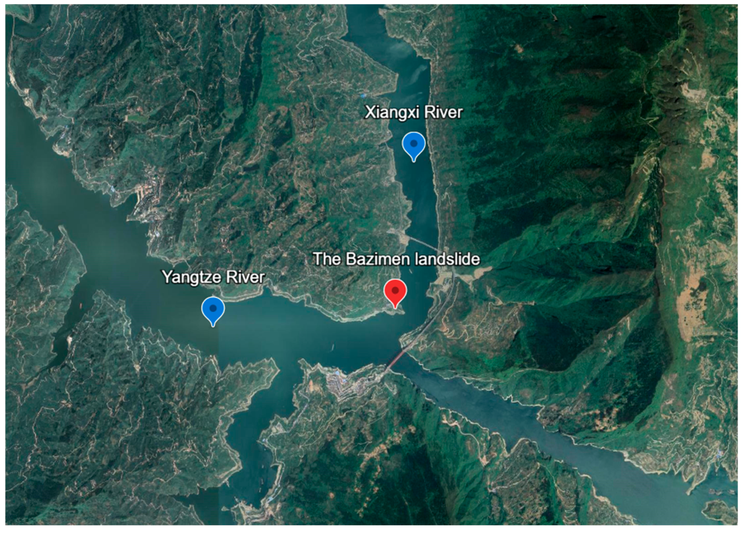
The Bazimen landslide (110°45′ E, 30°58′ N) is located in Xiangxi Village, Guizhou Town, Zigui County, Hubei Province, within the Three Gorges Reservoir area, approximately 38 km from the Three Gorges Dam. Located on the right bank of the Xiangxi River, 0.8 km from its confluence with the Yangtze River, the slope morphology resembles an irregular fan. Homologous alluvial gullies develop on both sides of the boundaries, forming a circular trailing edge and a water facing leading edge. The longitudinal length of the landslide is 550 m, with a narrow top and a wide bottom, covering a total area of 13.5 × 10⁴ m². The average thickness of the landslide body is around 30 m, with a total volume of approximately 400 × 10⁴ m³. The slope ranges from 40° to 60°, and the landslide body mainly consists of a yellowish-brown, purplish-red, and dark grey fragmented stone soil layer, composed of blocks, gravels, and pulverized clay. The structure of the landslide body is loosely accumulated, and unfavorable factors such as rainfall and upper catchment water scouring can impact the stability of the entire landslide area, making it prone to overall instability-induced landslides. The Bazimen landslides are located in a subtropical monsoon climate, experiencing year-round rainy weather, with rainfall being a significant factor influencing landslide displacement. The Bazimen landslide entered its initial resurrection stage during the Gezhouba dam water storage in 1981. Since 2003, with the Three Gorges Dam water storage, Bazimen landslides have exhibited noticeable deformation. During the rainy season from May to July 2004, coupled with a drop in the Three Gorges reservoir level, shear cracks formed in the middle and upper parts of the landslide. The landslides are frequently active during the annual rainy season, primarily located in the middle and at the back edge, significantly affecting the normal life and access of neighboring areas. 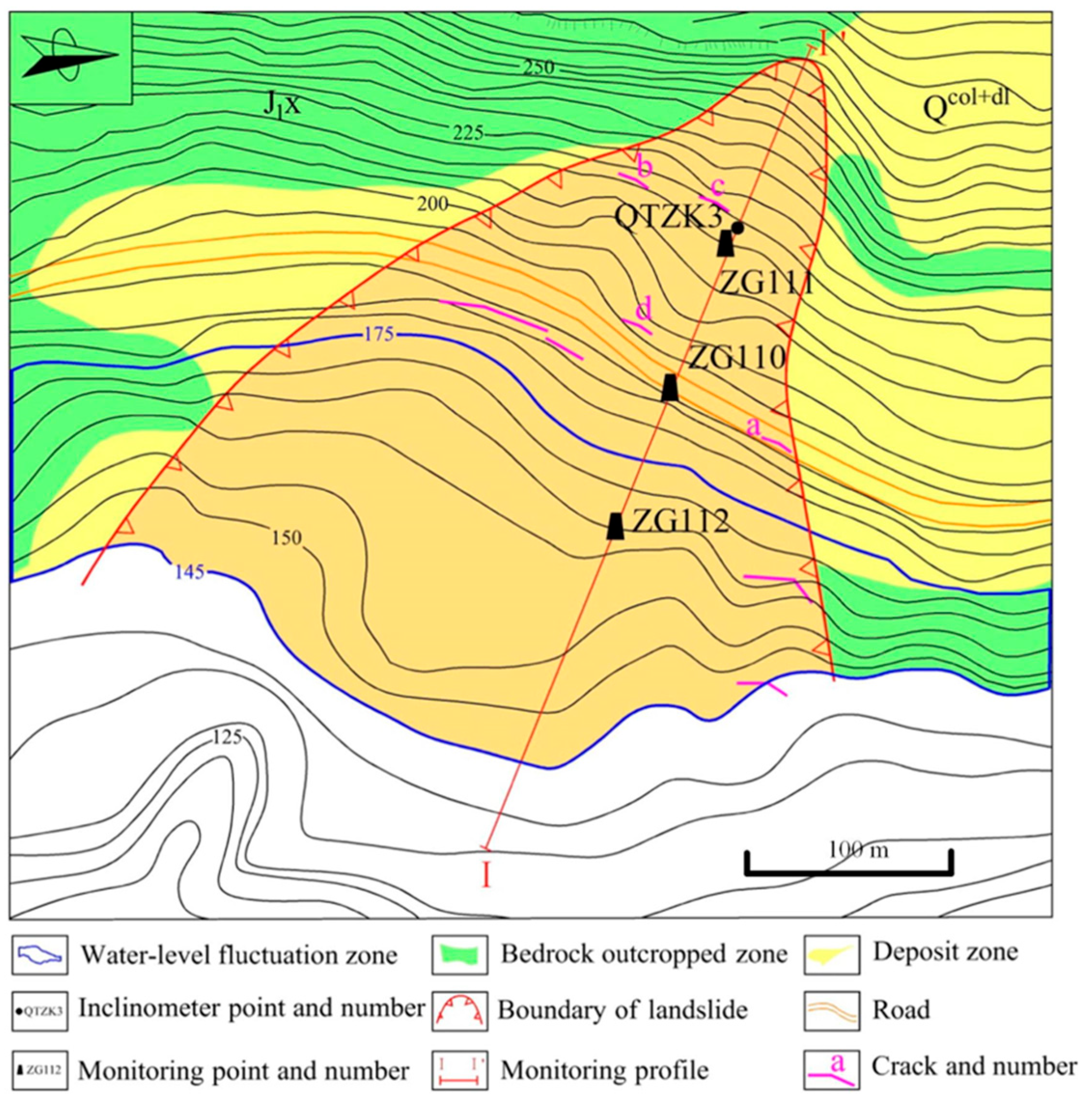The satellite map of the Bazimen landslide is shown in Figure 7, and its planar contour map is shown in Figure 8.

6.2. Characterization of Landslide Deformation Based on Monitoring Data

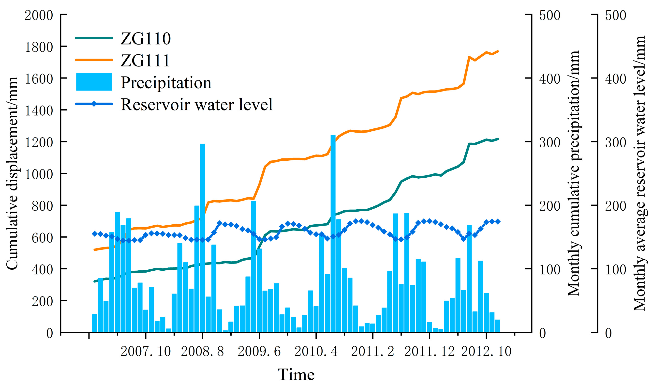
Two GPS deformation monitoring points (ZG111, ZG110) were strategically placed in the landslide area, and data were obtained from the National Field Scientific Observation and Research Station of the Three Gorges Landslide of the Yangtze River in Hubei Province. The dataset initiation coincided with the impoundment of the water level in front of the Three Gorges Dam to 135 m in mid-June 2003. Subsequent monitoring took place monthly. The timeline of the Bazimen Landslide Displacement Monitoring Points is illustrated in Figure 9, depicting the cumulative displacement-reservoir level-rainfall curve at the Bazimen landslide displacement monitoring point. The utilized data cover the period from January 2007 to December 2012. Analysis of the monitoring data reveals that during periods of low rainfall each year (January 2007 to March 2007, October 2007 to March 2008, November 2008 to March 2009, October 2009 to April 2010, November 2010 to April 2011, December 2011 to April 2012, October 2012 to December 2012), the time accumulated displacement-reservoir level-displacement curves at the Bazimen landslide monitoring site are delineated. In contrast, during periods of elevated and concentrated rainfall (April to July 2007, July to August 2008, May to June 2009, May to August 2010, June to August 2011), the cumulative displacement exhibited rapid, step like increments. Notably, the “step period” and concentrated rainfall periods each year did not precisely align. A time lag between the “step period” and concentrated rainfall period is evident, signifying that the landslide displacement “step” occurs subsequent to continuous or heavy rainfall—a pattern observed consistently. During “step” periods, significant changes in the reservoir water level were also noted. For instance, from April 2008 to September 2008, the reservoir water level experienced a decline, followed by an increase from September 2008 to November 2008. In this period, from April 2008 to November 2008, the cumulative displacement of the landslide exhibited a sudden increasing trend. Similar patterns were observed in other time periods. It is evident that the primary factors influencing Bazimen landslide displacement are rainfall and reservoir water level.

6.3. Analysis of Influencing Factors

Choosing appropriate triggering factors for landslides is crucial for the accuracy of predictions, especially for predicting periodic components. Studies have shown that rainfall and reservoir water level are the main triggering factors for landslides in the Three Gorges Reservoir area [37,38], and Bazimen landslide is located in this area. Rainfall increases soil pore water pressure, thereby reducing the effective stress of the soil. When the effective stress of the soil decreases to a certain extent, the shear strength of the soil mass also decreases, making it prone to landslide occurrence. Additionally, rainfall saturates the soil, increasing its weight, which in turn increases the downslope force, further promoting landslide occurrence. Changes in reservoir water level can cause changes in groundwater levels, further affecting soil pore water pressure and effective stress. By comparing the changes in landslide displacement deformation with rainfall and reservoir water level changes, it can be seen that months with concentrated rainfall and stages with significant changes in reservoir water level can lead to larger deformations of landslides.

Landslides are complex natural phenomena that are undoubtedly caused by a combination of multiple factors, such as soil, geological structure, groundwater, and human activities, among others. However, this study did not consider other factors for several reasons. Firstly, the changes in other factors are more random and difficult to capture regular patterns, and their general impact is smaller. Secondly, our composite model, when using rainfall and reservoir water level as the dominant triggering factors, decomposes the displacement into three components: trend term, periodic term, and random term. The periodic term displacement is key and depends on the dominant factor, while the random term displacement includes not only some noise errors but also other small influencing factors from the perspective of landslide mechanisms. Finally, by reconstructing all terms, we obtain the total predicted displacement, which also shows that our model has a high degree of tolerance and robustness, with practical significance.

6.4. Evaluation Index

In order to accurately evaluate the prediction effect of our designed model, the evaluation metrics are Root Mean Square Error ($RMSE$) and Mean Absolute Percentage Error ($MAPE)$,which are defined as follows:

$$RMSE=\sqrt{\frac{1}{N}\sum _{i=1}^N\hspace{0.17em}{\left({\widehat{d}}_t-d_t\right)}^2}$$

(15)

$$MAPE=\frac{100\%}{n}\sum _{i=1}^n\hspace{0.17em}\left|\frac{{\widehat{d}}_t-d_t}{d_t}\right|$$

(16)

where, $N$ is the size of the predicted sample, $d_t$ is the actual value at time $t$, $d_t$ is the predicted value at time $t$, and $\overline{d_t}$ is the arithmetic mean of all the actual values.

The range of $RMSE$ is $\left[0,+\infty \right]$, the smaller the value, the stronger the model fitting ability; The range of $MAPE$ is $\left[0,+\infty \right]$, where an $MAPE$ of 0% indicates a perfect model, and an $MAPE$ greater than 100% suggests a poor-quality model. When both $RMSE$ and $MAPE$ are sufficiently small, it indicates that the predictive model has a good forecasting performance.

6.5. Assumptions and Limitations

This section discusses the assumptions and limitations of the research presented in this paper. We aim to provide readers with a transparent and comprehensive understanding of our research methodology, and to assist them in evaluating the applicability and credibility of our research results in real-world applications.

6.5.1. Assumptions

We assume that the displacement of landslides is primarily influenced by the selected input variables (rainfall, reservoir water level, past displacement). Although these variables have been widely recognized as key factors affecting landslide displacement, other relevant factors may not be included in the model.

Our model assumes that the quality and integrity of the data are sufficiently high to enable effective training and prediction. However, in reality, the data may contain noise, outliers, or missing values, which could potentially affect the model’s performance.

We assume that the physical processes of landslides remain consistent throughout the study period. This means that we have not considered possible geological changes or long-term impacts of external factors on slope stability.

6.5.2. Limitations

Deep learning models typically require a large amount of data for training, but high-quality long-term time series data may be difficult to obtain in the field of landslide prediction. Consequently, our model may not fully utilize all the information in the data.

Our model does not account for the spatial and temporal variability of landslide displacement. Landslide events may exhibit different characteristics in different regions, which could limit the generalizability of the model.

6.6. Experimental Analysis and Model Comparison

6.6.1. Data Selection

In order to enhance the training of the prediction model in this paper, the selected monitoring point is ZG111, situated in the middle and rear part of the landslide body. This location provides ample data on displacement and deformation, precipitation, reservoir level, and frequent deformation. The research and analysis focus on the data collected during the monitoring period from January 2007 to December 2012. The experimental data are measured in monthly units, with a total of 70 months considered. The first 50 months’ data are designated as the training set for model training and parameter adjustment, while the remaining 20 months’ data serve as the test set for assessing the model’s accuracy. Due to the scarcity of data, we employed a cross-validation approach to evaluate the model’s generalization capability and to avoid overfitting. This method allows us to make the most of the limited data available and provides a more robust assessment of the model’s performance without the need for a separate validation set.

6.6.2. Parameter Optimization

Before performing the optimization, the optimization range of the penalty factor for the hyper-parameter combination of VMD decomposition is set to $\left[1000,\hspace{0.17em}3000\right]$; the optimization range of the rise time step is set to $\left[0,\hspace{0.17em}1\right]$; the population size in the GOA algorithm is set to 100; and the maximum number of iterations is set to 100. The hyper-parameter combination obtained from the final optimization is shown in

Table 2. Optimization results of the Smart Group algorithm for VMD parameters.

Modal Preset	Optimal Parameter Combination
Number of modes	Penalty factor α	Rise time step λ	Fitness value
3	1858	0.365	0.2785

:

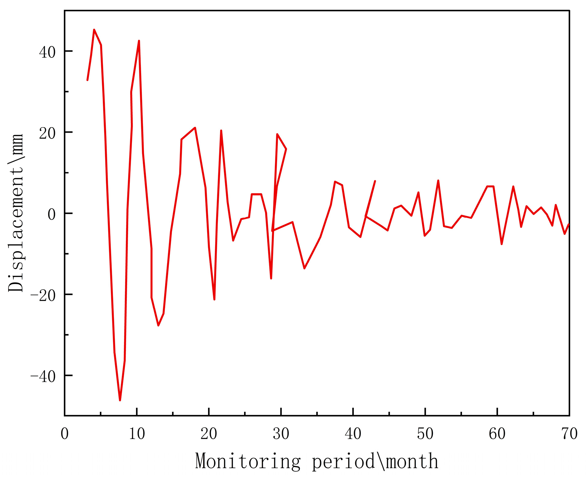
6.6.3. Results of Displacement Sequence Decomposition

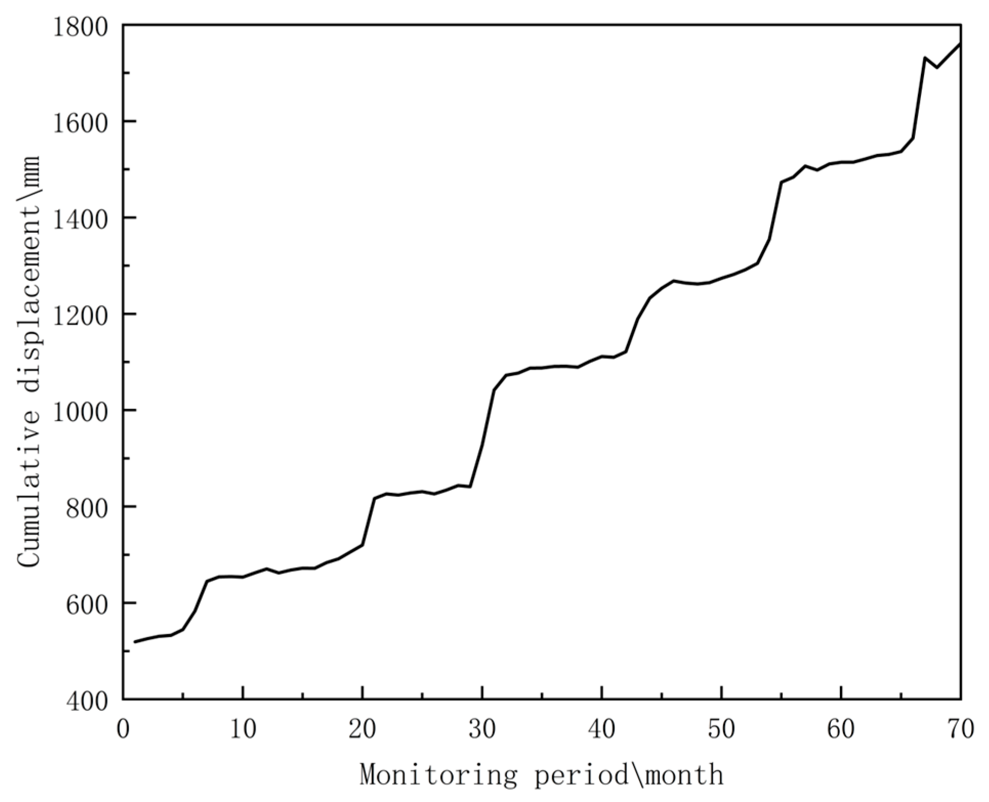
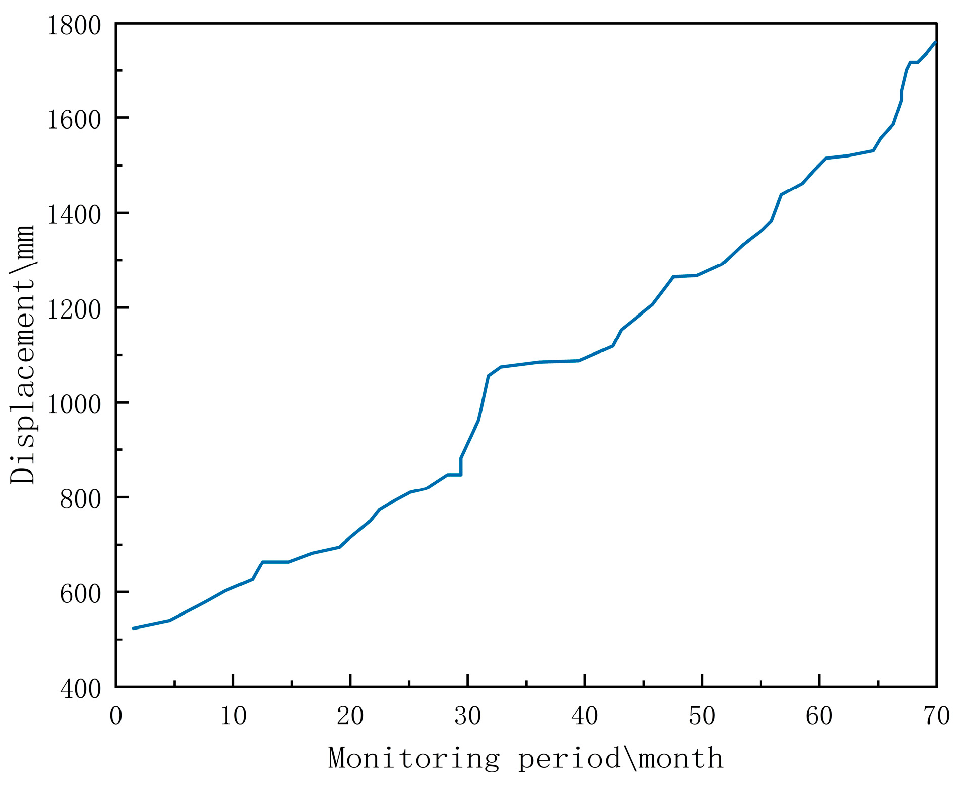
The VMD algorithm, with hyper-parameters obtained through the crowd-wise coupled optimization algorithm in the preceding subsection, is utilized to successively decompose the original cumulative displacement into trend, periodic, and random terms. The total observed displacement is depicted in Figure 10, and the decomposition results are illustrated in Figure 11, Figure 12 and Figure 13, respectively.

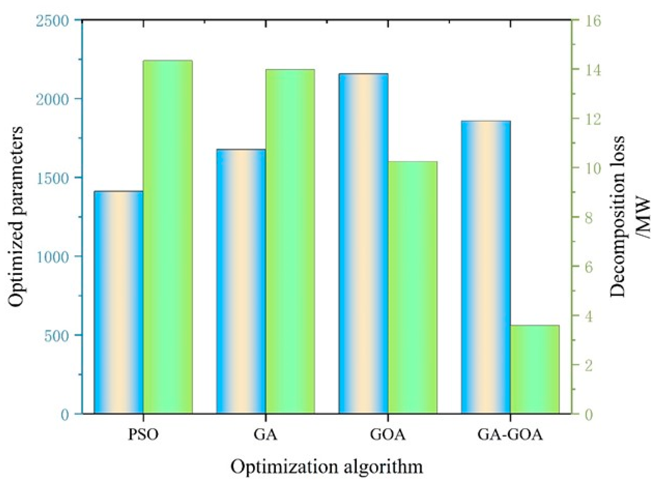
6.6.4. Comparative Experimental Analysis of Coupled Optimal Decomposition Algorithms

To verify that the coupled optimization algorithm proposed in this paper produces better decomposition effect and fidelity for VMD decomposition than traditional optimization algorithms, the following particle swarm optimization algorithm (PSO), genetic algorithm (GA), and locust optimization algorithm (GOA) are selected for comparison with the method of this paper, as shown in

Table 3. Comparison of the effect of VMD combined with other optimization algorithms.

Decomposition Model	Number of Decomposed Modes	α	Decomposition Loss\MW
Original VMD	3	1000	21.85
PSO-VMD	3	1412	14.34
GA-VMD	3	1678	13.98
GOA-VMD	3	2157	10.25
GA-GOA-VMD	3	1858	3.59

and Figure 14:

The comparative results indicate that the combined GOA-GA optimization algorithm minimizes the VMD decomposition loss, ensuring both effective decomposition and fidelity. It can be inferred that the decomposition achieved using either the GOA or GA algorithm alone is less effective than the fusion optimization of the two. This supports the effectiveness of the combined optimization algorithms presented in this paper.

Table 4. Sensitivity analysis of α optimized by the optimization algorithm.

Optimization Algorithm	Reference Value	Range of Variation	Minimum Value	Maximum Value	Sensitivity Ranking
PSO	2000	−39.6%~+6.4%	1209	1872	4
GA	2000	−22.5%~+5.9%	1550	2117	2
GOA	2000	−15.6%~+30.9%	1689	2619	3
GA-GOA	2000	−11.7%~+4%	1766	2080	1

shows the results of the sensitivity analysis performed on each optimization algorithm.

Through sensitivity analysis of the hyperparameters optimized by various optimization algorithms for VMD, it can be observed that the hyperparameters optimized by GOA and PSO have a wide range of variations, which makes VMD prone to mode aliasing and feature loss. This also indicates the superiority of the GA-GOA joint optimization algorithm.

6.6.5. Quantitative Analysis of the Association Degree between Landslide Displacements and Influencing Factors

Utilizing the rainfall and reservoir level data recorded during the same period, the influencing factors underwent Grey correlation analysis with the displacement data. The results are depicted in Figure 15.

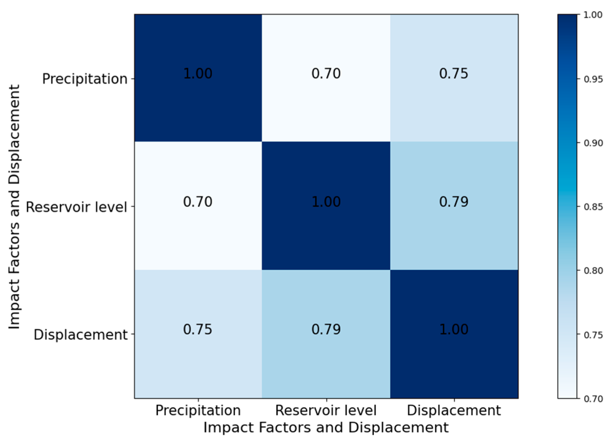
From the confusion matrix in Figure 16, it is evident that the correlation between displacement and rainfall, as well as the reservoir level at monitoring point ZG111 of the Bazimen landslide, are 0.75 and 0.79, respectively. The correlation values exceed 0.7, indicating a strong correlation between landslide changes and rainfall as well as the reservoir level. Consequently, to achieve accurate displacement prediction, these impactful factors cannot be disregarded. Additionally, a correlation of 0.7 is observed between rainfall and reservoir water level, suggesting a relationship between the two. Upon analyzing the evolution process of the landslide, it is evident that rainfall generates surface runoff on the landslide body’s surface. Through infiltration, it elevates the groundwater level, resulting in increased pressure between rock layers. Simultaneously, the rise in reservoir water level amplifies buoyancy forces in the base–cover interface, inducing significant landslide deformation and decreasing stability. As the reservoir water level decreases, the landslide loses the groundwater buoyancy effect, and deformation automatically halts to some extent, leading to increased stability. After substantial rainfall, landslide displacement continues to rise because the groundwater is not entirely evaporated, and the landslide remains in an unbalanced environmental state, as depicted in Figure 9. When the reservoir water level drops to its lowest point, the rate of landslide displacement rise increases. These observations reveal a certain lag in the impact of rainfall and reservoir water level on landslides. Rainfall increases both surface and underground runoff, contributing to reservoir area infiltration, leading to a subsequent rise in reservoir water, exhibiting a hysteresis effect [39].

In most cases, the abrupt change of landslide displacement is directly caused by the abrupt change of inducing factors [40]. Considering the action process of the inducing factors can effectively improve the reliability of the displacement prediction model.

In most cases, sudden changes in landslide displacements are directly caused by abrupt changes in the predisposing factors. Considering the changes in triggering factors, along with their direct influence on landslide displacements, will effectively enhance the reliability of the displacement prediction model. Addressing the above issues, this paper constructs a trigger factor database using precipitation, reservoir level, landslide deformation, and other relevant data:

(1)

Rainfall Factors: Cumulative rainfall for the entire 70 months ($T_{-}R1$), and rainfall for the initial 40 months ($T_{-}R2$).

(2)

Reservoir Level Factors: Cumulative reservoir level for the entire 70 months ($T_{-}L1$), and the average reservoir level ($T_{-}L2$).

(3)

Landslide Displacement Factors: Monitoring cycle displacement ($T_{-}Y1$), and average landslide displacement ($T_{-}Y2$).

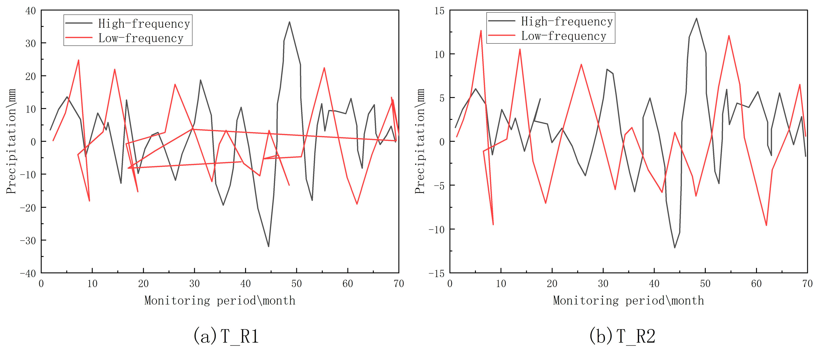
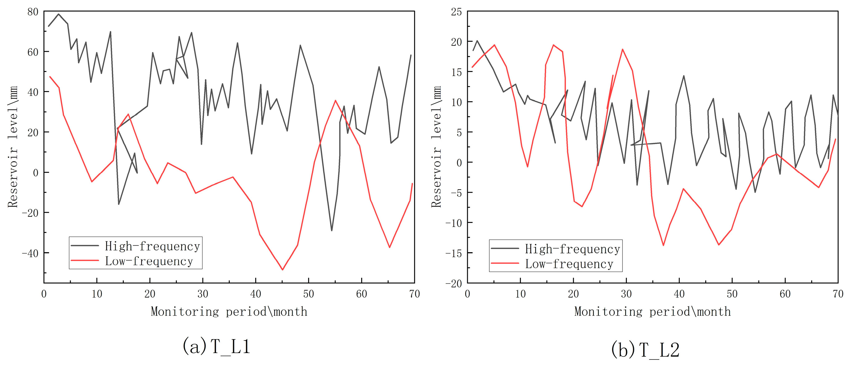
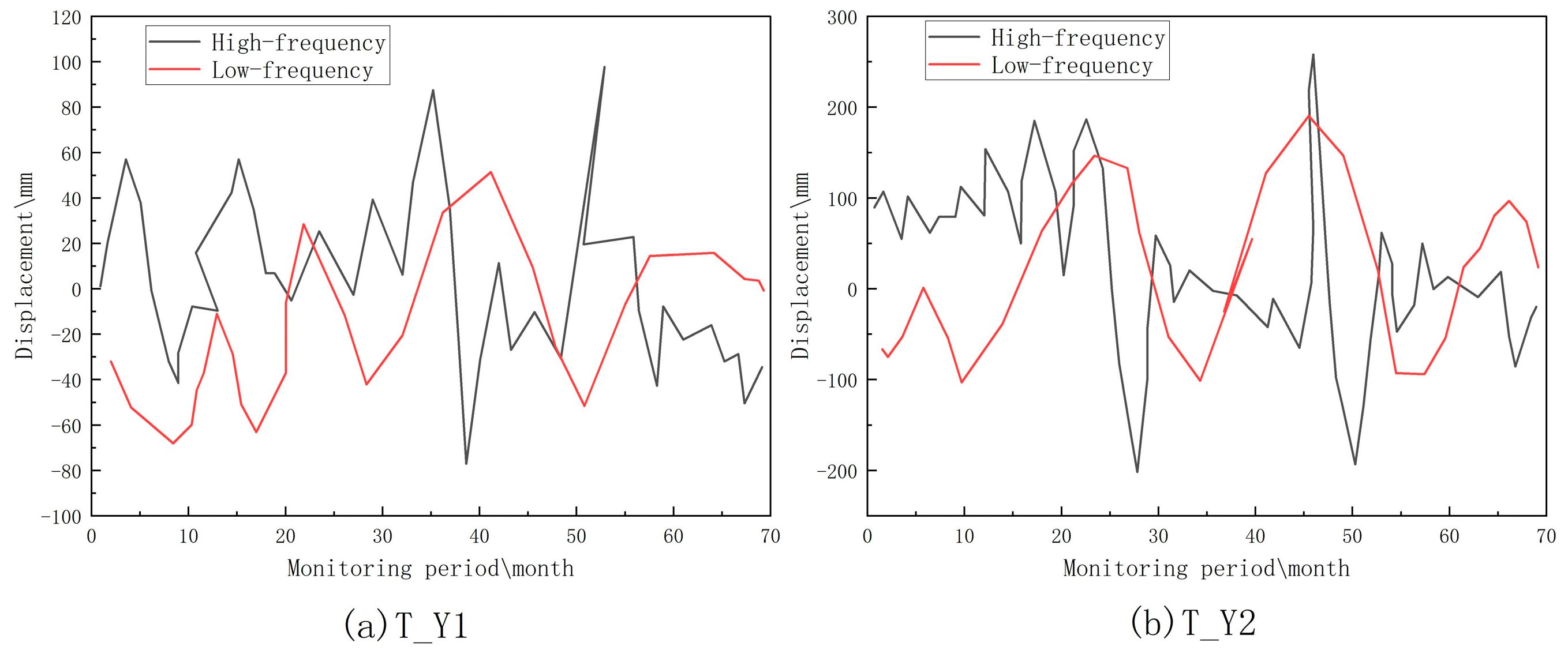
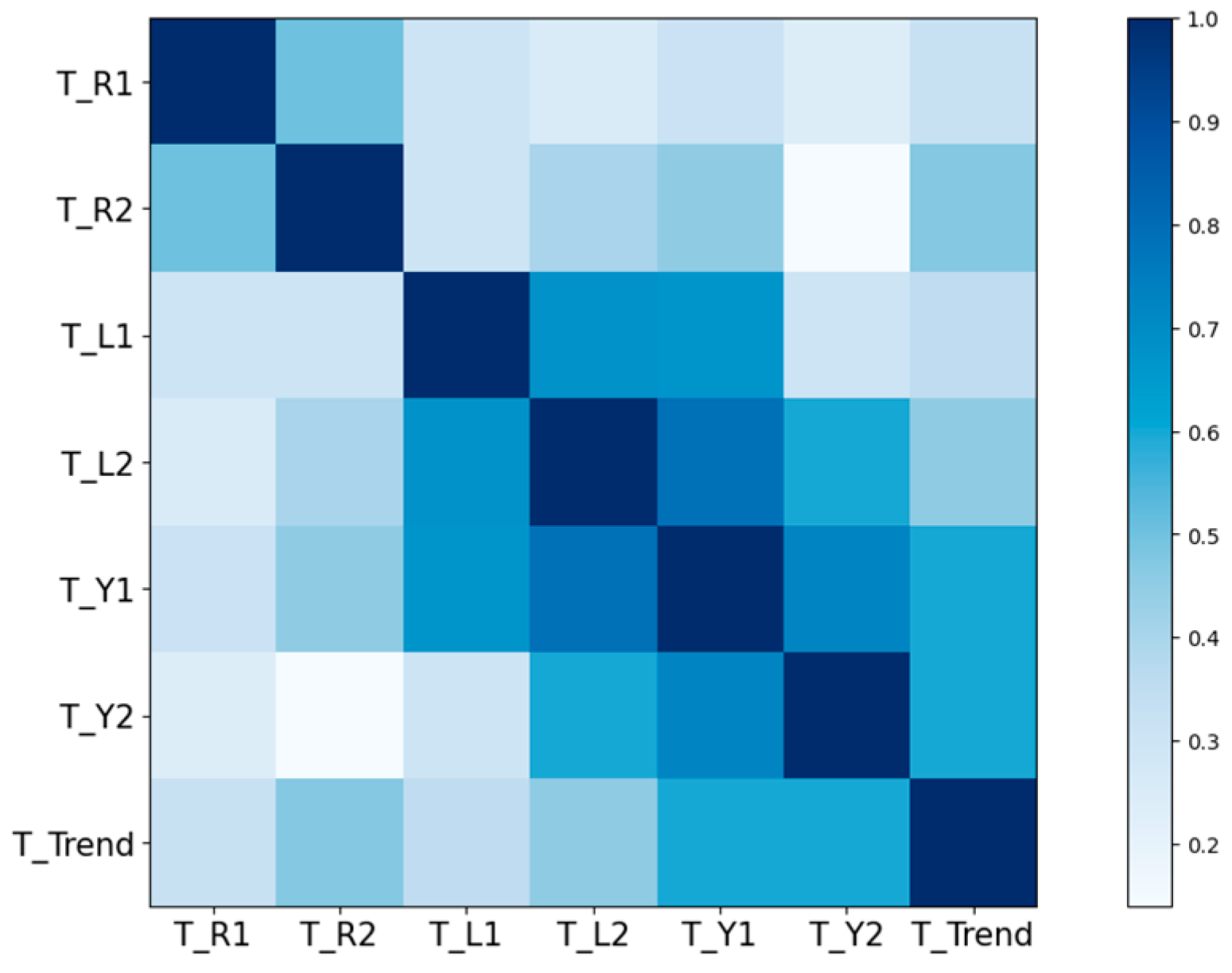
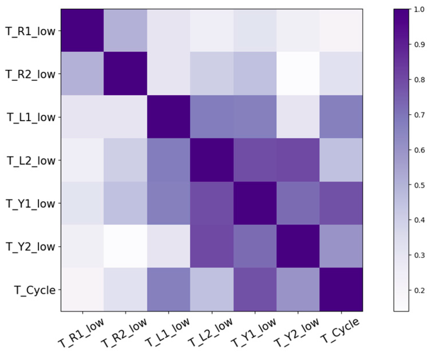
In order to dig into the correlation information between the influencing factors and landslide displacement, the trigger factor data are decomposed to obtain the high-frequency and low-frequency components, and $K$ = 2, $\alpha$ = 1858, $\lambda$ = 0.2 are set. The decomposition results are presented in Figure 16, Figure 17 and Figure 18. Subsequently, the Grey correlation between the high-frequency and low-frequency sequences with the components after the decomposition of the landslide displacements is calculated, as shown in Figure 19, Figure 20 and Figure 21, respectively.

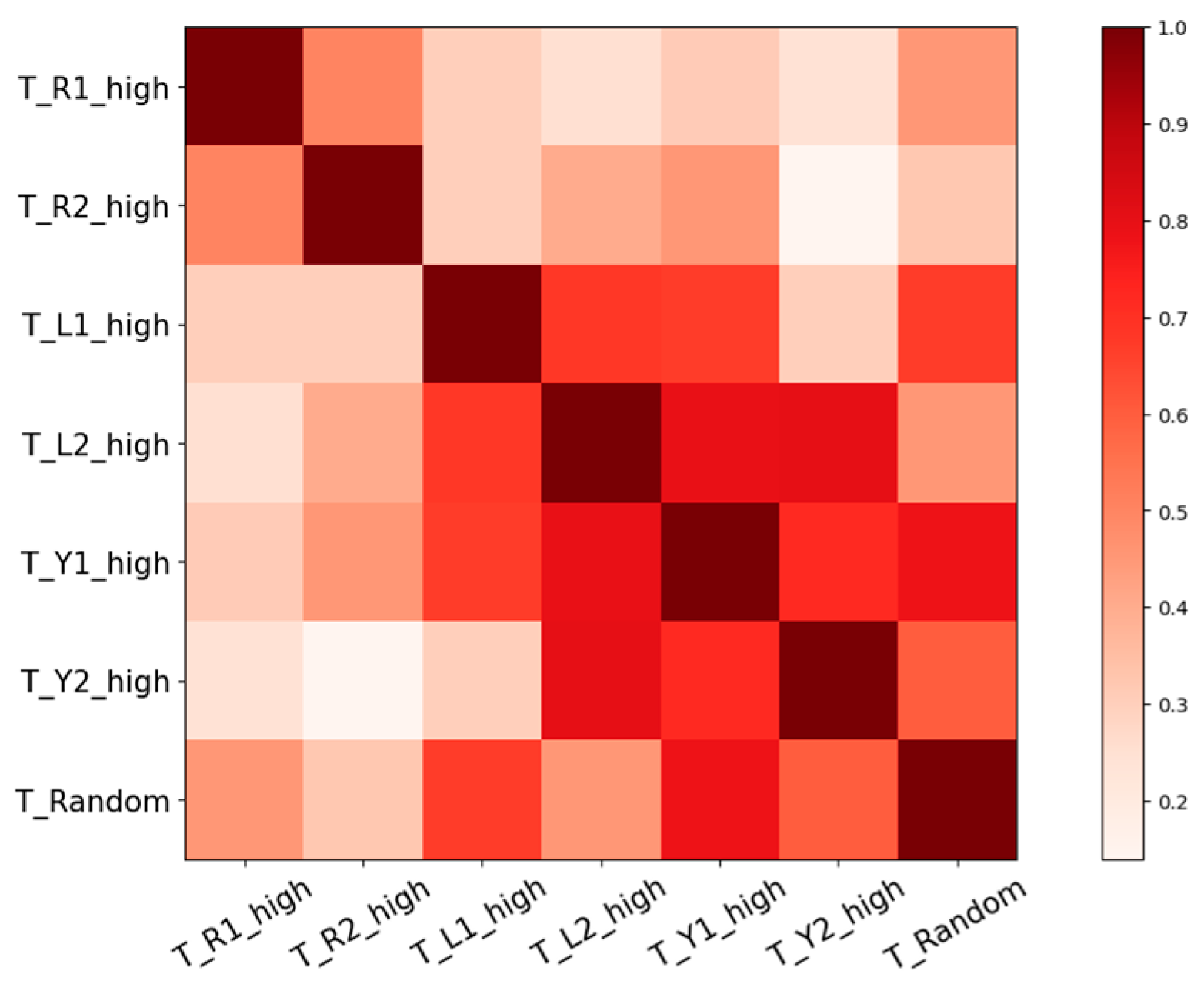
The optimized Variational Mode Decomposition (VMD) algorithm is utilized to decompose the sequence of triggering factors into high-frequency and low-frequency components. The low-frequency component exhibits discernible periodicity, with trend changes that evolve gradually over time. Conversely, the high-frequency component presents a more complex pattern, characterized by substantial and irregular fluctuations, which signify abrupt changes in the signal. Furthermore, the Grey correlation analysis (GRA) confusion matrix reveals a strong correlation close to 1 between the low-frequency trigger factors and the periodic term of displacement, as well as between the high-frequency trigger factors and the random term of displacement. This indicates that these trigger factors exhibit a significant influence on the corresponding displacement components. Consequently, it is essential to incorporate these highly correlated trigger factors into the prediction model for their respective displacement components, thereby enhancing the model’s accuracy and reliability.

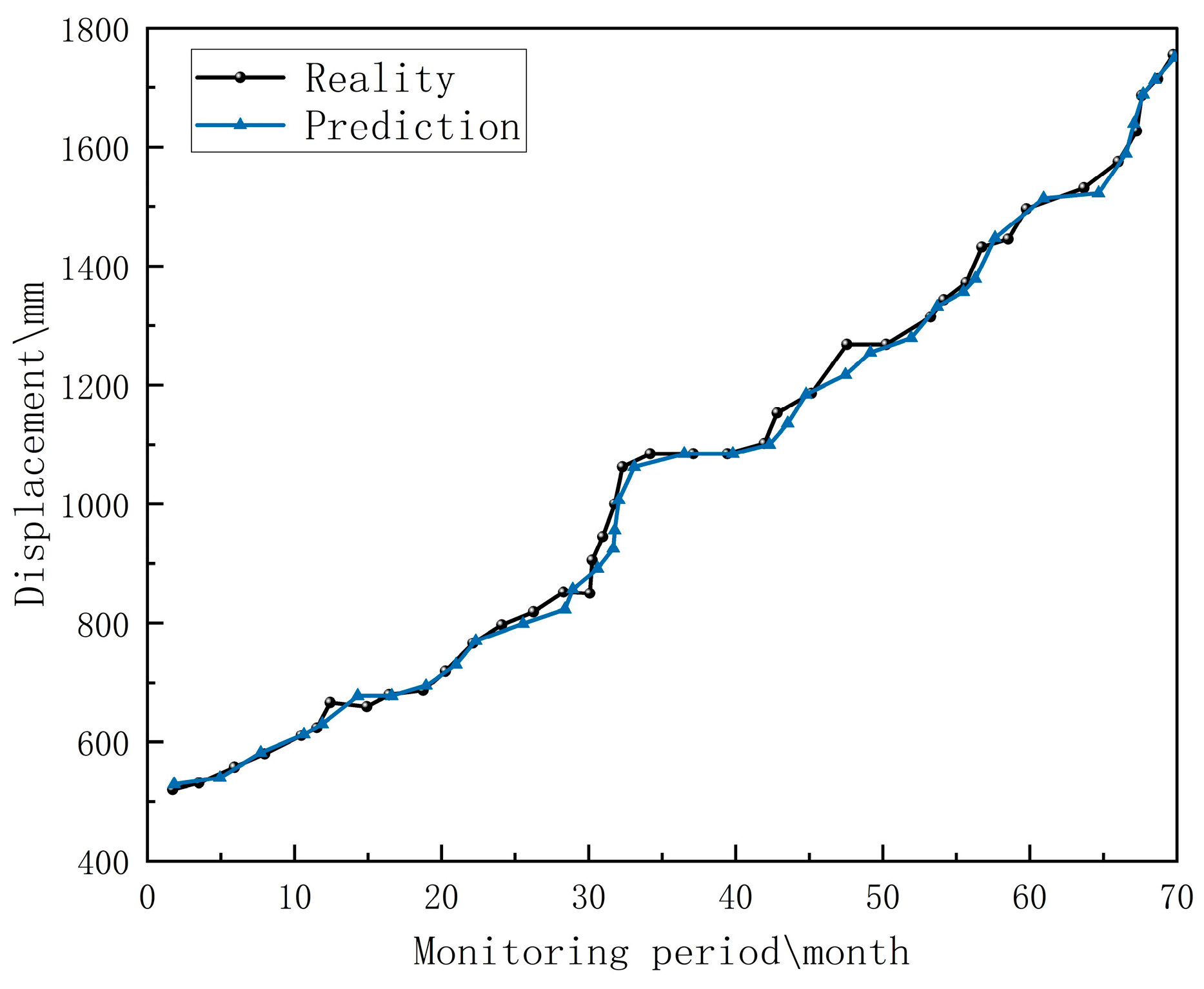
6.6.6. The Displacement Prediction Result of the Trend Term

The predicted displacements of the trend term exhibit a smooth curve over time, without considering the induced factors. The trend term displacement values of each monitoring point in the test set are used as inputs to the model to predict the trend term displacement values at the next time point. The results of the model prediction are depicted in Figure 22, illustrating that the model effectively captures the trend term displacement, and the predicted values closely align with the actual values.

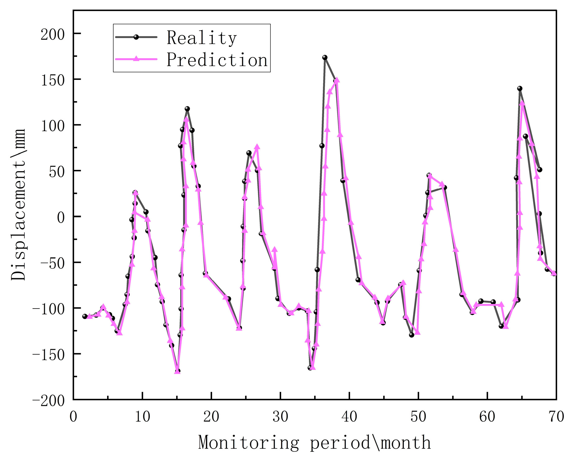
6.6.7. The Displacement Prediction Result of the Periodic Term

Based on the calculated correlation results between the cycle term displacement components and the inducing factors, it is determined that the low-frequency component of the first 40 months in the rainfall influencing factor of the eight gates exhibits the highest correlation with the cycle term displacement. Similarly, the low-frequency component of the average reservoir level in the reservoir level influencing factor has the highest correlation with the cycle term displacement. Consequently, $T_{-}R{2}_{-}low$ and $T_{-}L{2}_{-}low$ are identified as key inducing factors, forming a set of eigenvectors with the values of the cycle term displacements. These serve as inputs for predicting the cycle term displacements, and the prediction results are illustrated in Figure 23.

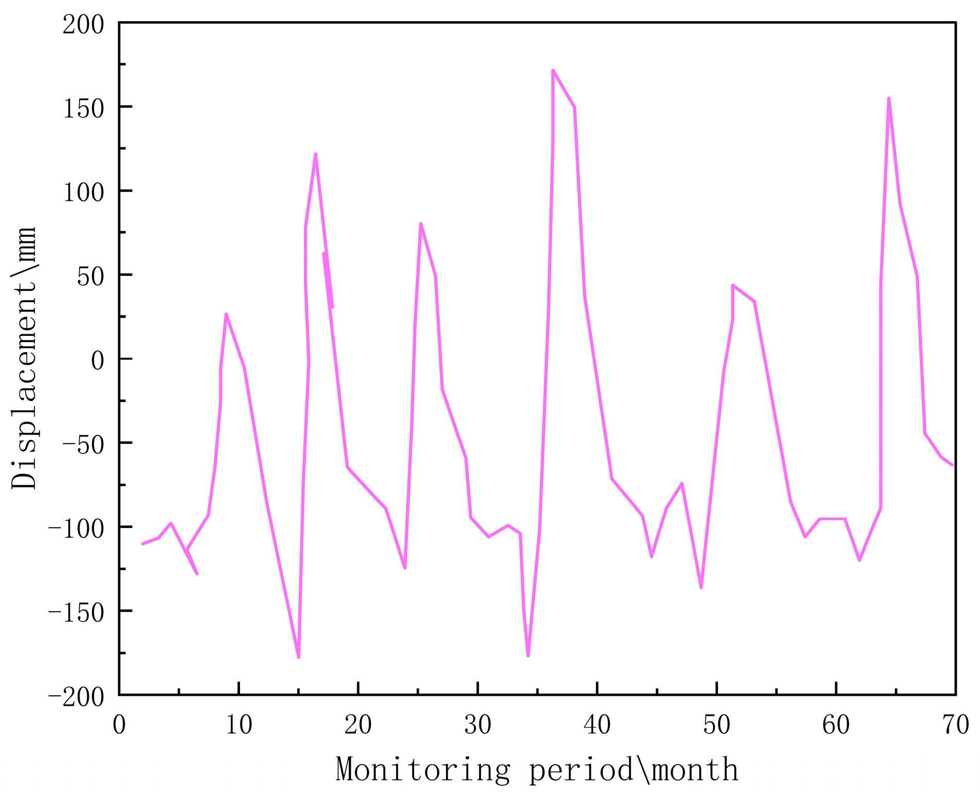
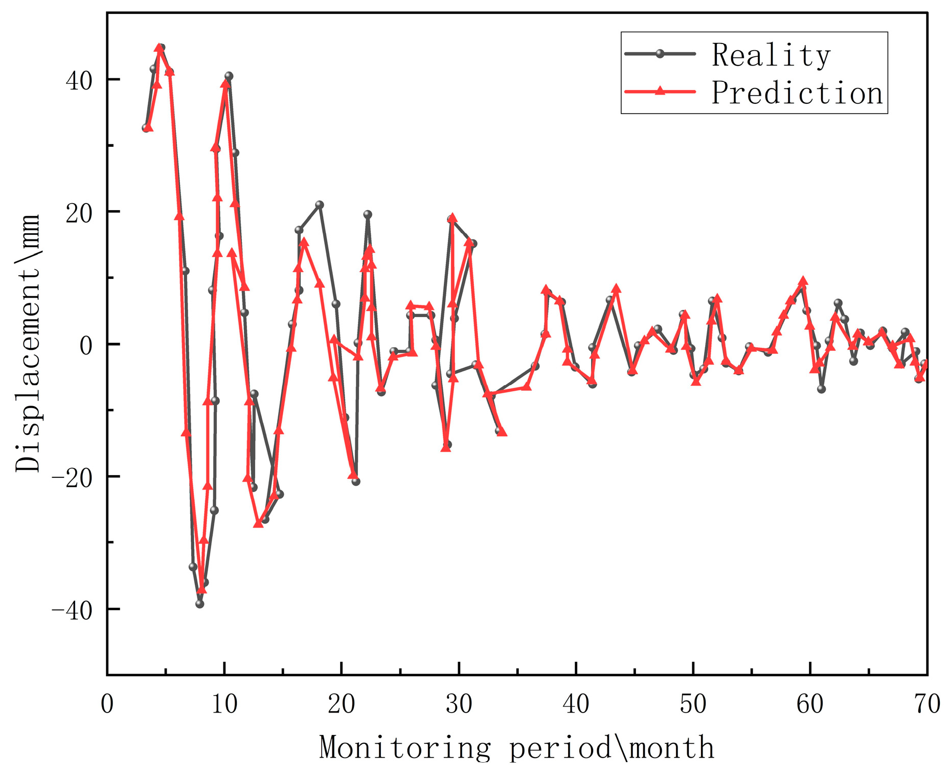
6.6.8. The Displacement Prediction Result of the Random Term

Based on the correlation results between the random term displacement components and the inducing factors, it is determined that the high-frequency component of the average rainfall among the rainfall influencing factors of the Bazimen landslide exhibits the highest correlation with the random term displacement. Similarly, the high-frequency component of the average borehole reservoir level among the reservoir level influencing factors has the highest correlation with the random term displacement. Consequently, $T_{-}R{1}_{-}high$ and $T_{-}L{2}_{-}high$ are identified as key inducing factors, forming a set of eigenvectors with the values of the random term displacement as inputs to the prediction model for forecasting the periodic term displacement. The prediction results are depicted in Figure 24.

Observational analysis indicates that the prediction error for random displacement components is notably higher than that for periodic term displacement components. This discrepancy can be attributed to the random displacement being subject to significant nonlinear fluctuations, which exhibit minimal regularity and present a more substantial challenge for precise fitting. Despite this, the model exhibits improved predictability around periods of sudden change in landslides, leading to an overall enhancement in prediction accuracy.

6.6.9. Comparative Analysis of Total Displacement Prediction Results

Utilizing the time series addition model of Equation (1), the overall displacement prediction is derived by superimposing the predictions of trend term, periodic term, and random term displacements. The prediction results are illustrated in Figure 25, demonstrating high prediction accuracy when comparing the predicted values with the actual observed values.

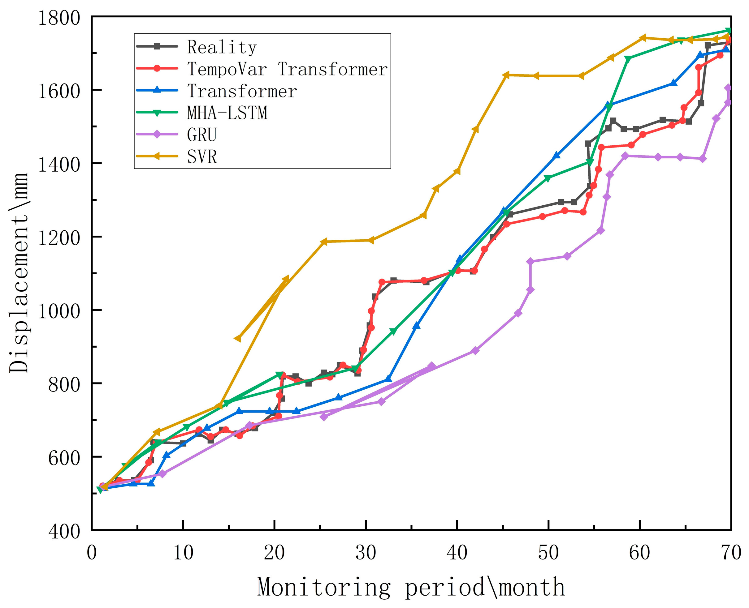
To validate that the proposed prediction model outperforms traditional methods and to ensure the consistency of the optimized VMD decomposition method, this paper compares the proposed model with the time-displacement sequence prediction models Transformer, MHA-LSTM, GRU, and SVR proposed by previous researchers. The results of the comparative experiments are presented in

Table 5. Comparison of the prediction errors of traditional displacement prediction models.

Prediction Model	Predictive Evaluation Value
	RMSE (mm)	MAPE (%)
SVR	16.72	21.67
GRU	14.07	16.92
MHA-LSTM	11.95	12.98
Transformer	6.08	6.32
TempoVar-Transformer	1.86	4.85

, and the prediction outcomes of various models are depicted in Figure 26, The REC curve of the TempoVar-Transformer prediction model is shown in Figure 27.

Observing the displacement time curves in Figure 24, it is evident that the predicted values obtained by the proposed model closely align with the trend and magnitude of the actual displacement values. Additionally, as indicated in Table 3, the root-mean-square error of the prediction model in this paper has been reduced by 69.4% compared to the best-performing previous model, and the Mean Absolute Percentage Error has reduced by 23.3%. These enhancements underscore a substantial improvement in prediction accuracy. In the REC curve diagram, “area” refers to the area under the curve (AUC), which is used to measure the classifier’s ability to distinguish between positive and negative samples. The value of “area” in the diagram (0.92) indicates that the prediction accuracy of landslide displacement is relatively high, possessing significant practical meaning.

Simultaneously, it is found that the obvious accelerated deformation of the Bazimen landslide usually occurs after rainfall, and the focus of the prediction model on rainfall events is consistent with the deformation law of the landslide.

Due to the model being tested only on a specific dataset, lacking credibility and generalization ability, this study will also compare predictions on two different monitoring points simultaneously on the training and test sets, providing compelling data to support the findings.

Table 6. Comparison of different monitoring points.

GPS Station	Model	Training Set		Testing Set
		RMSE (mm)	MAPE (%)	RMSE (mm)	MAPE (%)
ZG110	SVR	7.88	6.54	20.87	25.12
	GRU	3.25	5.09	19.76	17.34
	MHA-LSTM	4.42	7.92	16.53	18.79
	Transformer	2.89	3.34	14.32	11.92
	TempoVar-Transformer	1.56	2.69	5.77	8.67
ZG111	SVR	5.93	4.59	16.72	21.67
	GRU	3.91	4.32	14.07	16.92
	MHA-LSTM	3.76	6.64	11.95	12.98
	Transformer	2.40	2.01	6.08	6.32
	TempoVar-Transformer	0.91	1.88	1.86	4.85

shows that the composite prediction model proposed in this paper outperforms other models at both GPS monitoring points, with both groups exhibiting optimal performance. However, due to the relatively stable landslide data at the monitoring point ZG110 during some time periods, the change characteristics of the influencing factors are not obvious, resulting in a larger gap between the test and training data. This experiment demonstrates the model’s versatility across different locations, enhancing its generalizability and robustness beyond the specific case studies.

In summary, the proposed model excels in extracting topographic change information, with a particular emphasis on significant events such as displacement peaks and rainfall episodes. It adeptly captures the underlying patterns governing landslide displacement, aligning closely with geological principles. This adherence to geological laws instills high confidence in the model’s results, making it a robust tool for predicting and understanding landslide dynamics.

7. Discussion and Conclusions

In this paper, we have proposed a novel composite time series displacement prediction model, termed (GOA-GA-VMD)-GRA-(TempoVar-Transformer). This model delves into the evolutionary mechanisms underlying the dynamic interplay between landslide triggers and displacement. Building on the foundation of previous studies, we have improved the accuracy of our predictions [41]. Its versatility and applicability make it a promising tool for researchers.

• Our model harnesses a swarm intelligence coupling optimization algorithm to optimize the hyper-parameters of Variational Mode Decomposition (VMD) automatically. This algorithm leverages the synergistic benefits of diverse optimization methods, ensuring a decomposition effect of higher fidelity and enhancing the efficiency of the VMD process. This strategy not only improves the decomposition quality but also validates the prediction through a layered reconstruction of landslide displacement data.
• By analyzing the dynamic responses of landslides to various inducing factors, we have dismantled the sequence of these factors and conducted a quantitative Grey correlation degree evaluation. This evaluation, based on displacement components, accurately identifies the pivotal inducing factors. Consequently, we have established feature vector groups with varying scales as inputs for the subsequent prediction model. This approach effectively captures a range of time evolution characteristics and the effects of displacement deformation.
• The TempoVar-Transformer model introduced in this paper adeptly captures the dynamic temporal relationships between different trigger sequences within the same time step and across different time steps for the same trigger feature. This granular time-series modeling provides a comprehensive analysis of the evolutionary dynamics of landslide displacement, leading to more precise and reliable displacement predictions.
• Although the composite prediction model proposed in this paper has achieved satisfactory results on the existing landslide data, there are some shortcomings. The factors affecting landslides may lead to repetitions, omissions, and prediction delays. The model only considers the influence of rainfall and reservoir water level on landslide displacement separately, leading to repetitions in the intermediate effects. This is because a portion of the rainfall enters the reservoir through runoff, increasing the reservoir water level. This, in turn, results in increased errors and a lack of cohesion with the geographical significance of the landslide. Future research can enhance the precision of data analysis, combine geographical and physical knowledge to simulate the direct relationship model between rainfall and reservoir water level, and then apply it comprehensively to landslide prediction.
• Although the model proposed in this paper has high prediction accuracy, it is large in size, requires extensive training data, and has low computational efficiency. With the availability of more effective long-term time series data and stronger data processing algorithms in the future, this shortcoming can be avoided.

In conclusion, the prediction model still achieved good results. Building on the research presented in this paper, the predictive model can be integrated into existing landslide prediction systems to enable real-time monitoring of landslide activities. By issuing alerts in advance of potential displacements, the model can help reduce casualties and property damage. In urban planning and land use, the results of landslide displacement predictions can be used to avoid constructing important infrastructure and residential areas in high-risk zones, or to implement reinforcement measures to ensure safety. Continuous monitoring and data collection will assist researchers in further refining and optimizing the predictive model, enhancing its accuracy, and thereby providing more reliable support for long-term landslide prevention and management efforts.

References

1. Wu, W.; Guo, S.; Shao, Z. Landslide risk evaluation and its causative factors in typical mountain environment of China: A case study of Yunfu City. Ecol. Indic. 2023, 154, 110821. [Google Scholar] [CrossRef]
2. Tyagi, A.; Kamal Tiwari, R.; James, N. A review on spatial, temporal and magnitude prediction of landslide hazard. J. Asian Earth Sci. X 2022, 7, 100099. [Google Scholar] [CrossRef]
3. Tang, H.; Wasowski, J.; Juang, C.H. Geohazards in the three Gorges Reservoir Area, China—Lessons learned from decades of research. Eng. Geol. 2019, 261, 105267. [Google Scholar] [CrossRef]
4. Bednarik, M.; Yilmaz, I.; Marschalko, M. Landslide hazard and risk assessment: A case study from the Hlohovec–Sered’landslide area in south-west Slovakia. Nat. Hazards 2012, 64, 547–575. [Google Scholar] [CrossRef]
5. Zhang, Z.; Tan, Y.J.; Walter, F.; He, S.; Chmiel, M.; Su, J. Seismic monitoring and geomorphic impacts of the catastrophic 2018 Baige landslide hazard cascades in the Tibetan plateau. J. Geophys. Res. Earth Surf. 2024, 129, e2023JF007363. [Google Scholar] [CrossRef]
6. Li, C.; Criss, R.E.; Fu, Z.; Long, J.; Tan, Q. Evolution characteristics and displacement forecasting model of landslides with stair-step sliding surface along the Xiangxi River, three Gorges Reservoir region, China. Eng. Geol. 2021, 283, 105961. [Google Scholar] [CrossRef]
7. Nava, L.; Carraro, E.; Reyes-Carmona, C.; Puliero, S.; Bhuyan, K.; Rosi, A.; Monserrat, O.; Floris, M.; Meena, S.R.; Galve, J.P.; et al. Landslide displacement forecasting using deep learning and monitoring data across selected sites. Landslides 2023, 20, 2111–2129. [Google Scholar] [CrossRef]
8. Xiang, X.; Xiao, J.; Wen, H.; Li, Z.; Huang, J. Prediction of landslide step-like displacement using factor preprocessing-based hybrid optimized SVR model in the Three Gorges Reservoir, China. Gondwana Res. 2024, 126, 289–304. [Google Scholar] [CrossRef]
9. Yang, W. Landslide Displacement Prediction Based on VMD-LSTM-GM Model Considering Rainfall. In China Satellite Navigation Conference (CSNC 2022): Volume I; Springer Nature: Berlin/Heidelberg, Germany, 2022; Volume 908, p. 34. [Google Scholar]
10. Guo, Z.; Chen, L.; Gui, L.; Du, J.; Yin, K.; Do, H.M. Landslide displacement prediction based on variational mode decomposition and WA-GWO-BP model. Landslides 2020, 17, 567–583. [Google Scholar] [CrossRef]
11. Xing, Y.; Yue, J.; Chen, C.; Cong, K.; Zhu, S.; Bian, Y. Dynamic displacement forecasting of dashuitian landslide in China using variational mode decomposition and stack long short-term memory network. Appl. Sci. 2019, 9, 2951. [Google Scholar] [CrossRef]
12. Liu, B.; Liu, C.; Zhou, Y.; Wang, D. A chatter detection method in milling based on gray wolf optimization VMD and multi-entropy features. Int. J. Adv. Manuf. Technol. 2023, 125, 831–854. [Google Scholar] [CrossRef]
13. Liu, T.; Wang, Y.; Cui, L.; Zhang, C. Study on Fault Diagnosis Method of Key Components of the Gearbox Under Variable Working Conditions Based on Improved VMD Algorithm. In International Conference on the Efficiency and Performance Engineering Network; Springer: Cham, Switzerland, 2022; pp. 74–89. [Google Scholar]
14. Guan, S.; Zhu, Y.; Zhou, L.; Deng, H.; Luo, X. Prediction of Landslide Displacement Using EMD-PSO-ELM with Multiple Factors. In Proceedings of the 2018 7th International Conference on Digital Home (ICDH), Guilin, China, 30 November–1 December 2018; pp. 230–235. [Google Scholar] [CrossRef]
15. Cai, Z.; Xu, W.; Meng, Y.; Shi, C.; Wang, R. Prediction of landslide displacement based on GA-LSSVM with multiple factors. Bull. Eng. Geol. Environ. 2016, 75, 637–646. [Google Scholar] [CrossRef]
16. Sahoo, A.; Ghose, D.K. Flood Forecasting Using Hybrid SVM-GOA Model: A Case Study. In Intelligent Systems: Proceedings of ICMIB 2021; Springer: Singapore, 2022; pp. 407–416. [Google Scholar]
17. Lin, Z.; Sun, X.; Ji, Y. Landslide Displacement Prediction Model Using Time Series Analysis Method and Modified LSTM Model. Electronics 2022, 11, 1519. [Google Scholar] [CrossRef]
18. Pham, B.T.; Tien Bui, D.; Pourghasemi, H.R.; Indra, P.; Dholakia, M. Landslide susceptibility assesssment in the Uttarakhand area (India) using GIS: A comparison study of prediction capability of naïve bayes, multilayer perceptron neural networks, and functional trees methods. Theor. Appl. Climatol. 2017, 128, 255–273. [Google Scholar] [CrossRef]
19. Zheng, T.; Zhao, Q.H.; Hu, J.B.; Jiang, J.F.; Su, R. An IPSO-RNN machine learning model for soil landslide displacement prediction. Arab. J. Geosci. 2021, 14, 1191. [Google Scholar] [CrossRef]
20. Yang, B.; Yin, K.; Lacasse, S.; Liu, Z. Time series analysis and long short-term memory neural network to predict landslide displacement. Landslides 2019, 16, 677–694. [Google Scholar] [CrossRef]
21. Jiang, P.; Chen, J.; Zeng, Z. Multi Step Prediction of Landslide Displacement Time Series Based on Extended Kalman Filter and Back Propagation Trough Time. In Advances in Neural Networks–ISNN 2019: 16th International Symposium on Neural Networks, ISNN 2019, Moscow, Russia, 10–12 July 2019, Proceedings, Part I 16; Springer: Berlin/Heidelberg, Germany, 2019; pp. 184–193. [Google Scholar]
22. Liu, Z.; Ma, J.; Xia, D.; Jiang, S.; Ren, Z.; Tan, C.; Guo, H. Toward the reliable prediction of reservoir landslide displacement using earthworm optimization algorithm-optimized support vector regression (EOA-SVR). Nat. Hazards 2023, 120, 3165–3188. [Google Scholar] [CrossRef]
23. Li, L.M.; Zhang, M.Y.; Wen, Z.Z. Dynamic prediction of landslide displacement using singular spectrum analysis and stack long short-term memory network. J. Mt. Sci. 2021, 18, 2597–2611. [Google Scholar] [CrossRef]
24. Meng, Y.; Qin, Y.; Cai, Z.; Tian, B.; Yuan, C.; Zhang, X.; Zuo, Q. Dynamic forecast model for landslide displacement with step-like deformation by applying GRU with EMD and error correction. Bull. Eng. Geol. Environ. 2023, 82, 211. [Google Scholar] [CrossRef]
25. Wang, J.; Nie, G.; Xue, C. Landslide displacement prediction based on time series analysis and data assimilation with hydrological factors. Arab. J. Geosci. 2020, 13, 460. [Google Scholar] [CrossRef]
26. Wang, L.; Chen, Y.; Huang, X.; Zhang, L.; Li, X.; Wang, S. Displacement prediction method of rainfall-induced landslide considering multiple influencing factors. Nat. Hazards 2023, 115, 1051–1069. [Google Scholar] [CrossRef]
27. Bai, D.; Lu, G.; Zhu, Z.; Tang, J.; Fang, J.; Wen, A. Using time series analysis and dual-stage attention-based recurrent neural network to predict landslide displacement. Environ. Earth Sci. 2022, 81, 509. [Google Scholar] [CrossRef]
28. Cai, B.; Huang, G.; Yang, S.; Xiang, Y.; Chi, C.H. SE-shapelets: Semi-supervised Clustering of Time Series Using Representative Shapelets. Expert Syst. Appl. 2024, 240, 122584. [Google Scholar] [CrossRef]
29. Ahmadi, F.; Tohidi, M.; Sadrianzade, M. Streamflow prediction using a hybrid methodology based on variational mode decomposition (VMD) and machine learning approaches. Appl. Water Sci. 2023, 13, 135. [Google Scholar] [CrossRef]
30. Li, L.; Meng, W.; Liu, X.; Fei, J. Research on Rolling Bearing Fault Diagnosis Based on Variational Modal Decomposition Parameter Optimization and an Improved Support Vector Machine. Electronics 2023, 12, 1290. [Google Scholar] [CrossRef]
31. CH, S.; P, V. Ameliorate grasshopper optimization algorithm based long short term memory classification for face emotion recognition system. Multimed. Tools Appl. 2023, 1–18. [Google Scholar] [CrossRef]
32. Mbamba, C.K.; Batstone, D.J. Optimization of deep learning models for forecasting performance in the water industry using genetic algorithms. Comput. Chem. Eng. 2023, 175, 108276. [Google Scholar] [CrossRef]
33. Goudarzi, S.; Hassan, W.H.; Anisi, M.H.; Soleymani, S.A. Comparison between hybridized algorithm of GA–SA and ABC, GA, DE and PSO for vertical-handover in heterogeneous wireless networks. Sādhanā 2016, 41, 727–753. [Google Scholar] [CrossRef]
34. Ali, S.F.; Bhattacharjee, B.; Rakshit, D. Grasshopper Optimization Algorithm vis-a-vis Genetic Algorithm for Energy Optimization in Conditioned Buildings with Varying Hours of Occupancy in Composite Climate of Delhi. In International Conference on Building Energy and Environment; Springer: Singapore, 2022; pp. 1267–1278. [Google Scholar]
35. Liu, Y.; Huang, X.; Duan, J.; Zhang, H. The assessment of traffic accident risk based on grey relational analysis and fuzzy comprehensive evaluation method. Nat. Hazards 2017, 88, 1409–1422. [Google Scholar] [CrossRef]
36. Vaswani, A.; Shazeer, N.; Parmar, N.; Uszkoreit, J.; Jones, L.; Gomez, A.N.; Kaiser, Ł.; Polosukhin, I. Attention is all you need. Adv. Neural Inf. Process. Syst. 2017, 30, 5998–6008. [Google Scholar]
37. Tomás, R.; Li, Z.; Liu, P.; Singleton, A.; Hoey, T.; Cheng, X. Spatiotemporal characteristics of the Huangtupo landslide in the Three Gorges region (China) constrained by radar interferometry. Geophys. J. Int. 2014, 197, 213–232. [Google Scholar] [CrossRef]
38. Jiao, Y.-Y.; Zhang, H.-Q.; Tang, H.-M.; Zhang, X.-L.; Adoko, A.C.; Tian, H.-N. Simulating the process of reservoir-impoundment-induced landslide using the extended DDA method. Eng. Geol. 2014, 182, 37–48. [Google Scholar] [CrossRef]
39. Remondo, J.; Bonachea, J.; Rivas, V.; Sánchez-Espeso, J.; Bruschi, V.; Cendrero, A.; de Terán, J.R.D.; Fernández-Maroto, G.; Gómez-Arozamena, J.; González-Díez, A.; et al. Landslide hazard scenarios based on both past landslides and precipitation. In Advancing Culture of Living with Landslides: Volume 2 Advances in Landslide Science; Springer: Berlin/Heidelberg, Germany, 2017; pp. 981–988. [Google Scholar]
40. Han, H.; Shi, B.; Zhang, L. Prediction of landslide sharp increase displacement by SVM with considering hysteresis of groundwater change. Eng. Geol. 2021, 280, 105876. [Google Scholar] [CrossRef]
41. Zhou, C.; Yin, K.; Cao, Y.; Ahmed, B. Application of time series analysis and PSO–SVM model in predicting the Bazimen landslide in the Three Gorges Reservoir, China. Eng. Geol. 2016, 204, 108–120. [Google Scholar] [CrossRef]
Figure 1. The overall frame diagram of the landslide displacement prediction model.
Electronics 13 01271 g001
Figure 2. Schematic diagram of GA initialization code.
Electronics 13 01271 g002
Figure 3. Schematic diagram of GOA-GA swarm algorithm optimization.
Electronics 13 01271 g003
Figure 4. Flowchart of the displacement decomposition of the GOA-GA-VMD combination.
Electronics 13 01271 g004
Figure 5. Schematic diagram of the time series variable analysis module.
Electronics 13 01271 g005
Figure 6. TempoVar-Transformer algorithm model architecture.
Electronics 13 01271 g006
Figure 7. Satellite picture of the Bazimen landslide.
Electronics 13 01271 g007
Figure 8. Planar Contour Map of the Bazimen Landslide.
Electronics 13 01271 g008
Figure 9. Time-displacement rainfall-reservoir level curve of the monitoring point of the Bazimen landslide.
Electronics 13 01271 g009
Figure 10. Plot of observed total displacement.
Electronics 13 01271 g010
Figure 11. Displacement profile of trend term after decomposition.
Electronics 13 01271 g011
Figure 12. Displacement profile of the periodic term after decomposition.
Electronics 13 01271 g012
Figure 13. Displacement profile of the random term after decomposition.
Electronics 13 01271 g013
Figure 14. The Impact of Parameters Optimized by Different Optimization Algorithms on the Decomposition Effect. The blue bars represent the optimized parameter values of the optimization algorithm, corresponding to the left y-axis; the green bars represent the decomposition loss of the hyperparameters obtained by the optimization algorithm for VMD.
Electronics 13 01271 g014
Figure 15. Correlation diagram between landslide displacement and quantitative analysis of influencing factors.
Electronics 13 01271 g015
Figure 16. Plot of high and low frequency decomposition of rainfall factors.
Electronics 13 01271 g016
Figure 17. Pore pressure factor high and low frequency decomposition plots.
Electronics 13 01271 g017
Figure 18. High and low frequency decomposition of observed displacements.
Electronics 13 01271 g018
Figure 19. Grey correlation of displacement trend components with high-frequency features.
Electronics 13 01271 g019
Figure 20. Grey correlation of displacement period components with low-frequency features.
Electronics 13 01271 g020
Figure 21. Grey correlation of displacement random components with high-frequency features.
Electronics 13 01271 g021
Figure 22. Trend term displacement projections.
Electronics 13 01271 g022
Figure 23. Periodic term displacement projections.
Electronics 13 01271 g023
Figure 24. Random term displacement prediction results.
Electronics 13 01271 g024
Figure 25. Total displacement prediction results.
Electronics 13 01271 g025
Figure 26. Comparison of the effects of different prediction methods.
Electronics 13 01271 g026
Figure 27. REC curve consisting of displacement observations and predicted values from the TemporVar-Transformer model.
Electronics 13 01271 g027