A Novel Distributed Adaptive Controller for Multi-Agent Systems with Double-Integrator Dynamics: A Hedging-Based Approach

Abstract

In this paper, we focus on designing a model reference adaptive control-based distributed control law to drive a set of agents with double-integrator dynamics in a leader–follower fashion in the presence of system anomalies such as agent-based uncertainties, unknown control effectiveness, and actuator dynamics. In particular, we introduce a novel hedging-based reference model with second-order dynamics to allow an adaptation in the presence of actuator dynamics. We show the stability of the overall closed-loop multi-agent system by utilizing the Lyapunov Stability Theory, where we analyze the stability condition by using the Linear Matrix Inequalities method to show the boundedness of the reference model and actuator states. Finally, we illustrate the efficacy of the proposed distributed adaptive controller on an undirected and connected line graph in five cases.

1. Introduction

Thanks to the gradually increasing efficiency of off-shelf electro-mechanical components and recent advances in robust algorithms, multi-agent systems create highly promising opportunities to complete complex tasks using several low-level agents instead of just one high-level and non-replaceable platform. Together with many others, new mission definitions and capabilities in aerospace (e.g., swarm aerial vehicles and satellite formations), ground (e.g., automated agriculture), and marine (e.g., patrol boats) are being developed by researchers and engineers in both academia and industry.

In the literature, many algorithms exist to provide collaborative behavior with multiple robots [1,2,3,4,5,6]. Note that consensus-based approaches are one of the superior approaches due to reduced network usage, simplicity in application, and experimentally validated results [7]. Researchers studied consensus-based approaches for systems with scalar dynamics [8,9,10,11], second-order dynamics [12,13,14,15], or systems with non-holonomic constraints [16,17,18,19] to provide a variety of purposes, such as consensus, leader–follower, and formation control. On the one hand, the analysis in [20] studies the behavior of distributed Riccati recursions for a multi-agent system, providing the required conditions for their convergence to a singular set of stabilizing matrices. Specifically, the class of algebraic Riccati equations is considered such that their results can be generalized for a wide range of control purposes. On the other hand, in [21], the authors studied the conditions for designing static distributed controllers for deterministic and stochastic systems. These conditions are then translated into an optimization problem to quantify the closeness of the designed distributed control systems. Note that none of the above papers are designed to suppress the effect of system anomalies.

Considering ideal multi-agent systems, classical control algorithms work with high performance in the absence of system anomalies. However, real physical systems are not ideal and are affected by different types of anomalies due to their nature. In the scope of this research, we collect these anomalies as uncertainty, unknown control effectiveness, and actuator dynamics. Hence, controllers designed in the studies referenced above cannot obtain control algorithms that provide stability guarantees and satisfactory transient responses in the presence of uncertainty and actuator dynamics, as well as unknown actuation inefficiencies. To guarantee overall stability, the researchers in [22,23,24,25,26,27] provide adaptive control of multi-agent systems with single-integrator dynamics subject to suppress the undesired effects of such anomalies. Note that multi-agent systems with single-integrator dynamics may not fully represent the real physical systems since most of them have higher-order (i.e., double-integrator) dynamics. Moreover, using single-integrator dynamics yields unsatisfactory and mostly oscillatory performance, which can be seen in the recent experimental results provided in [28]. The main reason for this is the absence of internal damping, together with a limited control authority for the single-integrator control system. In addition, the single-integrator system has a limited dynamic response (i.e., slower response to any change) that yields limited tracking response, lack of robustness, and less design flexibility.

To this end, one of the latest research results in [29] provides leader–follower-based integral sliding-mode control for multi-agent systems with nonlinear double-integrator dynamics in the presence of uncertain parameters and external disturbances with unknown upper bounds. Since upper bounds on disturbances are unknown in most of the practical applications, they improve existing controllers in an adaptive scheme to provide robustness. However, their study does not cover actuator dynamics and actuation efficiency problems. In [30,31], the high-order multi-agent system with uncertainty and actuator dynamics is controlled by utilizing distributed adaptive controllers. In addition, neither [30] nor [31] consider if the actuator effectiveness is unknown. Moreover, Refs. [30,31] require integral state vector usage in their control design. This approach can cause a slow response/update such that the control response cannot be updated directly. In addition, when an integral state approach is applied to a system, it requires some time for the integral terms to accumulate and reach a significant value, which may cause a poor transient response such as oscillations. Also, robustness issues may exist since integral terms can amplify high-frequency noise or measurement errors between the output of the agents and the reference command, which can even yield instability.

Hence, there is a fundamental gap in the analysis of distributed controllers on the uncertain multi-agent system in the presence of unknown control effectiveness and actuator dynamics. To close this gap and therefore improve the performance of the distributed adaptive control algorithms on real physical systems with such anomalies, in this paper, we design a distributed adaptive controller for double-integrator systems (that can be easily extended for higher-orders such as acceleration, jerk, and so on). This extension enables us to increase transient performance, obtain a faster response, and decrease required minimum actuator bandwidths for agents that increase the overall robustness of the system. This is due to the fact that the proposed controller does not require additional distributed signals that need to be integrated when you compare with current related results [30,31]. Note that the additional integrated distributed signals result in a slow response, a poor transient response, or a non-robust behavior in an overall multi-agent system. To summarize, in this paper, there are four main contributions to the literature in particular:

(1)

Designing a novel distributed adaptive control algorithm and a novel hedging-based reference model for multi-agent systems with double-integrator dynamics that uses position and velocities in the control law, which highly increases transient performance since it yields a faster update and enlarges the feasible actuator bandwidth set that increases the overall system performance and robustness.

(2)

Provides the first result for distributed adaptive control with double-integrator type multi-agent systems to deal with uncertainty, unknown control effectiveness, and actuator dynamics altogether. The proposed controller also yields a faster response, and hence, better performance while providing a level of robustness due to not needing a distributed signal integration. To show these advantages, we compare our performance results with the control algorithm developed in [31] in Section 4 of this paper.

(3)

Utilizing a compact form for both system dynamics and controller for all agents for investigating stability via Lyapunov Stability Theory and Linear Matrix Inequalities. This compact form enables extending controller design and stability analysis for systems with even higher than second-order dynamics (which can include acceleration, jerk, etc.) without any changes in Lyapunov-based stability analysis. For detailed information on this item, please see Remark 3 in Section 3.

(4)

Avoiding one of the assumptions that current high-order multi-agent distributed adaptive control literature is required for the boundedness of the reference model (see, for example, Assumption 3.1. of [31]).

The outline of this paper is as follows. In Section 2, we provide the general notation that is used in this paper and provide mathematical preliminaries on Graph Theory together with the definition and properties of the Projection operator. In Section 3, we provide dynamical equations for a multi-agent system with double-integrator dynamics in the presence of uncertainty, unknown control effectiveness, and actuator dynamics. We then introduce the novel hedging-based reference model with double-integrator dynamics to allow an adaptation that is not affected by the actuator dynamics. We design a novel distributed adaptive control law that enables tracking of the reference model even though the aforementioned system anomalies exist. We end this section by investigating the stability result of the overall closed-loop multi-agent system via Lyapunov Stability Theory and show the boundedness of the reference model and actuator dynamics by utilizing Linear Matrix Inequalities. In Section 4, we illustrate the performance of the designed controller with five cases for an undirected and connected line graph in a leader–follower setting. Finally, in Section 5, we summarize the results presented in the paper and mention future research directions.

2. Notation and Mathematical Preliminaries

The general notation of this paper can be seen in

Table 1. Notation.

${\mathbb{R}}_{-}$	Set of negative definite real numbers.
${\mathbb{R}}_{+}$	Set of positive definite real numbers.
$\mathbb{R}$	Set of real numbers.
${\mathbb{R}}^n$	Set of $n\times 1$ real column vectors.
${\mathbb{R}}_{+}^{n\times n}$	Set of $n\times n$ positive definite real matrices.
${\overline{\mathbb{R}}}_{+}^{n\times n}$	Set of $n\times n$ nonnegative definite real matrices.
${\mathbb{D}}^{n\times n}$	Set of $n\times n$ diagonal matrices.
${\mathbb{D}}_{+}^{n\times n}$	Set of $n\times n$ positive definite diagonal matrices.
${(·)}^{\mathrm{T}}$	Transpose of a matrix.
${(·)}^{-1}$	Inverse of a matrix.
$I_{n\times n}$	$n\times n$ identity matrix.
$0_n$	$n\times 1$ zero vector.
${\mathbf{1}}_n$	$n\times 1$ vector with all entries are 1.
Proj	Projection operator.
diag(·)	Diagonalized vector.
≜	Equality from the definition.
${\mathrm{col}}_i(·)$	ith column operator.

. In addition, since we utilize Graph Theory, for the results of this paper, we start with defining graph-theoretical notations that are standard in the literature [5]. In particular, for an undirected graph $\mathcal{G}$, which includes a set ${\mathcal{V}}_{\mathcal{G}}=\{1,\dots ,n\}$ of nodes and a set ${\mathcal{E}}_{\mathcal{G}}\subset {\mathcal{V}}_{\mathcal{G}}\times {\mathcal{V}}_{\mathcal{G}}$ of edges, nodes i and j are said to be neighbors if $(i,j)\in {\mathcal{E}}_{\mathcal{G}}$, which is denoted by with $i\sim j$. Each node’s degree is the number of neighbors of the regarding node. In other words, for a node i with degree $d_i$, the degree matrix of a graph $\mathcal{G}$ can be given by a diagonalized matrix of number of neighbors denoted by $\mathcal{D}\left(\mathcal{G}\right)\triangleq \mathrm{diag}(d_1,\dots ,d_n)\in {\mathbb{D}}^{n\times n}$. Regarding the definition of a path, a graph $\mathcal{G}$ is said to be connected if there is a path, $i_0{i}_1\cdots i_L$, that is a finite sequence of nodes between two consecutive nodes $i_{k-1}\sim i$ where $k=1,\dots ,L$ between any pair of distinct nodes. For a graph $\mathcal{G}$, the adjacency matrix $\mathcal{A}\left(\mathcal{G}\right)\in {\mathbb{D}}^{n\times n}$ is the matrix that represents the neighbors’ relation of agent i, where its elements are $\mathcal{A}{\left[\left(\mathcal{G}\right)\right]}_{ij}=1$ if the i’th and j’th nodes are neighbors, and, if not, $\mathcal{A}{\left[\left(\mathcal{G}\right)\right]}_{ij}=0$.

In addition, the Laplacian matrix of the graph $\mathcal{G}$, $\mathcal{L}\left(\mathcal{G}\right)\in {\overline{\mathbb{R}}}_{+}^{n\times n}$ is the main tool to represent the network characteristics of a graph based on the graph-theoretic approach. The relation for the Laplacian matrix is given by $\mathcal{L}\left(\mathcal{G}\right)\triangleq \mathcal{D}\left(\mathcal{G}\right)-\mathcal{A}\left(\mathcal{G}\right)$, and, for an undirected and connected graph, the spectrum of this Laplacian matrix $\mathcal{G}$ is ordered as $0={\lambda }_1\left(\mathcal{L}\left(\mathcal{G}\right)\right)<{\lambda }_2\left(\mathcal{L}\left(\mathcal{G}\right)\right)\le \dots \le {\lambda }_n\left(\mathcal{L}\left(\mathcal{G}\right)\right)$. Also, ${\mathbf{1}}_n$ is the eigenvector corresponding to the zero eigenvalue ${\lambda }_1\left(\mathcal{L}\left(\mathcal{G}\right)\right)$ satisfying $\left(\mathcal{L}\left(\mathcal{G}\right)\right){\mathbf{1}}_n=0_n$, as referenced in [5,32]. We note that, in this paper, the proposed approach is based on a leader–follower setting. For this purpose, we provide the following lemma.

Lemma 1.

Let $\mathcal{K}=\mathrm{diag}\left([k_1,\dots ,k_n]\right)\in {\mathbb{D}}^{n\times n}$ with $k_i\in \{0,1\}$, where $k_i=1$ for a leader agent(s) and $k_i=0$ for follower agent(s), for all $i=1,\dots ,n$, and assume that at least one element $k_i$ is nonzero. Then, for the Laplacian of a connected, undirected graph, $\mathcal{F}\left(\mathcal{G}\right)\triangleq \mathcal{L}\left(\mathcal{G}\right)+\mathcal{K}\in {\mathbb{R}}_{+}^{n\times n}$ [5].

In addition, the Projection operator is utilized for the adaptive update laws in the distributed adaptive controller designed in this paper. Specifically, $\mathrm{Proj}:\mathbb{R}\times \mathbb{R}\to \mathbb{R}$ with $y\in \mathbb{R}$ is utilized in adaptive update laws (8) and (9) as

$$\begin{array}{c}\hfill \mathrm{Proj}(\theta ,y)\left\{\begin{array}{cc}\left(\frac{{\theta }^{\max }-\theta }{ϵ}\right)y,& \mathrm{if}\theta >{\theta }^{\max }-ϵ\mathrm{and}y>0,\hfill \\ \left(\frac{\theta -{\theta }^{\min }}{ϵ}\right)y,& \mathrm{if}\theta <{\theta }^{\min }+ϵ\mathrm{and}y<0,\hfill \\ y,& \mathrm{otherwise},\hfill \end{array}\right.\end{array}$$

where ${\theta }^{\min }$ stands for the minimum and ${\theta }^{\max }$ denotes the maximum bounds for the parameter $\theta \in \mathbb{R}$, $ϵ\in {\mathbb{R}}_{+}$ denotes a sufficiently small constant [33] and (Exercise 11.3, [34]).

This is valid by letting $\mathsf{\Omega }=\left\{\theta \in \mathbb{R}:({\theta }^{\min }\le \theta \le {\theta }^{\max })\right\}$, where $\mathsf{\Omega }\in \mathbb{R}$ is a convex function. For the simulation and Linear Matrix Inequalities results of this paper, we consider ${\theta }^{\min }=-{\theta }^{\max }$ without loss of generality, and letting ${\mathsf{\Omega }}_{ϵ}=\left\{\theta \in \mathbb{R}:({\theta }^{\min }+ϵ\le \theta \le {\theta }^{\max }-ϵ)\right\}$ be another convex function (i.e., ${\mathsf{\Omega }}_{ϵ}\subset \mathsf{\Omega }$). This definition results in the following property that is $(\theta -{\theta }^{*})(\mathrm{Proj}(\theta ,y)-y)\le 0$, where ${\theta }^{*}\in \mathsf{\Omega }$ [34]. Moreover, one can generalize this definition and the property to matrices by

$$\begin{array}{ccc}& & {\mathrm{Proj}}_{\mathrm{m}}(\mathsf{\Theta },Y)=(\mathrm{Proj}({\mathrm{col}}_1\left(\mathsf{\Theta }\right),{\mathrm{col}}_1\left(Y\right)),\dots ,\mathrm{Proj}({\mathrm{col}}_m\left(\mathsf{\Theta }\right),{\mathrm{col}}_m\left(Y\right))\hfill \\ & & \mathrm{tr}\left[{(\mathsf{\Theta }-{\mathsf{\Theta }}^{*})}^{\mathrm{T}}({\mathrm{Proj}}_{\mathrm{m}}(\mathsf{\Theta },Y)-Y)\right]=\sum _{i=1}^m\left[{\mathrm{col}}_i{(\mathsf{\Theta }-{\mathsf{\Theta }}^{*})}^{\mathrm{T}}(\mathrm{Proj}({\mathrm{col}}_i\left(\mathsf{\Theta }\right),{\mathrm{col}}_i\left(Y\right))-{\mathrm{col}}_i\left(Y\right))\right]\hfill \\ & & \le 0\hfill \end{array}$$

with matrices Y, $\mathsf{\Theta }$, and ${\mathsf{\Theta }}^{*}$, which are needed for the stability analysis of this paper [34].

3. Main Results

3.1. Proposed Control Design

In this section, we first provide double-integrator type dynamical equations for a multi-agent system in the presence of uncertainty, unknown control effectiveness, and actuator dynamics. We then design a novel distributed adaptive control law that allows us to drive the actual system states with anomalies to the states of the hedging-based reference model.

In the literature, the dynamics of an ideal multi-agent with second-order dynamics (in the absence of anomalies) is represented in a double-integrator form [14]. Hence, the dynamics of an agent with double-integrator dynamics in the presence of uncertainty, unknown control effectiveness, and actuator dynamics can be represented as

$$\begin{array}{ccc}\hfill {\dot{x}}_{i,1}\left(t\right)& =& x_{i,2}\left(t\right),x_{i,1}\left(0\right)=x_{i,1_0},\hfill \end{array}$$

(1)

$$\begin{array}{ccc}\hfill {\dot{x}}_{i,2}\left(t\right)& =& (1+{\delta }_i)v_i\left(t\right)+{\omega }_i{x}_{i,2}\left(t\right),x_{i,2}\left(0\right)=x_{i,2_0},i=1,2,\dots ,n.\hfill \end{array}$$

(2)

Here, n agents are considered for an undirected and connected graph $\mathcal{G}$, $x_{i,1}\left(t\right)\in \mathbb{R}$;$x_{i,2}\left(t\right)\in \mathbb{R}$ are the first and second states of agent $i=1,\dots ,n$, representing position and velocity, respectively; ${\delta }_i>-1\in \mathbb{R}$ represents the unknown part of the control effectiveness; ${\omega }_i\in \mathbb{R}$ represents the agent-based uncertainty; and $v_i\left(t\right)\in \mathbb{R}$ is the actuator output with the dynamics provided in [26] as

$$\begin{array}{ccc}\hfill {\dot{x}}_{{\mathrm{c}}_i}\left(t\right)& =& -m_i{x}_{{\mathrm{c}}_i}\left(t\right)+u_i\left(t\right),x_{{\mathrm{c}}_i}\left(0\right)=x_{{\mathrm{c}}_{i0}},i=1,2,\dots ,n,\hfill \end{array}$$

(3)

$$\begin{array}{ccc}\hfill v_i\left(t\right)& =& m_i{x}_{{\mathrm{c}}_i}\left(t\right),i=1,2,\dots ,n,\hfill \end{array}$$

(4)

where $x_{{\mathrm{c}}_i}\left(t\right)\in \mathbb{R}$ is the actuator state, $u_i\left(t\right)\in \mathbb{R}$ is the control input, and $m_i\in {\mathbb{R}}_{+}$ is the actuator bandwidth of each agent.

Remark 1.

For the case of $x_{i,1}\left(t\right)$ being the position and $x_{i,2}\left(t\right)$ being the velocity of agent i, the uncertainty considered in (2) is velocity based; hence, this also affects the position indirectly. Furthermore, the unknown control effectiveness is added in front of the actuator output in (2), since there is a direct effect on the control degradation (i.e., ${\delta }_i=0$ for the ideal case when there is no control degradation).

Note that driving the actual system states to the desired states in the presence of the aforementioned system anomalies by using a classical distributed reference model yields conservative results due to using an integrator state in the control design. See the second contribution of this paper in Section 1. To overcome this conservativeness, one can utilize a novel hedging-based reference model with double-integrator dynamics given by

$$\begin{array}{ccc}\hfill {\dot{x}}_{{\mathrm{r}}_{i,1}}\left(t\right)& =& x_{{\mathrm{r}}_{i,2}}\left(t\right),x_{\mathrm{r}i,1}\left(0\right)=x_{\mathrm{r}i,1_0},\hfill \\ \hfill {\dot{x}}_{{\mathrm{r}}_{i,2}}\left(t\right)& =& -\sum _{i\sim j}\left(x_{{\mathrm{r}}_{i,1}}\left(t\right)-x_{{\mathrm{r}}_{j,1}}\left(t\right)\right)-k_i\left(x_{{\mathrm{r}}_{i,1}}\left(t\right)-c\left(t\right)\right)-\sum _{i\sim j}\left(x_{{\mathrm{r}}_{i,2}}\left(t\right)-x_{{\mathrm{r}}_{j,2}}\left(t\right)\right)\hfill \end{array}$$

(5)

$$\begin{array}{ccc}& & -k_{d_i}{x}_{{\mathrm{r}}_{i,2}}\left(t\right)+v_i\left(t\right)-u_i\left(t\right),x_{\mathrm{r}i,2}\left(0\right)=x_{\mathrm{r}i,2_0},i=1,\dots ,n.\hfill \end{array}$$

(6)

Here, $x_{{\mathrm{r}}_{i,1}}\left(t\right)\in \mathbb{R}$, and $x_{{\mathrm{r}}_{i,2}}\left(t\right)\in \mathbb{R}$ are the first and second reference states, respectively; $k_{d_i}\in {\mathbb{R}}_{+}$ is the damping gain (as with a derivative gain in well-known PID controllers, a damping gain in this context provides similar flexibility in adjusting the response, and it is an important term for reducing possible overshoot and oscillations, which highly increase the transient performance of the closed-loop multi-agent system.); and $c\left(t\right)\in \mathbb{R}$ is the user position command that is only available for the leader agent.

3.2. Proposed Distributed Control

To deal with the multi-agent system anomalies for leader–follower tracking, we propose the distributed adaptive control input law given by

$$\begin{array}{ccc}\hfill u_i\left(t\right)& =& -\sum _{i\sim j}\left(x_{i,1}\left(t\right)-x_{j,1}\left(t\right)\right)-k_i\left(x_{i,1}\left(t\right)-c\left(t\right)\right)\hfill \\ & & -\sum _{i\sim j}\left(x_{i,2}\left(t\right)-x_{j,2}\left(t\right)\right)-k_{d_i}{x}_{i,2}\left(t\right)-{\widehat{\delta }}_i\left(t\right)v_i\left(t\right)-{\widehat{\omega }}_i\left(t\right)x_{i,2}\left(t\right),\hfill \end{array}$$

(7)

where ${\widehat{\delta }}_i\left(t\right)\in \mathbb{R}$ is the estimated unknown part of the control effectiveness, ${\widehat{\omega }}_i\left(t\right)\in \mathbb{R}$ is the estimated unknown part of the uncertainty, and they are updated according to the Projection operator-based update laws, respectively, given by

$$\begin{array}{ccc}\hfill {\dot{\widehat{\delta }}}_i\left(t\right)& =& {\gamma }_{1i}\mathrm{Proj}\left[{\widehat{\delta }}_i\left(t\right),{\tilde{x}}_{i,2}\left(t\right)v_i\left(t\right)\right],\hfill \end{array}$$

(8)

$$\begin{array}{ccc}\hfill {\dot{\widehat{\omega }}}_i\left(t\right)& =& {\gamma }_{2i}\mathrm{Proj}\left[{\widehat{\omega }}_i\left(t\right),{\tilde{x}}_{i,2}\left(t\right)x_{i,2}\left(t\right)\right],\hfill \end{array}$$

(9)

where ${\gamma }_{1i}\in {\mathbb{R}}_{+}$ and ${\gamma }_{2i}\in {\mathbb{R}}_{+}$ are the learning rates for the estimation algorithms and ${\tilde{x}}_{i,2}\left(t\right)=x_{i,2}\left(t\right)-x_{{\mathrm{r}}_{i,2}}\left(t\right)\in \mathbb{R}$ is the tracking error for the second state (i.e., velocity) of agent i. In (7), the first and second state terms are used following the literature on double-integrator multi-agent systems [14]. The adaptive parts of the controller are designed to make the multi-agent system dynamics given by (1) and (2) track the hedging-based reference model dynamics given by (3) and (4) asymptotically, while dealing with agent-based uncertainties and unknown control effectiveness. Please see Figure 1 for the structure of the proposed closed-loop system.

Note that we use the Projection operator in both update laws given by (8) and (9), and these update laws are obtained as a result of Lyapunov analysis (see next Section 3.3). Note that we used the Projection operator to keep the estimated values bounded for theoretical and practical reasons. Specifically, the boundedness of ${\widehat{\omega }}_i\left(t\right)$ is required for the Linear Matrix Inequalities analysis, and the boundedness of ${\widehat{\delta }}_i\left(t\right)$ is important to keep the control signal bounded for a practical reason (i.e., the measurement error can yield a large adaptive input).

Before analyzing the stability of an overall networked multi-agent system, one can rewrite the agent dynamics given in (1) and (2) in the compact state-space form that is given by

$$\begin{array}{ccc}\hfill \dot{x}\left(t\right)& =& \underset{A}{\underbrace{\left[\begin{array}{cc}{0}_{n\times n}& I_{n\times n}\\ 0_{n\times n}& 0_{n\times n}\end{array}\right]}}x\left(t\right)+\underset{B}{\underbrace{\left[\begin{array}{c}{0}_{n\times n}\\ I_{n\times n}\end{array}\right]}}\left((I_{n\times n}+\mathsf{\Delta })v\left(t\right)+W\underset{G}{\underbrace{\left[\begin{array}{cc}{0}_{n\times n}& I_{n\times n}\end{array}\right]}}x\left(t\right)\right).\hfill \end{array}$$

(10)

Here, $x\left(t\right)=\left[x_{1,1}\left(t\right),\dots ,x_{n,1}\left(t\right),x_{1,2}\left(t\right),\dots ,x_{n,2}\left(t\right)\right]{ }^{\mathrm{T}}\in {\mathbb{R}}^{2n}$ is the combined state vector that consists of both states of all agents, $\mathsf{\Delta }=\mathrm{diag}({\delta }_1,\dots ,{\delta }_n)\in {\mathbb{D}}^{n\times n}$ is the diagonal matrix that represents the combined unknown part of the control effectiveness values, $W=\mathrm{diag}({\omega }_1,\dots ,{\omega }_n)\in {\mathbb{D}}^{n\times n}$ is the diagonal matrix that represents the combined uncertainties, and $v\left(t\right)=\left[v_1\left(t\right),\dots ,v_n\left(t\right)\right]{ }^{\mathrm{T}}\in {\mathbb{R}}^n$ is the combined actuator output vector with the combined actuator dynamics

$$\begin{array}{ccc}\hfill {\dot{x}}_{\mathrm{c}}\left(t\right)& =& -M{x}_{\mathrm{c}}\left(t\right)+u\left(t\right),\hfill \end{array}$$

(11)

$$\begin{array}{ccc}\hfill v\left(t\right)& =& M{x}_{\mathrm{c}}\left(t\right),\hfill \end{array}$$

(12)

where $x_c\left(t\right)=[x_{c_1}\left(t\right),\cdots ,x_{c_n}\left(t\right)]{ }^{\mathrm{T}}\in {\mathbb{R}}^n$ is the vector that represents combined actuator states, $u\left(t\right)=\left[u_1\left(t\right),\dots ,u_n\left(t\right)\right]{ }^{\mathrm{T}}\in {\mathbb{R}}^n$ is the vector that represents combined distributed control inputs, and $M=\mathrm{diag}(m_1,\dots ,m_n)\in {\mathbb{D}}^{n\times n}$ is the diagonal matrix that represents combined actuator bandwidths.

Similar to the combined system dynamics written in the state-space form as given in (10), one can write the combined hedging-based reference model system dynamics given in (5) and (6) for all agents in the state-space form such as

$$\begin{array}{ccc}\hfill {\dot{x}}_{\mathrm{r}}\left(t\right)& =& \underset{A_{\mathrm{r}}}{\underbrace{\left[\begin{array}{cc}{0}_{n\times n}& I_{n\times n}\\ -\mathcal{F}\left(\mathcal{G}\right)& -\mathcal{L}\left(\mathcal{G}\right)-K_d\end{array}\right]}}{x}_{\mathrm{r}}\left(t\right)+\underset{B_{\mathrm{r}}}{\underbrace{\left[\begin{array}{c}{0}_{n\times n}\\ \mathcal{K}\end{array}\right]}}c\left(t\right)+\underset{B}{\underbrace{\left[\begin{array}{c}{0}_{n\times n}\\ I_{n\times n}\end{array}\right]}}\underset{\mathrm{hedging}\mathrm{term}}{\underbrace{\left(v\left(t\right)-u\left(t\right)\right)}},\hfill \end{array}$$

(13)

where $x_{\mathrm{r}}\left(t\right)=\left[x_{{\mathrm{r}}_{1,1}}\left(t\right),\dots ,x_{{\mathrm{r}}_{n,1}}\left(t\right),x_{{\mathrm{r}}_{1,2}}\left(t\right),\dots ,x_{{\mathrm{r}}_{n,2}}\left(t\right)\right]{ }^{\mathrm{T}}\in {\mathbb{R}}^{2n}$ is the combined reference model state vector that consists of states of all agents, $K_d=\mathrm{diag}(k_{d_1},\dots ,k_{d_n})\in {\mathbb{D}}^{n\times n}$ is the diagonal matrix for the combined damping gains, $A_{\mathrm{r}}\in {\mathbb{R}}^{2n\times 2n}$ is the reference model state matrix that is Hurwitz, and $B_{\mathrm{r}}\in {\mathbb{R}}^{2n\times n}$ is the reference model input matrix. Since $A_r$ is Hurwitz, $0=A_r{ }^{\mathrm{T}}P+P{A}_r{ }^{\mathrm{T}}+I$ is satisfied with a positive definite matrix $P\in {\mathbb{R}}_{+}^{2n\times 2n}$.

For the designed distributed adaptive control law regarding a single agent in (7), the combined control input can be written as

$$\begin{array}{c}\hfill u\left(t\right)=-\underset{K_1}{\underbrace{\left[\begin{array}{cc}\mathcal{F}\left(\mathcal{G}\right)& \mathcal{L}\left(\mathcal{G}\right)+K_d\end{array}\right]}}x\left(t\right)+\underset{K_2}{\underbrace{\mathcal{K}}}c\left(t\right)-\widehat{\mathsf{\Delta }}\left(t\right)v\left(t\right)-\widehat{W}\left(t\right)Gx\left(t\right),\end{array}$$

(14)

where $\widehat{\mathsf{\Delta }}\left(t\right)=\mathrm{diag}\left({\widehat{\delta }}_1\left(t\right),\cdots ,{\widehat{\delta }}_n\left(t\right)\right)\in {\mathbb{D}}^{n\times n}$ is the diagonal matrix for the combined estimated unknown control effectiveness and $\widehat{W}\left(t\right)=\mathrm{diag}\left({\widehat{\omega }}_1\left(t\right),\cdots ,{\widehat{\omega }}_n\left(t\right)\right)\in {\mathbb{D}}^{n\times n}$ is the diagonal matrix for the combined uncertainty estimation. $K_1\in {\mathbb{R}}^{n\times 2n}$ is the control gain that satisfies $A_{\mathrm{r}}\triangleq A-B{K}_1$ such that $A_r$ is Hurwitz, and $K_2\in {\mathbb{R}}^{n\times n}$ is the control gain that satisfies $B_r\triangleq B{K}_2$. In addition, unknown control effectiveness and uncertainty estimates are updated according with the combined update laws

$$\begin{array}{ccc}\hfill \dot{\widehat{\mathsf{\Delta }}}\left(t\right)& =& {\mathsf{\Gamma }}_1\mathrm{Proj}\left[\widehat{\mathsf{\Delta }}\left(t\right),B^{\mathrm{T}}P\tilde{x}\left(t\right)v^{\mathrm{T}}\left(t\right)\right],\hfill \end{array}$$

(15)

$$\begin{array}{ccc}\hfill \dot{\widehat{W}}\left(t\right)& =& {\mathsf{\Gamma }}_2\mathrm{Proj}\left[\widehat{W}\left(t\right),B^{\mathrm{T}}P\tilde{x}\left(t\right)x^{\mathrm{T}}\left(t\right)G^{\mathrm{T}}\right]\hfill \end{array}$$

(16)

where $\tilde{x}\left(t\right)=\left[{\tilde{x}}_{1,1}\left(t\right),\dots ,{\tilde{x}}_{n,1}\left(t\right),{\tilde{x}}_{1,2}\left(t\right),\dots ,{\tilde{x}}_{n,2}\left(t\right)\right]{ }^{\mathrm{T}}\in {\mathbb{R}}^{2n}$ is the combined tracking error vector, ${\mathsf{\Gamma }}_1=\mathrm{diag}({\gamma }_{1,1},\dots ,{\gamma }_{1,n})\in {\mathbb{D}}^{n\times n}$ is a positive definite combined learning rate matrix for the unknown control effectiveness update law, and ${\mathsf{\Gamma }}_2=\mathrm{diag}({\gamma }_{2,1},\dots ,{\gamma }_{2,n})\in {\mathbb{D}}^{n\times n}$ is a positive definite combined learning rate matrix for the uncertainty update law.

Adding to and subtracting $“Bu\left(t\right)”$ from the combined system dynamics given in (10) and inserting the combined distributed adaptive controller designed in (14) yields

$$\begin{array}{ccc}\hfill \dot{x}\left(t\right)& =& Ax\left(t\right)+B\left(u\left(t\right)+\mathsf{\Delta }v\left(t\right)+WGx\left(t\right)+v\left(t\right)-u\left(t\right)\right)\hfill \\ & =& Ax\left(t\right)+B(-K_{1}x\left(t\right)+K_{2}c\left(t\right)-\widehat{\mathsf{\Delta }}\left(t\right)v\left(t\right)-\widehat{W}\left(t\right)Gx\left(t\right)+\mathsf{\Delta }v\left(t\right)+WGx\left(t\right)\hfill \\ & & +v\left(t\right)-u\left(t\right))\hfill \end{array}$$

$$\begin{array}{ccc}& =& \underset{A_{\mathrm{r}}}{\underbrace{A-B{K}_1}}x\left(t\right)+\underset{B_{\mathrm{r}}}{\underbrace{B{K}_2}}c\left(t\right)-B\tilde{\mathsf{\Delta }}\left(t\right)v\left(t\right)-B\tilde{W}\left(t\right)Gx\left(t\right)+B\left(v\left(t\right)-u\left(t\right)\right).\hfill \end{array}$$

(17)

Here, $\tilde{\mathsf{\Delta }}\left(t\right)=\widehat{\mathsf{\Delta }}\left(t\right)-\mathsf{\Delta }\in {\mathbb{D}}^{n\times n}$ is the estimation error of the combined control effectiveness, and $\tilde{W}\left(t\right)=\widehat{W}\left(t\right)-W\in {\mathbb{D}}^{n\times n}$ is the estimation error for agent-based uncertainty.

In this context, by subtracting the reference model dynamics in (13) from the modified system dynamics in (17), one can write the combined tracking error dynamics in the form

$$\begin{array}{ccc}\hfill \dot{\tilde{x}}\left(t\right)& =& A_{\mathrm{r}}x\left(t\right)+B_{\mathrm{r}}c\left(t\right)-B\tilde{\mathsf{\Delta }}\left(t\right)v\left(t\right)-B\tilde{W}\left(t\right)Gx\left(t\right)+B\left(v\left(t\right)-u\left(t\right)\right)\hfill \\ & & -\left(A_{\mathrm{r}}{x}_{\mathrm{r}}\left(t\right)+B_{\mathrm{r}}c\left(t\right)+B\left(v\left(t\right)-u\left(t\right)\right)\right)\hfill \\ & =& A_{\mathrm{r}}\tilde{x}\left(t\right)-B\tilde{\mathsf{\Delta }}\left(t\right)v\left(t\right)-B\tilde{W}\left(t\right)Gx\left(t\right).\hfill \end{array}$$

(18)

Remark 2.

In the literature, a classical reference model is stable as long as $A_r$ and $B_r$ are selected appropriately, and an assumption is satisfied when a combined reference state matrix is Hurwitz (see, Assumption 3.1 of [31]), i.e., in the absence of a hedging-based reference model. In this paper, we removed the first assumption. However, utilizing a hedging-based reference model brings an additional stability condition due to using an additional hedging term that consists of a control input and actuator output, as is the case in [31] for another version of the hedging-based reference model.

To reveal this condition, one can derive the augmented dynamics for the combined reference model and the combined actuator states after inserting the distributed adaptive control law introduced in (14) into the combined reference model in (13) and the combined actuator dynamics in (11). As a result, we obtain:

$$\begin{array}{ccc}& & {\dot{x}}_{\mathrm{r}}\left(t\right)=\left(A+B\widehat{W}\left(t\right)G\right)x_{\mathrm{r}}\left(t\right)+B\left(I+\widehat{\mathsf{\Delta }}\left(t\right)\right)M{x}_{\mathrm{c}}\left(t\right)+B\left(K_1+\widehat{W}\left(t\right)G\right)\tilde{x}\left(t\right)\hfill \end{array}$$

(19)

$$\begin{array}{ccc}& & {\dot{x}}_{\mathrm{c}}\left(t\right)=-\left(K_1+\widehat{W}\left(t\right)G\right)x_{\mathrm{r}}\left(t\right)-\left(I+\widehat{\mathsf{\Delta }}\left(t\right)\right)M{x}_{\mathrm{c}}\left(t\right)-\left(K_1+\widehat{W}\left(t\right)G\right)\tilde{x}\left(t\right)+K_{2}c\left(t\right).\hfill \end{array}$$

(20)

Then, reorganizing these two equations, one can write

$$\begin{array}{ccc}\hfill \left[\begin{array}{c}{\dot{x}}_{\mathrm{r}}\left(t\right)\\ {\dot{x}}_{\mathrm{c}}\left(t\right)\end{array}\right]& =& \underset{\mathcal{A}\left(\widehat{\mathsf{\Delta }}\left(t\right),\widehat{W}\left(t\right),M\right)}{\underbrace{\left[\begin{array}{cc}A+B\widehat{W}\left(t\right)G& B\left(I+\widehat{\mathsf{\Delta }}\left(t\right)\right)M\\ -K_1-\widehat{W}\left(t\right)G& -\left(I+\widehat{\mathsf{\Delta }}\left(t\right)\right)M\end{array}\right]}}\left[\begin{array}{c}{x}_{\mathrm{r}}\left(t\right)\\ x_{\mathrm{c}}\left(t\right)\end{array}\right]\hfill \\ & & +\underset{\nu (·)}{\underbrace{\left[\begin{array}{c}B\left(K_1+\widehat{W}\left(t\right)G\right)\tilde{x}\left(t\right)\\ -\left(K_1+\widehat{W}\left(t\right)G\right)\tilde{x}\left(t\right)+K_{2}c\left(t\right)\end{array}\right]}},\hfill \end{array}$$

(21)

and, in compact form, (21) follows as

$$\begin{array}{c}\hfill \dot{\xi }\left(t\right)=\mathcal{A}\left(\widehat{\mathsf{\Delta }}\left(t\right),\widehat{W}\left(t\right),M\right)\xi \left(t\right)+\nu (·),\end{array}$$

(22)

where $\xi \left(t\right)={[x_{\mathrm{r}}^{\mathrm{T}}\left(t\right),x_{\mathrm{c}}^{\mathrm{T}}\left(t\right)]}^{\mathrm{T}}\in {\mathbb{R}}^{3n}$ stands for the combined state and $\nu (·)$ stands for the perturbation term.

3.3. Theoretical Results

In this section, we investigate the stability of the closed-loop multi-agent system dynamics controlled by the novel distributed adaptive control law given in (7)–(9) utilizing the Lyapunov Stability Theory. We also support the stability results by analyzing the boundedness of the novel hedging-based reference model and actuator dynamics utilizing a Linear Matrix Inequalities approach.

The following assumption is required for the stability analysis of this paper.

Assumption 1.

The matrix given by

$$\begin{array}{c}\hfill \mathcal{A}\left(\widehat{\mathsf{\Delta }}\left(t\right),\widehat{W}\left(t\right),M\right)=\left[\begin{array}{cc}A+B\widehat{W}\left(t\right)G& B\left(I+\widehat{\mathsf{\Delta }}\left(t\right)\right)M\\ -K_1-\widehat{W}\left(t\right)G& -\left(I+\widehat{\mathsf{\Delta }}\left(t\right)\right)M\end{array}\right],\end{array}$$

(23)

is quadratically stable.

This assumption implies that there exists a $\mathcal{P}\in {\mathbb{R}}^{3n\times 3n}$ that satisfies

$$\begin{array}{c}\hfill \mathcal{A}{ }^{\mathrm{T}}\left(\widehat{\mathsf{\Delta }}\left(t\right),\widehat{W}\left(t\right),M\right)\mathcal{P}+\mathcal{P}\mathcal{A}\left(\widehat{\mathsf{\Delta }}\left(t\right),\widehat{W}\left(t\right),M\right)<0.\end{array}$$

(24)

Thus, one can use a Linear Matrix Inequalities method to find a positive definite matrix $\mathcal{P}$ that satisfies (24). More specifically, one can define the corners of the hypercube as

$$\begin{array}{c}\hfill \mathcal{A}{\left(\widehat{\mathsf{\Delta }},\widehat{W},M\right)}_{i1,\cdots ,il}=\left[\begin{array}{cc}A+B{\overline{W}}_{i1,\cdots ,il}G& B(I+{\overline{\mathsf{\Delta }}}_{i1,\cdots ,il})M\\ -K_1-{\overline{W}}_{i1,\cdots ,il}G& -(I+{\overline{\mathsf{\Delta }}}_{i1,\cdots ,il})M\end{array}\right]\end{array}$$

(25)

which is constructed from the permutations of the bounds of $\widehat{W}\left(t\right)$ and $\widehat{\mathsf{\Delta }}\left(t\right)$ (i.e., the minimum and maximum bounds for the Projection operator). Finally, one can show that

$$\begin{array}{c}\hfill \mathcal{A}{ }^{\mathrm{T}}{\left(\widehat{\mathsf{\Delta }},\widehat{W},M\right)}_{i1,\cdots ,il}\mathcal{P}+\mathcal{P}\mathcal{A}{\left(\widehat{\mathsf{\Delta }},\widehat{W},M\right)}_{i1,\cdots ,il}<0\end{array}$$

(26)

implies that there exists a positive definite matrix $\mathcal{P}$ that also satisfies the inequality given by (24) (i.e., yields a feasible solution [35]).

Theorem 1.

Consider the undirected and connected graph $\mathcal{G}$ with n agents. Also, consider the uncertain multi-agent system in the presence of actuator dynamics, and unknown control effectiveness with the state dynamics given by (10), the combined hedging-based reference model state dynamics given by (13), and the combined heterogeneous actuator dynamics given by (11) and (12). Then, the distributed adaptive control law given by (14) together with update laws (15) and (16) guarantees the stability of the triple-boundedness $\left(\tilde{x}\left(t\right),\tilde{\mathsf{\Delta }}\left(t\right),\tilde{W}\left(t\right)\right)$ of the solution $\left(x_{\mathrm{r}}\left(t\right),x_{\mathrm{c}}\left(t\right)\right)$ when Assumption 1 holds, and

$$\begin{array}{c}\hfill {\lim }_{t\to \infty }\tilde{x}\left(t\right)=0.\end{array}$$

(27)

Proof. 

To prove this theorem, one can select the Lyapunov function candidate given by

$$\begin{array}{c}\hfill \mathcal{V}\left(\tilde{x},\tilde{\mathsf{\Delta }},\tilde{W}\right)={\displaystyle \frac{1}{2}}\tilde{x}{ }^{\mathrm{T}}P\tilde{x}+{\displaystyle \frac{1}{2}}\mathrm{tr}\left(\tilde{\mathsf{\Delta }}{\mathsf{\Gamma }}_1^{-1}\tilde{\mathsf{\Delta }}{ }^{\mathrm{T}}\right)+{\displaystyle \frac{1}{2}}\mathrm{tr}\left(\tilde{W}{\mathsf{\Gamma }}_2^{-1}\tilde{W}{ }^{\mathrm{T}}\right).\end{array}$$

(28)

Here, note that, $\mathcal{V}(0,0,0)=0$ and $\mathcal{V}\left(\tilde{x},\tilde{\mathsf{\Delta }},\tilde{W}\right)>0$ when $\left(\tilde{x},\tilde{\mathsf{\Delta }},\tilde{W}\right)\ne (0,0,0)$, and $\mathcal{V}\left(\tilde{x},\tilde{\mathsf{\Delta }},\tilde{W}\right)$ is radially unbounded. Now, taking the derivative of the Lyapunov function candidate in (28) with respect to time and using the trace operator property $\mathrm{tr}\left(a{ }^{\mathrm{T}}b\right)=ba{ }^{\mathrm{T}}$ yields

$$\begin{array}{ccc}\hfill \dot{\mathcal{V}}\left(\tilde{x}\left(t\right),\tilde{\mathsf{\Delta }}\left(t\right),\tilde{W}\left(t\right)\right)& =& \tilde{x}{ }^{\mathrm{T}}\left(t\right)P\dot{\tilde{x}}\left(t\right)+\mathrm{tr}\left(\tilde{\mathsf{\Delta }}\left(t\right){\mathsf{\Gamma }}_1^{-1}\dot{\tilde{\mathsf{\Delta }}}{ }^{\mathrm{T}}\left(t\right)\right)+\mathrm{tr}\left(\tilde{W}\left(t\right){\mathsf{\Gamma }}_2^{-1}\dot{\tilde{W}}{ }^{\mathrm{T}}\left(t\right)\right)\hfill \\ & =& \tilde{x}{ }^{\mathrm{T}}\left(t\right)P\left(A_{\mathrm{r}}\tilde{x}\left(t\right)-B\tilde{\mathsf{\Delta }}\left(t\right)v\left(t\right)-B\tilde{W}\left(t\right)Gx\left(t\right)\right)\hfill \\ & & +\mathrm{tr}\left(\tilde{\mathsf{\Delta }}\left(t\right){\mathsf{\Gamma }}_1^{-1}\dot{\tilde{\mathsf{\Delta }}}{ }^{\mathrm{T}}\left(t\right)\right)+\mathrm{tr}\left(\tilde{W}\left(t\right){\mathsf{\Gamma }}_2^{-1}\dot{\tilde{W}}{ }^{\mathrm{T}}\left(t\right)\right)\hfill \\ & =& \tilde{x}{ }^{\mathrm{T}}\left(t\right)P{A}_{\mathrm{r}}\tilde{x}\left(t\right)-\tilde{x}{ }^{\mathrm{T}}\left(t\right)PB\tilde{\mathsf{\Delta }}\left(t\right)v\left(t\right)-\tilde{x}{ }^{\mathrm{T}}\left(t\right)PB\tilde{W}\left(t\right)Gx\left(t\right)\hfill \\ & & +\mathrm{tr}\left(\tilde{\mathsf{\Delta }}\left(t\right){\mathsf{\Gamma }}_1^{-1}\dot{\tilde{\mathsf{\Delta }}}{ }^{\mathrm{T}}\left(t\right)\right)+\mathrm{tr}\left(\tilde{W}\left(t\right){\mathsf{\Gamma }}_2^{-1}\dot{\tilde{W}}{ }^{\mathrm{T}}\left(t\right)\right)\hfill \\ & =& -{\displaystyle \frac{1}{2}}\tilde{x}{ }^{\mathrm{T}}\left(t\right)\tilde{x}\left(t\right)-v{ }^{\mathrm{T}}\left(t\right)\tilde{\mathsf{\Delta }}{ }^{\mathrm{T}}\left(t\right)B{ }^{\mathrm{T}}P\tilde{x}\left(t\right)-x{ }^{\mathrm{T}}\left(t\right)G{ }^{\mathrm{T}}\tilde{W}{ }^{\mathrm{T}}\left(t\right)B{ }^{\mathrm{T}}P\tilde{x}\left(t\right)\hfill \\ & & +\mathrm{tr}\left(\tilde{\mathsf{\Delta }}\left(t\right){\mathsf{\Gamma }}_1^{-1}\dot{\tilde{\mathsf{\Delta }}}{ }^{\mathrm{T}}\left(t\right)\right)+\mathrm{tr}\left(\tilde{W}\left(t\right){\mathsf{\Gamma }}_2^{-1}\dot{\tilde{W}}{ }^{\mathrm{T}}\left(t\right)\right)\hfill \\ & =& -{\displaystyle \frac{1}{2}}\tilde{x}{ }^{\mathrm{T}}\left(t\right)\tilde{x}\left(t\right)-\mathrm{tr}\left(\tilde{\mathsf{\Delta }}\left(t\right)v\left(t\right)\tilde{x}{ }^{\mathrm{T}}\left(t\right)PB\right)-\mathrm{tr}\left(\tilde{W}\left(t\right)Gx\left(t\right)\tilde{x}{ }^{\mathrm{T}}\left(t\right)PB\right)\hfill \\ & & +\mathrm{tr}\left(\tilde{\mathsf{\Delta }}\left(t\right){\mathsf{\Gamma }}_1^{-1}\dot{\tilde{\mathsf{\Delta }}}{ }^{\mathrm{T}}\left(t\right)\right)+\mathrm{tr}\left(\tilde{W}\left(t\right){\mathsf{\Gamma }}_2^{-1}\dot{\tilde{W}}{ }^{\mathrm{T}}\left(t\right)\right)\hfill \\ & =& -{\displaystyle \frac{1}{2}}\tilde{x}{ }^{\mathrm{T}}\left(t\right)\tilde{x}\left(t\right)+\mathrm{tr}\left(\tilde{\mathsf{\Delta }}\left(t\right)\left({\mathsf{\Gamma }}_1^{-1}\dot{\tilde{\mathsf{\Delta }}}{ }^{\mathrm{T}}\left(t\right)-v\left(t\right)\tilde{x}{ }^{\mathrm{T}}\left(t\right)PB\right)\right)\hfill \\ & & +\mathrm{tr}\left(\tilde{W}\left(t\right)\left({\mathsf{\Gamma }}_2^{-1}\dot{\tilde{W}}{ }^{\mathrm{T}}\left(t\right)-Gx\left(t\right)\tilde{x}{ }^{\mathrm{T}}\left(t\right)PB\right)\right)\hfill \\ & =& -{\displaystyle \frac{1}{2}}\tilde{x}{ }^{\mathrm{T}}\left(t\right)\tilde{x}\left(t\right)+\mathrm{tr}\left(\tilde{\mathsf{\Delta }}\left(t\right)\left({\mathsf{\Gamma }}_1^{-1}\dot{\widehat{\mathsf{\Delta }}}{ }^{\mathrm{T}}\left(t\right)-v\left(t\right)\tilde{x}{ }^{\mathrm{T}}\left(t\right)PB\right)\right)\hfill \\ & & +\mathrm{tr}\left(\tilde{W}\left(t\right)\left({\mathsf{\Gamma }}_2^{-1}\dot{\widehat{W}}{ }^{\mathrm{T}}\left(t\right)-Gx\left(t\right)\tilde{x}{ }^{\mathrm{T}}\left(t\right)PB\right)\right).\hfill \end{array}$$

(29)

Use of the adaptive update laws given in (15) and (16) together with the property of the Projection operator (see Section 2 for details on the Projection operator property) yields

$$\begin{array}{c}\hfill \dot{\mathcal{V}}\left(\tilde{x}\left(t\right),\tilde{\mathsf{\Delta }}\left(t\right),\tilde{W}\left(t\right)\right)\le -{\displaystyle \frac{1}{2}}\tilde{x}{ }^{\mathrm{T}}\left(t\right)\tilde{x}\left(t\right)\le 0.\end{array}$$

(30)

Now, from the Lyapunov stability analysis, one can conclude that $\tilde{x}\left(t\right)$ is bounded. Note that Assumption 1 holds such that $\mathcal{A}\left(\widehat{\mathsf{\Delta }}\left(t\right),\widehat{W}\left(t\right),M\right)$ is quadratically stable and the perturbation term $\nu (·)$, given in (21), is bounded since $\tilde{x}\left(t\right)$ is bounded, and the boundedness of $\widehat{W}\left(t\right)$ is satisfied by the Projection operator, which concludes that both $x_r\left(t\right)$ and $v\left(t\right)$ are bounded. Since both $\tilde{x}\left(t\right)$ and $x_{\mathrm{r}}\left(t\right)$ are bounded then $x\left(t\right)$ is also bounded. It then follows that $\dot{\tilde{x}}\left(t\right)$ is bounded since all the terms in (18) are bounded, which results in the boundedness of $\ddot{\mathcal{V}}\left(\tilde{x}\left(t\right),\tilde{\mathsf{\Delta }}\left(t\right),\tilde{W}\left(t\right)\right)$. Finally, by Barbalat’s lemma [36], one can show that ${lim}_{t\to \infty }\dot{\mathcal{V}}\left(\tilde{x}\left(t\right),\tilde{\mathsf{\Delta }}\left(t\right),\tilde{W}\left(t\right)\right)=0$, which yields ${lim}_{t\to \infty }\tilde{x}\left(t\right)=0$. □

The above proof shows the asymptotic convergence of the tracking error between the networked multi-agent system states and the modified hedging-based reference model states.

Remark 3.

Using higher than second-order systems is possible and increases the size of the compact tracking error vector $\tilde{x}\left(t\right)$ and the compact reference model matrix $A_r$. However, as long as $A_r$ is Hurwitz, which requires an appropriate selection of compact control gain $K_1$, regardless of the order of the system, it yields the same stability result. This condition enables obtaining the same stability result for systems with higher than second-order dynamics that can include acceleration and jerk when full-state feedback is available. Furthermore, changing the scalar actuator dynamics to high-order actuator dynamics is also possible. This change, along with increasing the dimension of the system, will affect the control input given by (7), update laws given by (8) and (9), and the hedging-based reference model dynamics given by (5) and (6). This will consequently require modifying the stability condition; thus, the Linear Matrix Inequalities analysis of the $\mathcal{A}\left(\widehat{\mathsf{\Delta }}\left(t\right),\widehat{W}\left(t\right),M\right)$ matrix is given by (21) in Assumption 1. However, as long as the stability condition holds, that is, the quadratic stability of the $\mathcal{A}\left(\widehat{\mathsf{\Delta }}\left(t\right),\widehat{W}\left(t\right),M\right)$ is satisfied, the asymptotic stability result will still hold owing to the hedging-based reference model structure.

4. Illustrative Numerical Example

In this section, we provide the performance results of the novel distributed adaptive control algorithm for a group of four agents with an undirected and fully connected line graph; see Figure 2 for the considered graph. In the simulation, for each agent, double-integrator state dynamics as given by (1) and (2) are selected, which are subject to the actuator dynamics given in (3) and (4). The hedging-based reference model given by (5) and (6) is used, where agents are controlled by the distributed adaptive controller given by (7) along with the adaptive update laws given by (8) and (9).

Specifically, five cases are considered to show the efficacy of the proposed method step by step with position consensus, position and velocity consensus, position consensus and damping, position and velocity consensus together with damping, and, finally, a comparison with the controller in [31] is performed with the same parameters selected for the results of this paper to show the advantages of the proposed controller on the recent results. Uncertainties in the actuator effectiveness and uncertainties in agents are chosen heterogeneously as ${\delta }_1={\delta }_3=-0.1$, ${\delta }_2={\delta }_4=-0.2$, ${\omega }_1={\omega }_3=0.5$, and ${\omega }_2={\omega }_4=0.25$. The adaptive learning rates for the update laws are selected identically as ${\gamma }_{1i}={\gamma }_{2i}=10$, for all agents. Projection operator bounds are selected as $\left|{\widehat{\delta }}_{1,2,3,4}\left(t\right)\right|\le 0.5$ and $\left|{\widehat{\omega }}_{1,2,3,4}\left(t\right)\right|\le 1$. The selected projection bounds are used in finding the feasible region of applicable actuator bandwidth limit values to show the quadratic stability of $\mathcal{A}\left(\widehat{\mathsf{\Delta }}\left(t\right),\widehat{W}\left(t\right),M\right)$ given in (23) and its versions for each case via Linear Matrix Inequalities (LMI) method. For the LMI analysis, the MATLAB 2021a for parsing LMI’s (namely, YaLMiP [37]) and the MATLAB tool for solving LMI’s (namely, MOSEK [38]) are used. For the simulation results of all cases, actuator bandwidths for agents are selected as $m_1=m_2=20$ rad/s and $m_3=m_4=50$ rad/s, which are in the feasible sets for all cases except the first case, where the feasibility is not possible (details below). The user position command, which is available only for the leader, is selected to be $c\left(t\right)=1$ for all cases, and the damping gain for all agents is chosen to be $k_{d_{1,2,3,4}}=0.5$ for cases 3, 4, and 5. The initial conditions of all states (i.e., system states, hedging-based reference model states, actuator states, and adaptive estimations) are set to zero.

Figure 2. Illustration of an undirected and connected line graph with four agents where the first agent is the leader and others are followers. Here, the asterisk (*) denotes that the first agent is the leader agent.

Figure 2. Illustration of an undirected and connected line graph with four agents where the first agent is the leader and others are followers. Here, the asterisk (*) denotes that the first agent is the leader agent.

4.1. Case 1—Position Consensus (Motivational Example)

In this case, we investigate the results for applying the controller given in (7) by using only position consensus. More specifically, the hedging-based reference model and distributed adaptive control algorithm with the same update laws given in (8) and (9) for the $i^{th}$ agent are given as

$$\begin{array}{ccc}\hfill {\dot{x}}_{{\mathrm{r}}_{i,1}}\left(t\right)& =& x_{{\mathrm{r}}_{i,2}}\left(t\right),\hfill \\ \hfill {\dot{x}}_{{\mathrm{r}}_{i,2}}\left(t\right)& =& -\sum _{i\sim j}\left(x_{{\mathrm{r}}_{i,1}}\left(t\right)-x_{{\mathrm{r}}_{j,1}}\left(t\right)\right)-k_i\left(x_{{\mathrm{r}}_{i,1}}\left(t\right)-c\left(t\right)\right)+v_i\left(t\right)-u_i\left(t\right),\hfill \\ \hfill u_i\left(t\right)& =& -\sum _{i\sim j}\left(x_{i,1}\left(t\right)-x_{j,1}\left(t\right)\right)-k_i\left(x_{i,1}\left(t\right)-c\left(t\right)\right)-{\widehat{\delta }}_i\left(t\right)v_i\left(t\right)-{\widehat{\omega }}_i\left(t\right)x_{i,2}\left(t\right).\hfill \end{array}$$

Here, the above reference model dynamics and controller yields change in the analysis of the quadratic stability of $\mathcal{A}\left(\widehat{\mathsf{\Delta }}\left(t\right),\widehat{W}\left(t\right),M\right)$, given in (23). Through the result in the controller gain matrix, for this case, we set $K_1$ as $K_1=[\mathcal{F}\left(\mathcal{G}\right),0_{n\times n}]$. As seen in Figure 3a,b and Figure 4, the actual system is able to track the reference model, but tracking the user command is not possible for agents. This results in an overall system that is unstable for the selected actuator bandwidths. Oscillatory behavior also can be seen in Figure 5a,b for the estimated unknown control effectiveness and uncertainty. It is important to note that, here, Projection bounds are not employed to show that stability is not valid regardless of the adaptation performance. This is because the quadratic stability condition for the reference model is not satisfied with the selected actuator bandwidths. Basically, due to the lack of the second state in the related control gain $K_1$, it is not possible to find any set of feasible actuator bandwidth after conducting LMI analysis even with the high actuator bandwidth values (i.e., fast actuators). This is a motivational example to show the importance of the velocity terms for the control applications of multi-agent systems.

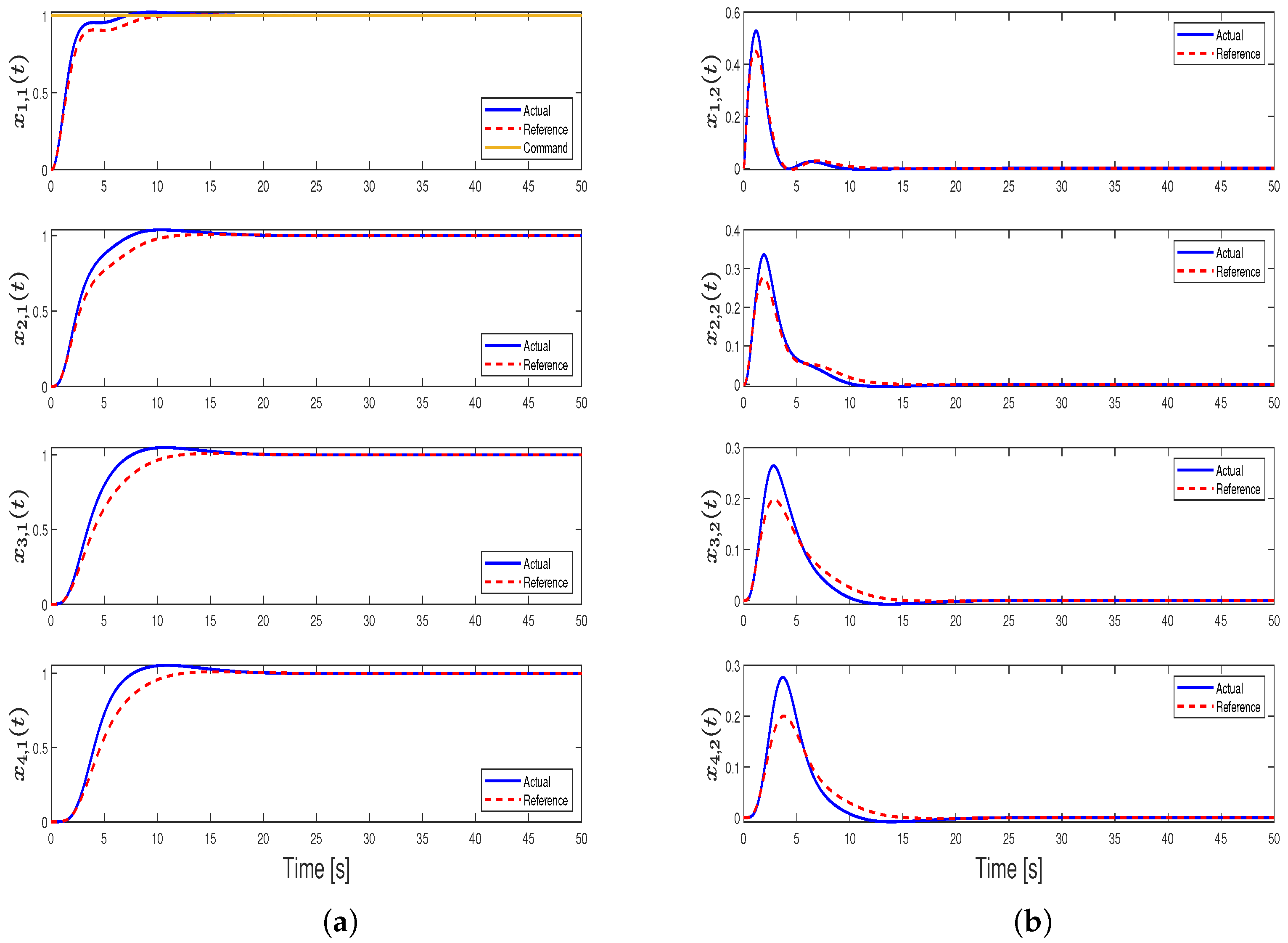
4.2. Case 2—Position and Velocity Consensus

In this case, we investigate the results of applying the controller given in (7) by using position consensus without the damping term (i.e., $k_{d_i}=0$). Hence, the hedging-based reference model dynamics and distributed control algorithm with the same update laws given in (8) and (9) for the $i^{th}$ agent become

$$\begin{array}{ccc}\hfill {\dot{x}}_{{\mathrm{r}}_{i,1}}\left(t\right)& =& x_{{\mathrm{r}}_{i,2}}\left(t\right),\hfill \\ \hfill {\dot{x}}_{{\mathrm{r}}_{i,2}}\left(t\right)& =& -\sum _{i\sim j}\left(x_{{\mathrm{r}}_{i,1}}\left(t\right)-x_{{\mathrm{r}}_{j,1}}\left(t\right)\right)-k_i\left(x_{{\mathrm{r}}_{i,1}}\left(t\right)-c\left(t\right)\right)-\sum _{i\sim j}\left(x_{{\mathrm{r}}_{i,2}}\left(t\right)-x_{{\mathrm{r}}_{j,2}}\left(t\right)\right)\hfill \\ & & +v_i\left(t\right)-u_i\left(t\right),\hfill \end{array}$$

$$\begin{array}{ccc}\hfill u_i\left(t\right)& =& -\sum _{i\sim j}\left(x_{i,1}\left(t\right)-x_{j,1}\left(t\right)\right)-k_i\left(x_{i,1}\left(t\right)-c\left(t\right)\right)-\sum _{i\sim j}\left(x_{i,2}\left(t\right)-x_{j,2}\left(t\right)\right)\hfill \\ & & -{\widehat{\delta }}_i\left(t\right)v_i\left(t\right)-{\widehat{\omega }}_i\left(t\right)x_{i,2}\left(t\right).\hfill \end{array}$$

Here, the above reference model dynamics and controller given in this case yields changes in the analysis of the quadratic stability of $\mathcal{A}\left(\widehat{\mathsf{\Delta }}\left(t\right),\widehat{W}\left(t\right),M\right)$ given in (23) through the resulting controller gain matrix that is set as $K_1=[\mathcal{F}\left(\mathcal{G}\right),\mathcal{L}\left(\mathcal{G}\right)]$. The blue curve represents the feasible actuator bandwidth limits. From Figure 6, Figure 7 and Figure 8, we see that, unlike the first case, agent states’ converge to the desired values and estimated variables converge to constant values. However, there exists oscillation in the command tracking, and it yields degraded transient performances. A feasible actuator bandwidth set for this case can be seen in Figure 9.

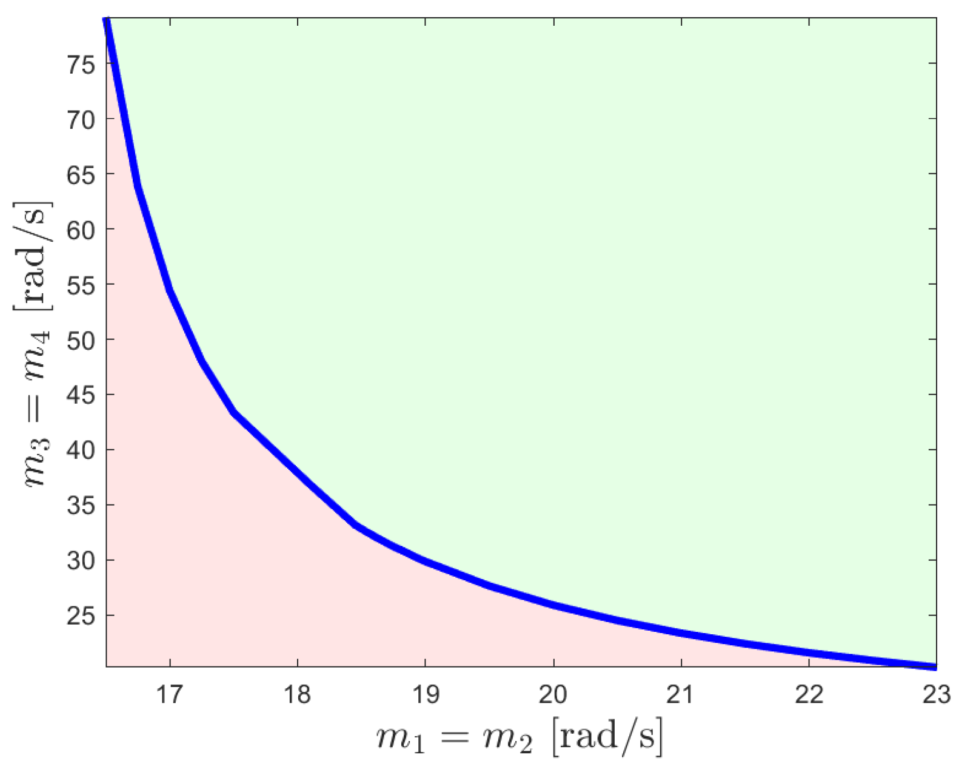
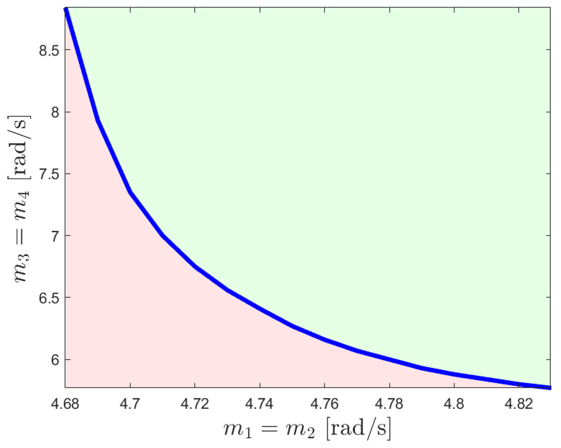
4.3. Case 3—Position Consensus and Damping

In this case, we investigate the results for applying the controller given in (7) by using position consensus and damping without the velocity consensus. The hedging-based reference model dynamics and distributed control algorithm with the same update laws given in (8) and (9) for the $i^{th}$ agent are written as

$$\begin{array}{ccc}& & {\dot{x}}_{{\mathrm{r}}_{i,1}}\left(t\right)=x_{{\mathrm{r}}_{i,2}}\left(t\right),\hfill \\ & & {\dot{x}}_{{\mathrm{r}}_{i,2}}\left(t\right)=-\sum _{i\sim j}\left(x_{{\mathrm{r}}_{i,1}}\left(t\right)-x_{{\mathrm{r}}_{j,1}}\left(t\right)\right)-k_i\left(x_{{\mathrm{r}}_{i,1}}\left(t\right)-c\left(t\right)\right)-k_d{x}_{{\mathrm{r}}_{i,2}}\left(t\right)+v_i\left(t\right)-u_i\left(t\right),\hfill \\ & & u_i\left(t\right)=-\sum _{i\sim j}\left(x_{i,1}\left(t\right)-x_{j,1}\left(t\right)\right)-k_i\left(x_{i,1}\left(t\right)-c\left(t\right)\right)-k_d{x}_{i,2}\left(t\right)-{\widehat{\delta }}_i\left(t\right)v_i\left(t\right)-{\widehat{\omega }}_i\left(t\right)x_{i,2}\left(t\right).\hfill \end{array}$$

Similar to the previous two cases, the reference model dynamics and controller given in this case yields changes in the analysis of the quadratic stability of $\mathcal{A}\left(\widehat{\mathsf{\Delta }}\left(t\right),\widehat{W}\left(t\right),M\right)$ given in (23) through the controller gain matrix that is set as $K_1=[\mathcal{F}\left(\mathcal{G}\right),K_d]$. Here, the blue curve, which represents the feasible actuator set limits, shows the feasible bandwidth set requires higher bandwidth values when compared to Case 2. From Figure 10a,b and Figure 11, we see that, unlike the first and second cases, the agent states converge to the desired values in an asymptotic convergence fashion with minimal oscillations and minimized overshoot. Moreover, estimated unknown control effectiveness and uncertainty reach a constant value faster (see Figure 12a,b) when compared to the previous two cases. The transient response of the closed-loop multi-agent system can also be manipulated by adjusting the damping gain. There is a trade-off between using the velocity consensus term or using the damping term in addition to the position consensus term. Using velocity consensus allows for operation with slower actuators, but yields oscillatory transient behavior with overshoot, while using the damping term instead requires faster actuators, but the transient response is smoother. A promising solution to overcome this trade-off is using the full controller given in (7), which is investigated in the next case. The feasible actuator bandwidth set for this case can be seen in Figure 13.

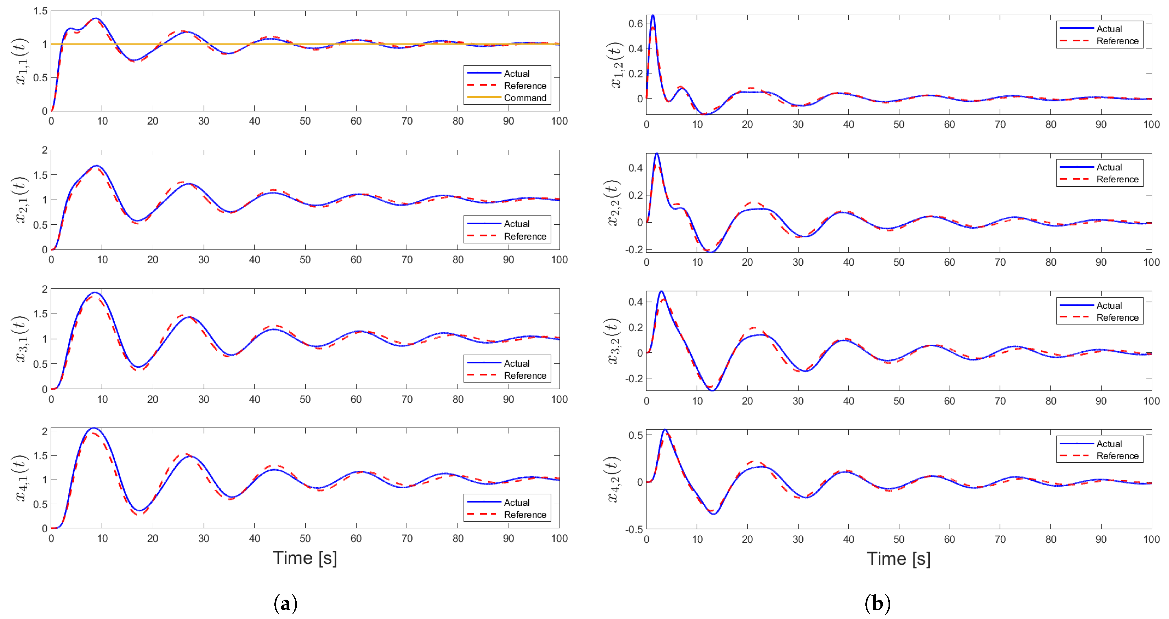
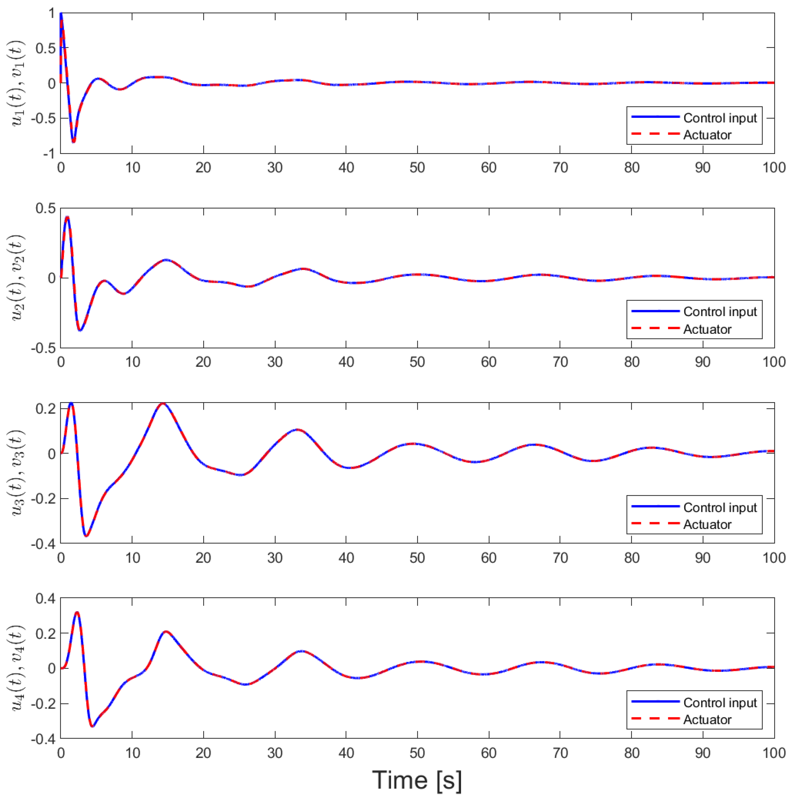
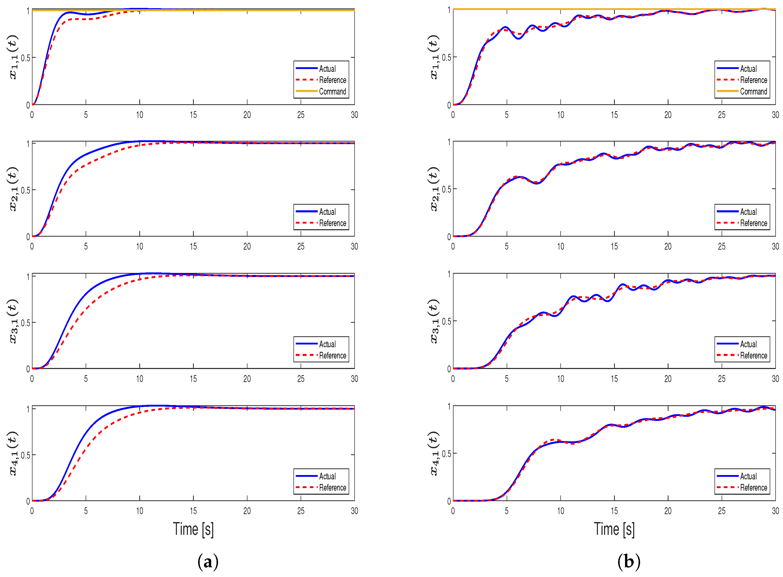
4.4. Case 4—Position, Velocity Consensus, and Damping (Main Result)

In this case, we utilize the hedging-based reference model given in (5) and (6) and the distributed control algorithm provided in (7) with the same update laws given in (8) and (9). By using these dynamics and controller yields $\mathcal{A}\left(\widehat{\mathsf{\Delta }}\left(t\right),\widehat{W}\left(t\right),M\right)$ given in (23) through the controller gain matrix that is as given in (14), $K_1=[\mathcal{F}\left(\mathcal{G}\right),\mathcal{L}\left(\mathcal{G}\right)+K_d]$. The blue curve, which represents the feasible actuator set limits, shows the bandwidth values are less than those in any other case. This provides a great advantage since it enables the use of actuators with much lower bandwidths or, in other words, actuators with higher time constants. From Figure 14, Figure 15 and Figure 16, we see that the transient response is as desired and can be modified by using different damping gains. Since this controller provides a satisfactory transient response and the largest set of feasible actuators, it is superior to the other cases. The feasible actuator bandwidth set for this case can be seen in Figure 17.

In the light of different case results, we can compare the overall numerical results of applying distinct distributed control algorithms to the multi-agent system with system anomalies. As a result, one can first recognize that trying to control a second-order system by using only position consensus without velocity consensus and damping can yield unstable results. However, adding velocity consensus yields asymptotic convergence but does not cancel out the oscillation, which is not a desired transient response for most systems. The solution for this issue is adding a damping term that allows us to obtain a smoother transient response with less or no overshoot, depending on the magnitude of the damping gain. However, increasing the damping gain beyond the optimal value can result in a sluggish system response. Furthermore, adding only damping and not velocity consensus still yields non-oscillatory behavior, and the feasible actuator bandwidth limit increases as seen in Figure 9 and Figure 13. Using all of these terms (position consensus, velocity consensus, and damping) together yields satisfactory transient results that offer asymptotic convergence with minimal oscillation and also the largest feasible actuation bandwidth set.

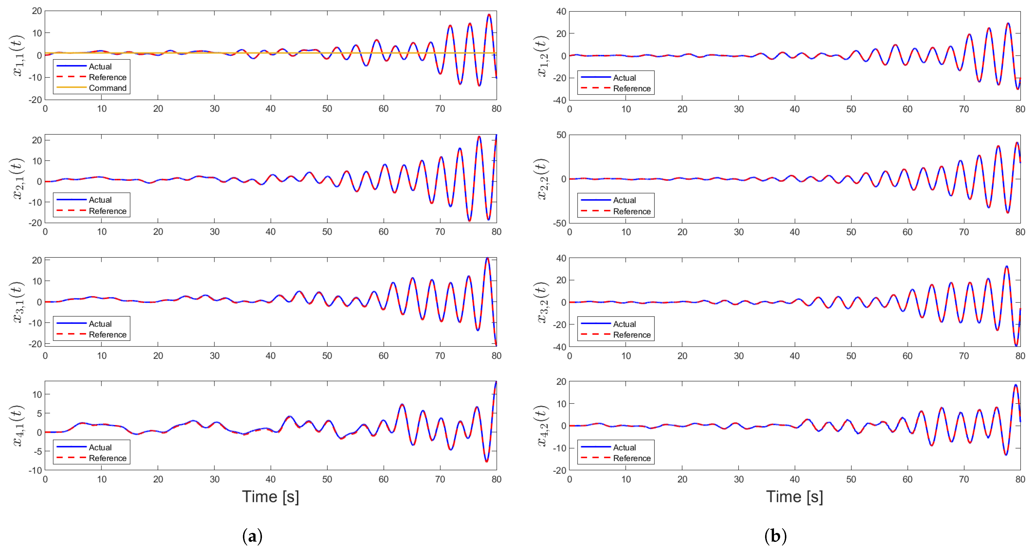
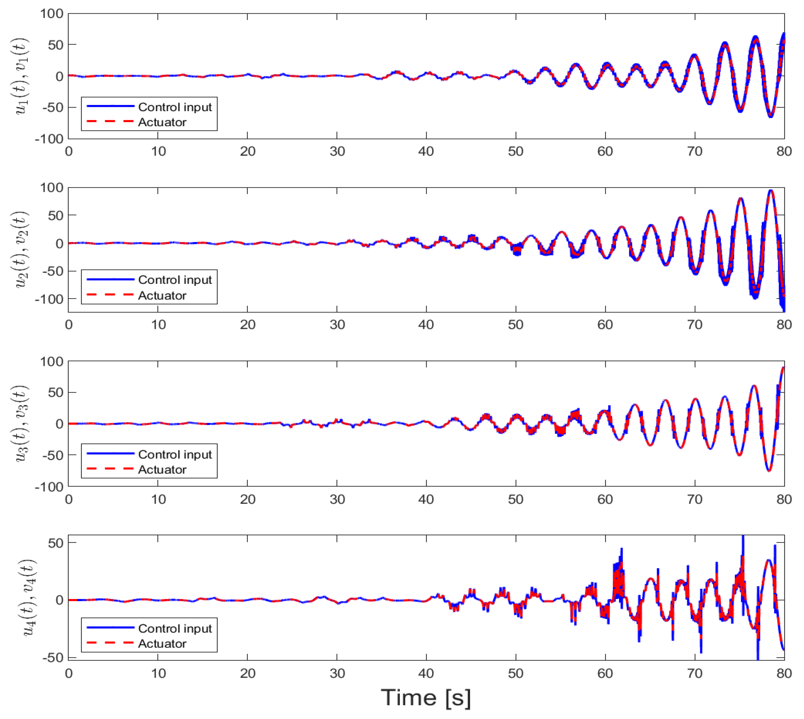
4.5. Case 5—Comparison with the Results in [31]

As a final case, we compare the performance of the proposed distributed adaptive controller with the most recent controller developed in [31] in the context of a multi-agent system with system anomalies. Actuator bandwidth and uncertainty values are selected identically (i.e., $m_1=m_2=20$ rad/s, $m_3=m_4=50$ rad/s, ${\omega }_1={\omega }_3=0.5$, and ${\omega }_2={\omega }_4=0.25$), and, since [31] does not consider unknown control effectiveness, for better comparison, it is assumed that control effectiveness is fully known (i.e., ${\delta }_{1,2,3,4}=0$) for both simulations. Specifically, in [31], the designed control algorithm requires using the integral state to update the control input. As mentioned in Section 1, this yields a poor transient response, delay, and non-robust behavior.

For the simulation of [31], the reference model matrices are selected to be $A_r=[0,1;-0.5,-1]$ and $B_r={[0,0.5]}^{\mathrm{T}}$, which results in the same $K_1$ and $K_2$ values as selected in Case 4. The adaptive learning rates for update laws are selected to be the same as for the results of this paper, which are ${\gamma }_{1i}={\gamma }_{2i}=10$. Also, the damping gain for all agents chosen as $k_{d_{1,2,3,4}}=0.5$, which are, again, the same damping gains selected for the results of this paper. The initial conditions on the system/actuator states and uncertainty estimations are set to zero. Figure 18, Figure 19 and Figure 20 show the resulting simulation comparison.

It is clear that both algorithms converge to the given command. However, the distributed adaptive controller proposed in this paper outperforms the other controller. The main reason behind this is the structure of the control algorithm, where we directly use consensus errors without any integration. In [31], the researchers utilize an integrator-based control law that consists of position and velocity consensus. This integrator structure yields a virtual phase lag between the actual consensus errors and the control input driving the system. This integrator results in oscillation in the transient response. It is possible to see this effect clearly in Figure 19 as the first peak commands are produced within four seconds in our controller while it takes around six seconds for the other controller.

5. Conclusions

In this paper, to obtain a fast update/response and improved transient performance, we designed a novel distributed adaptive control law. We showed that one can drive a set of agents with double-integrator dynamics in a leader–follower fashion in the presence of uncertainty, unknown control effectiveness, and actuator dynamics. For the results of this paper, we introduced a novel hedging-based reference model with second-order dynamics. We showed that the proposed distributed adaptive controller tracks a novel hedging-based reference model asymptotically. Specifically, we showed the stability of the overall closed-loop multi-agent system by utilizing Lyapunov Stability Theory. We also analyzed an additional stability condition that is a result of using the hedging-based reference model by using a Linear Matrix Inequalities method to show the boundedness of the reference model and actuator states. Finally, we illustrated the efficacy of the distributed adaptive controller and performance results with a simulation based on an undirected and connected line graph in five cases. One can consider applying the theoretical solution to an experimental background as a future research direction.

References

1. Lewis, F.L.; Zhang, H.; Hengster-Movric, K.; Das, A. Cooperative Control of Multi-Agent Systems: Optimal and Adaptive Design Approaches; Springer Science & Business Media: London, UK, 2013. [Google Scholar]
2. Olfati-Saber, R.; Fax, J.A.; Murray, R.M. Consensus and cooperation in networked multi-agent systems. Proc. IEEE 2007, 95, 215–233. [Google Scholar] [CrossRef]
3. Shamma, J. Cooperative Control of Distributed Multi-Agent Systems; John Wiley & Sons: Hoboken, NJ, USA, 2008. [Google Scholar]
4. Bullo, F.; Cortéz, J.; Martinéz, S. Distributed Control of Robotic Networks; Princeton University Press: Princeton, NJ, USA, 2009. [Google Scholar]
5. Mesbahi, M.; Egerstedt, M. Graph Theoretic Methods in Multiagent Networks; Princeton University Press: Princeton, NJ, USA, 2010. [Google Scholar]
6. Cao, Y.; Yu, W.; Ren, W.; Chen, G. An overview of recent progress in the study of distributed multi-agent coordination. IEEE Trans. Ind. Inform. 2012, 9, 427–438. [Google Scholar] [CrossRef]
7. Rossi, F.; Bandyopadhyay, S.; Wolf, M.T.; Pavone, M. Multi-Agent Algorithms for Collective Behavior: A structural and application-focused atlas. arXiv 2021, arXiv:2103.11067. [Google Scholar]
8. Saber, R.O.; Murray, R.M. Consensus protocols for networks of dynamic agents. In Proceedings of the 2003 American Control Conference, Denver, CO, USA, 4–6 June 2003; pp. 951–956. [Google Scholar]
9. Blondel, V.D.; Hendrickx, J.M.; Olshevsky, A.; Tsitsiklis, J.N. Convergence in multiagent coordination, consensus, and flocking. In Proceedings of the 44th IEEE Conference on Decision and Control, Seville, Spain, 15 December 2005; pp. 2996–3000. [Google Scholar]
10. Hong, Y.; Hu, J.; Gao, L. Tracking control for multi-agent consensus with an active leader and variable topology. Automatica 2006, 42, 1177–1182. [Google Scholar] [CrossRef]
11. Ren, W.; Sorensen, N. Distributed coordination architecture for multi-robot formation control. Robot. Auton. Syst. 2008, 56, 324–333. [Google Scholar] [CrossRef]
12. Ren, W.; Atkins, E. Distributed multi-vehicle coordinated control via local information exchange. Int. J. Robust Nonlinear Control IFAC-Affil. J. 2007, 17, 1002–1033. [Google Scholar] [CrossRef]
13. Ren, W. Consensus strategies for cooperative control of vehicle formations. IET Control Theory Appl. 2007, 1, 505–512. [Google Scholar] [CrossRef]
14. Ren, W. On Consensus Algorithms for Double-Integrator Dynamics. IEEE Trans. Autom. Control 2008, 53, 1503–1509. [Google Scholar] [CrossRef]
15. Abdessameud, A.; Tayebi, A. On consensus algorithms for double-integrator dynamics without velocity measurements and with input constraints. Syst. Control Lett. 2010, 59, 812–821. [Google Scholar] [CrossRef]
16. Egerstedt, M.; Hu, X. Formation constrained multi-agent control. IEEE Trans. Robot. Autom. 2001, 17, 947–951. [Google Scholar] [CrossRef]
17. Jadbabaie, A.; Lin, J.; Morse, A.S. Coordination of groups of mobile autonomous agents using nearest neighbor rules. IEEE Trans. Autom. Control 2003, 48, 988–1001. [Google Scholar] [CrossRef]
18. Dimarogonas, D.V.; Egerstedt, M.; Kyriakopoulos, K.J. A leader-based containment control strategy for multiple unicycles. In Proceedings of the 45th IEEE Conference on Decision and Control, San Diego, CA, USA, 13–15 December 2006; pp. 5968–5973. [Google Scholar]
19. Dimarogonas, D.V.; Kyriakopoulos, K.J. A connection between formation control and flocking behavior in nonholonomic multiagent systems. In Proceedings of the 2006 IEEE International Conference on Robotics and Automation, ICRA 2006, Orlando, FL, USA, 15–19 May 2006; pp. 940–945. [Google Scholar]
20. Talebi, S.P.; Werner, S.; Huang, Y.F.; Gupta, V. Distributed Algebraic Riccati Equations in Multi-Agent Systems. In Proceedings of the 2022 European Control Conference (ECC), London, UK, 12–15 July 2022; pp. 1810–1817. [Google Scholar]
21. Fattahi, S.; Fazelnia, G.; Lavaei, J.; Arcak, M. Transformation of optimal centralized controllers into near-globally optimal static distributed controllers. IEEE Trans. Autom. Control 2018, 64, 66–80. [Google Scholar] [CrossRef]
22. Das, A.; Lewis, F.L. Distributed adaptive control for synchronization of unknown nonlinear networked systems. Automatica 2010, 46, 2014–2021. [Google Scholar] [CrossRef]
23. Yucelen, T.; Johnson, E.N. Control of multivehicle systems in the presence of uncertain dynamics. Int. J. Control 2013, 86, 1540–1553. [Google Scholar] [CrossRef]
24. Wang, W.; Wen, C.; Huang, J. Distributed adaptive asymptotically consensus tracking control of nonlinear multi-agent systems with unknown parameters and uncertain disturbances. Automatica 2017, 77, 133–142. [Google Scholar] [CrossRef]
25. Sarsilmaz, S.B.; Yucelen, T. A Distributed Adaptive Control Approach for Heterogeneous Uncertain Multiagent Systems. In Proceedings of the 2018 AIAA Guidance, Navigation, and Control Conference, Kissimmee, FL, USA, 8–12 January 2018. [Google Scholar]
26. Dogan, K.M.; Gruenwald, B.C.; Yucelen, T.; Muse, J.A.; Butcher, E.A. Distributed adaptive control of networked multiagent systems with heterogeneous actuator dynamics. In Proceedings of the 2017 American Control Conference (ACC), Seattle, WA, USA, 24–26 May 2017. [Google Scholar]
27. Kurttisi, A.; Aly, I.A.; Dogan, K.M. Coordination of Uncertain Multiagent Systems with Non-Identical Actuation Capacities. In Proceedings of the 2022 IEEE 61st Conference on Decision and Control (CDC), Cancun, Mexico, 6–9 December 2022; pp. 3947–3952. [Google Scholar]
28. Sarioglu, E.; Kurttisi, A.; Dogan, K.M. Experimental Results on Composing Cooperative Behaviors in Networked Mobile Robots in the Presence of Unknown Control Effectiveness. In Proceedings of the AIAA SCITECH 2023 Forum, National Harbor, MD, USA, 23–27 January 2023; pp. 5–8. [Google Scholar]
29. Mirzaei, M.J.; Ghaemi, S.; Badamchizadeh, M.A.; Baradarannia, M. Adaptive super-twisting control for leader-following consensus of second-order multi-agent systems based on time-varying gains. ISA Trans. 2023, 140, 144–156. [Google Scholar] [CrossRef]
30. Dogan, K.M.; Yucelen, T.; Muse, J.A. Stability Verification for Uncertain Multiagent Systems in the Presence of Heterogeneous Coupled and Actuator Dynamics. In Proceedings of the AIAA Scitech 2021 Forum, Virtual Event, 11–15 & 19–21 January 2021. [Google Scholar]
31. Dogan, K.M.; Gruenwald, B.C.; Yucelen, T.; Muse, J.A.; Butcher, E.A. Distributed adaptive control and stability verification for linear multiagent systems with heterogeneous actuator dynamics and system uncertainties. Int. J. Control 2019, 92, 2620–2638. [Google Scholar] [CrossRef]
32. Godsil, C.; Royle, G. Algebraic Graph Theory; Springer: New York, NY, USA, 2001. [Google Scholar]
33. Khalil, H.K. Adaptive output feedback control of nonlinear systems represented by input-output models. IEEE Trans. Autom. Control 1996, 41, 177–188. [Google Scholar] [CrossRef]
34. Lavretsky, E.; Wise, K.A. Robust Adaptive Control. In Robust and Adaptive Control; Springer: London, UK, 2013; pp. 317–353. [Google Scholar]
35. Boyd, S.; El Ghaoui, L.; Feron, E.; Balakrishnan, V. Linear Matrix Inequalities in System and Control Theory; SIAM: Philadelphia, PA, USA, 1994. [Google Scholar]
36. Khalil, H.K. Nonlinear Systems; Prentice Hall: Upper Saddle River, NJ, USA, 2002. [Google Scholar]
37. Löfberg, J. YALMIP: A Toolbox for Modeling and Optimization in MATLAB. In Proceedings of the 2004 IEEE International Conference on Robotics and Automation (IEEE Cat. No. 04CH37508), New Orleans, LA, USA, 26 April–1 May 2004. [Google Scholar]
38. Mosek ApS. The MOSEK Optimization Toolbox for MATLAB Manual; Version 9.3; Mosek ApS: Copenhagen, Denmark, 2022. [Google Scholar]
Figure 1. Illustration of the structure of the closed-loop system.
Electronics 13 01142 g001
Figure 3. State trajectories x i ( t ) for Case 1: (a) position trajectories for each agent and (b) velocity trajectories for each agent.
Electronics 13 01142 g003
Figure 4. Distributed adaptive control inputs u i ( t ) and actuator outputs v i ( t ) for Case 1.
Electronics 13 01142 g004
Figure 5. Adaptive estimates δ ^ i ( t ) and ω ^ i ( t ) for Case 1: (a) adaptive control effectiveness estimates δ ^ i ( t ) and (b) adaptive uncertainty estimates ω ^ i ( t ) .
Electronics 13 01142 g005
Figure 6. State trajectories x i ( t ) for Case 2: (a) position trajectories for each agent and (b) velocity trajectories for each agent.
Electronics 13 01142 g006
Figure 7. Distributed adaptive control inputs u i ( t ) and actuator outputs v i ( t ) for Case 2.
Electronics 13 01142 g007
Figure 8. Adaptive estimates δ ^ i ( t ) and ω ^ i ( t ) for Case 2: (a) adaptive control effectiveness estimates δ ^ i ( t ) and (b) adaptive uncertainty estimates ω ^ i ( t ) .
Electronics 13 01142 g008
Figure 9. Actuator bandwidth set that makes A Δ ^ ( t ) , W ^ ( t ) , M quadratically stable after LMI analysis for Case 2. The blue curve represents the bandwidth limits, where the area highlighted with green refers to the feasible set of actuator bandwidths that provide quadratic stability and red refers to the unfeasible set.
Electronics 13 01142 g009
Figure 10. State trajectories x i ( t ) for Case 3: (a) position trajectories for each agent and (b) velocity trajectories for each agent.
Electronics 13 01142 g010
Figure 11. Distributed adaptive control inputs u i ( t ) and actuator outputs v i ( t ) for Case 3.
Electronics 13 01142 g011
Figure 12. Adaptive estimates δ ^ i ( t ) and ω ^ i ( t ) for Case 3: (a) adaptive control effectiveness estimates δ ^ i ( t ) and (b) adaptive uncertainty estimates ω ^ i ( t ) .
Electronics 13 01142 g012
Figure 13. Actuator bandwidth set that makes A Δ ^ ( t ) , W ^ ( t ) , M quadratically stable after LMI analysis for Case 3. The blue curve represents the bandwidth limits, where the area highlighted with green refers to the feasible set of actuator bandwidths that provide quadratic stability, and red refers to the unfeasible set.
Electronics 13 01142 g013
Figure 14. State trajectories x i ( t ) for Case 4: (a) position trajectories for each agent and (b) velocity trajectories for each agent.
Electronics 13 01142 g014
Figure 15. Distributed adaptive control inputs u i ( t ) and actuator outputs v i ( t ) for Case 4.
Electronics 13 01142 g015
Figure 16. Adaptive estimates δ ^ i ( t ) and ω ^ i ( t ) for Case 4: (a) adaptive control effectiveness estimates δ ^ i ( t ) and (b) adaptive uncertainty estimates ω ^ i ( t ) .
Electronics 13 01142 g016
Figure 17. Actuator bandwidth set that makes A Δ ^ ( t ) , W ^ ( t ) , M quadratically stable after LMI analysis for Case 4. The blue curve represents the bandwidth limits, where the area highlighted with green refers to the feasible set of actuator bandwidths that provide quadratic stability, and red refers to the unfeasible set.
Electronics 13 01142 g017
Figure 18. Position trajectories comparison for Case 5: (a) position trajectories for our controller and (b) position trajectories for controller in [31].
Electronics 13 01142 g018
Figure 19. Velocity trajectories comparison for Case 5: (a) velocity trajectories for our controller and (b) velocity trajectories for controller in [31].
Electronics 13 01142 g019
Figure 20. Distributed adaptive control inputs u i ( t ) and actuator outputs v i ( t ) comparison for Case 5: (a) distributed adaptive control inputs u i ( t ) and actuator outputs v i ( t ) and (b) distributed adaptive control inputs u i ( t ) and actuator outputs v i ( t ) in [31].
Electronics 13 01142 g020