An Aero-Engine Classification Method Based on Fourier Transform Infrared Spectrometer Spectral Feature Vectors

Abstract

Aiming at the classification identification problem of aero-engines, this paper adopts a telemetry Fourier transform infrared spectrometer to collect aero-engine hot jet infrared spectrum data and proposes an aero-engine classification identification method based on spectral feature vectors. First, aero-engine hot jet infrared spectrum data are acquired and measured; meanwhile, the spectral feature vectors based on CO₂ are constructed. Subsequently, the feature vectors are combined with the seven mainstream classification algorithms to complete the training and prediction of the classification model. In the experiment, two Fourier transform infrared spectrometers, EM27 developed by Bruker and a self-developed telemetry FT-IR spectrometer, were used to telemeter the hot jet of three aero-engines to obtain infrared spectral data. The training data set and test data set were randomly divided in a ratio of 3:1. The model training of the training data set and the label prediction of the test data set were carried out by combining spectral feature vectors and classification algorithms. The classification evaluation indicators were accuracy, precision, recall, confusion matrix, and F1-score. The classification recognition accuracy of the algorithm was 98%. This paper has considerable significance for the fault diagnosis of aero-engines and classification recognition of aircrafts.

1. Introduction

Infrared spectroscopy technology [1,2,3] is a technique for detecting the molecular structure and chemical composition of substances. This technology utilizes the energy level transition of molecules in substances under infrared radiation to measure the wavelength and intensity of absorbed or emitted light, producing specific spectrogram, which are used to analyze and judge the chemical bonds and structures of substances. This technology has significant research applications in environmental monitoring [4], garbage classification [5], and life chemistry [6]. The Fourier transform infrared spectrometer (FT-IR spectrometer) [7,8,9] is an important means of measuring infrared spectra. It obtains interferogram through an interferometer and restores the interferogram to spectrogram based on Fourier transform. Passive FT-IR is frequently used for the detection of atmospheric pollutants. It has the ability to collect data from any direction, allowing for all-weather, continuous, long-distance, real-time monitoring and rapid analysis of targets.

The classification characteristics of aero-engines are frequently related to fuel type, combustion method, and emission characteristics. Different types of aero-engines produce different gas components and emissions during the combustion process. The vibration and rotation of these molecules form specific infrared absorption and emission spectra. By analyzing the infrared spectra of aero-engine hot jet, the characteristics of the gas components and emissions produced by aero-engine combustion can be obtained. After a considerable number of hot jet infrared spectra are analyzed, a spectral feature library will be established, then the types of aero-engines are going to be determined so that the identification of aero-engines will be realized.

In this paper, an algorithm for the classification and recognition of aero-engines is proposed, which combines the infrared spectrum feature vectors of aero-engine hot jet with the current mainstream classifiers. The classifiers include supervised learning method SVM, integrated learning methods XGBoost, CatBoost, AdaBoost, Random Forest, LightGBM, and a neural network method. Accuracy, precision, recall, F1 value, and confusion matrix are used as classification evaluation criteria. After many experiments, the accuracy of the classification of aero-engines has reached 98%.

The major contributions of this paper are as follows:

• The infrared spectrum detection method for aero-engine hot jet is used as the basis and data source input of the identification of aero-engines. Aero-engine hot jet is an important infrared radiation characteristic of aero-engine, and the infrared spectrum provides the characteristic information of substances at the molecular level, so it is more scientific to utilize this method for classification.
• FT-IR is used to measure the infrared spectrum information of aero-engine hot jet. An FT-IR spectrometer has the advantages of fast scanning speed, excellent resolution, wide measurement spectral range, and high measurement accuracy. It can achieve exceptional spectral measurement, which is of great significance for the non-contact classification and recognition of aero-engines.

The architecture of this paper is as follows: Section 1 describes the infrared spectroscopy technology, and this paper uses the classification method, innovation, and article architecture; in Section 2, the spectral components of the hot jet are analyzed, and the construction method of spectral feature vectors is proposed; Section 3 introduces seven mainstream classifier methods; Section 4 describes the experimental content, including the experimental design of aero-engine spectrum acquisition, data set production, spectral feature vectors extraction, and the accuracy evaluation of classification prediction results; Section 5 summarizes the paper and puts forward the idea of the next research direction.

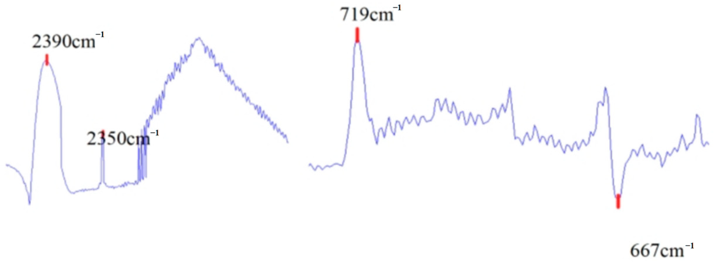
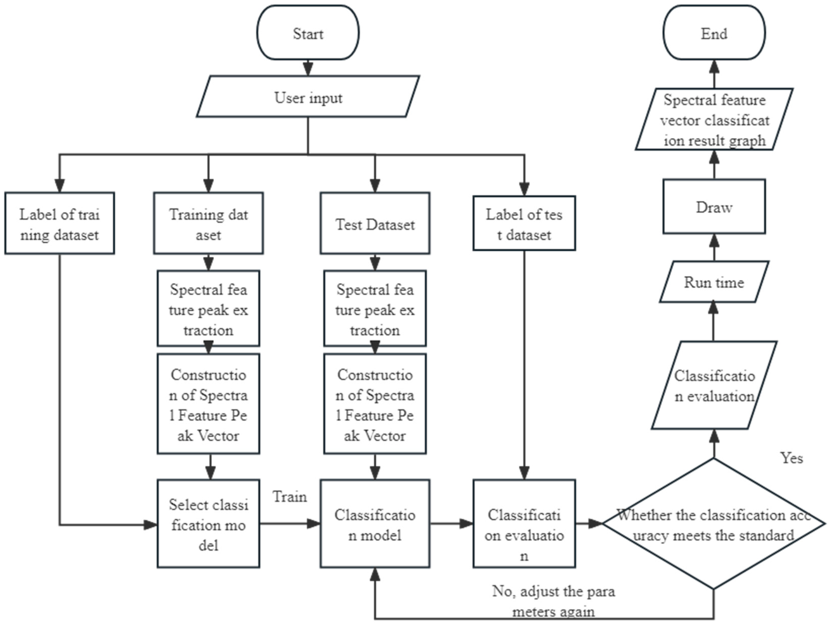
2. Spectral Feature Analysis and Spectral Feature Vector Construction

In this section, the brilliant temperature spectrum (BTS) and components of aero-engine hot jet are analyzed, and a method of constructing spectral feature vectors based on CO₂ characteristic peaks is proposed.

When passive FT-IR is used in gas detection and identification studies, the method of calculating the BTS with a constant baseline can be utilized due to the high emissivity of most of the substances in nature that serve as the background. The brilliant temperature [10,11] of a material object is equivalent to the temperature of a blackbody at the same wavelength when the intensity of the spectral radiation of the material object and the blackbody are equal. It is based on equal brightness and is utilized to characterize the material object’s own radiation. The use of BTS does not require pre-measurement of the background spectrum and enables the target gas characteristics to be extracted directly from the BTS analysis.

In order to obtain the BTS from the passive infrared spectrum, it is necessary to first deduct the spectral signal measured by the spectrometer from the bias and response of the instrument to obtain the spectral radiance spectrum entering the spectrometer, and from the radiance spectrum obtained, the equivalent temperature of the radiance spectrum $T\left(v\right)$ can be calculated according to Planck’s law of radiation by transforming Planck’s formula to obtain the following formula:

$$T(v)=\frac{hcv}{k\ln \left\{\right[L\left(v\right)+2h{c}^2{v}^3]/L(v\left)\right\}}$$

(1)

where $h$ is Planck’s constant with a value of 6.62607015 × 10^−34 J·S, $c$ represents the speed of light with a value of 2.998 × 10^8 m/s, $v$ is the wave number in cm⁻¹, $k$ is Boltzmann’s constant with a value of 1.380649 × 10^−23 J/K, and $L\left(v\right)$ represents the radiance about the wave number.

The experimentally measured infrared spectra of aero-engine hot jets of three turbojet engines are presented in Figure 1, where the horizontal coordinates are the wave numbers and the vertical coordinates are the BTS.

The emission products of an aero-engine typically include oxygen (O₂), nitrogen (N₂), carbon dioxide (CO₂), steam (H₂O), carbon monoxide (CO), et al. The combustion products are primarily divided into ① air composition not participating in combustion, including O₂ and N₂, ② products of combustion reactions, mainly NO_x, ③ the end product of an ideal combustion process, including CO₂, H₂O, and CO [12].

Based on the main emissions of the aero-engines and the measured infrared spectral data of the aero-engines, the peaks of the three most likely products of combustion, CO₂, H₂O, and CO, were compared and analyzed. It was discovered that in the spectral curve, the characteristic peaks of CO₂ at 667 cm⁻¹ and 2349 cm⁻¹ were obvious and stable, the spectrum of CO at the characteristic band of 2000–2222 cm⁻¹ gradually weakened with the increase of rotational speed, and the characteristic peaks of H₂O were not obvious and not informative. Therefore, the two characteristic peaks (667 cm⁻¹ and 2350 cm⁻¹) of CO₂ in the mid-wave infrared (MWIR) region (400–4000 cm⁻¹) and the two stable and obvious characteristic peaks (719 cm⁻¹ and 2390 cm⁻¹) in the measured spectral curve were selected for the construction of spectral feature vectors. In this paper, the spectral feature vectors are constructed based on the BTS, and the numerical difference of the BTS is related to the exhaust temperature of the aero-engines as well as the concentration and temperature of the gas in the hot jet.

Four characteristic peaks in the MWIR region of the BTS of the measured aero-engine hot jet were selected for the construction of spectral feature vectors, and the corresponding wave numbers of the peaks are 2350 cm⁻¹, 2390 cm⁻¹, 719 cm⁻¹, and 667 cm⁻¹; their locations are shown in Figure 2 below:

Spectral feature vectors $a=[a_1,a_2]$ are composed of individual spectra by calculating the peak difference between 2390 cm⁻¹ and 2350 cm⁻¹ and the peak difference between 719 cm⁻¹ and 667 cm⁻¹.

$$\begin{array}{c}{a}_1=T_{v=2390{\mathrm{c}\mathrm{m}}^{-1}}-T_{v=2350{\mathrm{c}\mathrm{m}}^{-1}}\\ a_2=T_{v=719{\mathrm{c}\mathrm{m}}^{-1}}-T_{v=677{\mathrm{c}\mathrm{m}}^{-1}}\end{array}$$

(2)

Affected by the environment, the peak positions of the selected characteristic peaks may be shifted, the four characteristic peaks of 2350 cm⁻¹, 2390 cm⁻¹, 719 cm⁻¹, and 667 cm⁻¹ of the experimentally measured infrared spectral data are extracted from the area range where the maximum and minimum peaks are located for the extraction of spectral feature vectors, and the specific selection of the threshold range is shown in

Table 1. Characteristic peak threshold takes the value range.

Characteristic Peak Type	Emission Peak (cm−1)			Absorption Peak (cm−1)
Peak standard features	2350	2390	719	667
Characteristic peak range values	2350.5–2348	2377–2392	722–718	666.7–670.5

:

3. Spectral Eigenvector Classification Methods

This section provides a brief description of the mainstream classifiers SVM [13,14,15], XGBoost 1.0 [16,17], CatBoost 1.0.4 [18,19,20], AdaBoost [21], Random Forest [22], LightGBM [23], and neural network [24,25] classifiers.

The current mainstream classification methods are supervised learning methods, unsupervised learning methods, semi-supervised learning methods, reinforcement learning methods, deep learning methods, and ensemble learning methods. Supervised learning methods are methods that use training data with labels to construct a model used to classify new samples, including decision tree, support vector machines (SVM), and logistic regression. Ensemble learning methods include Bagging and Boosting, where Bagging is characterized by the absence of strong dependencies between individual evaluators, and a series of individual learners can be generated in parallel, representing the algorithm Random Forest; Boosting is characterized by the presence of strong dependencies between individual learners, and a series of individual learners basically Boosting is characterized by a strong dependency relationship between individual learners, and a series of individual learners basically need to be generated serially, representing algorithms like AdaBoost, XGBoost, LightGBM, etc.

In view of the characteristics of the aero-engine infrared spectral data and the way of measurement in this paper, it is more appropriate to use the training data set, test data set, and label set for model training to carry out classification and prediction. In this paper, SVM, XGBoost, CatBoost, AdaBoost, Random Forest, LightGBM, and neural network algorithms are used in conjunction with spectral feature vectors to complete the classification task of the aero-engines.

①

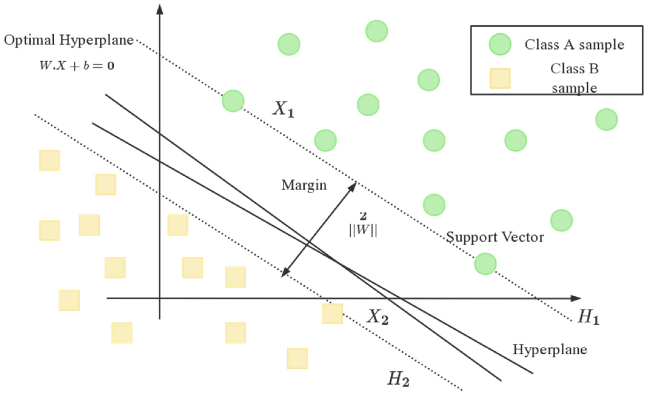
Support vector machine (SVM) classification method

SVM is a kernel function-based classification algorithm machine learning binary classification model for both binary and multi-classification problems. The main task of the SVM model is to find the optimal over-planning for classifying the data points. For binary classification, the SVM algorithm is shown in Figure 3:

SVM classifies the data by hyperplane $y$, which can be expressed as

$$y={\omega }^T\mathrm{x}+b$$

(3)

Calculate the hyperplane equations, the thresholds on both sides, and the optimization function for the best vector in the hyperplane. Define the margin line as passing through the nearest point in each class to obtain the equation for the boundary line as:

$$\begin{array}{c}{\omega }^{T}x+b=0\\ {\omega }^{T}x+b=1\\ {\omega }^{T}x+b=-1\end{array}$$

(4)

where, $\begin{array}{c}{\omega }^{T}x+b=0\end{array}$ is the hyperplane equation, $\begin{array}{c}{\omega }^{T}x+b=1\end{array}$ is the edge line equation for the positive region, and $\begin{array}{c}{\omega }^{T}x+b=-1\end{array}$ is the edge line equation for the region with negative values.

Finding the distance between two edges can be accomplished by the following:

$$\begin{array}{c}{\omega }^T(x_2-x_1)=2\\ x_2-x_1=\frac{2}{\parallel {\omega }^T\parallel }\end{array}$$

(5)

Maximize the margin line function to find the optimal threshold. The final SVM model is obtained:

$$({\omega }^{*},b^{*})máx\frac{2}{\parallel w^T\parallel }{y}_i^{*}({\omega }^T{x}_i+{\mathrm{b}}_i)>=1$$

(6)

The SVM algorithm is suitable for high-dimensional spatial data processing and has good performance in the field of text classification and image recognition, and at the same time, it can maintain good performance when small amounts of sample data are processed. The SVM algorithm is also one of the most commonly used algorithms in current classification tasks.

②

XGBoost classification method

XGBoost is an efficient classification and regression algorithm based on gradient boosted decision trees. The XGBoost algorithm generates multiple decision trees in an iterative manner by integrating weak classifiers and training based on the residuals of the previous decision tree and completely integrates multiple decision trees to improve the performance of the model and complete the classification.

In the XGBoost classifier, firstly, the training data set ${\left\{\right(x_i\cdot y_i\left)\right\}}_{i=1}^N$, the differentiable loss function $L(y,F(x\left)\right)$, multiple weak learning M, and the learning rate α are defined as the input parameters of the XGBoost model.

Initialization operations are performed on the model manipulating constant values:

$${\hat{f}}_{(0)}(x)=\underset{\theta }{\arg min}\sum _{i=1}^{N}L(y_i,\theta )$$

(7)

As the model starts from 1 iteration to M, the gradient is first calculated:

$${\hat{g}}_m(x_i)={\left[\frac{\partial L(y_i,f(x_i))}{\partial f(x_i)}\right]}_{f(x)-{\hat{f}}_{(m-1)}(x)}$$

(8)

Second, calculate the Hessians matrix:

$${\hat{h}}_m(x_i)={\left[\frac{{\partial }^{2}L(y_i,f(x_i))}{\partial f{(x_i)}^2}\right]}_{f(x)-{\hat{f}}_{(m-1)}(x)}$$

(9)

Fit the base learner to the training data set ${\{x_i,-\frac{{\hat{g}}_m(x_i)}{{\hat{h}}_m(x_i)}\}}_{i=1}^N$ evolutionary optimization of the formula is obtained:

$${\hat{\phi }}_m=\underset{\phi \in \mathsf{\Phi }}{\arg min}\sum _{i=1}^N\frac{1}{2}{h}_m(x_i){[\phi (x_i)-\frac{{\hat{g}}_m(x_i)}{\widehat{h_m}(x_i)}]}^2$$

(10)

$${\hat{f}}_m(x)=\alpha {\hat{\varphi }}_m(x)$$

(11)

Finally, the model is updated:

$${\hat{f}}_{(m)}(x)={\hat{f}}_{(m-1)}(x)+{\hat{f}}_m(x)$$

(12)

After the iteration is completed, the output of the final model equation is:

$$\hat{f}(x)={\hat{f}}_{(M)}(x)=\sum _{m=0}^M{\hat{f}}_m(x)$$

(13)

The XGBoost algorithm shows higher performance and efficiency in classification tasks on large-scale data sets. The following are some benefits of the XGBoost algorithm: firstly, it is extraordinarily efficient in handling large-scale data; it supports L1 and L2 regularization, which helps to prevent over-fitting; it is effective to automatically select the salient features, which reduces the work of feature engineering; it supports a variety of loss functions, which can handle multiple tasks, such as regression, classification, sorting, etc.; it is capable of utilizing multiple core processors in parallel, sorting, and many other tasks; it is able to perform parallel computation using multi-core processors.

③

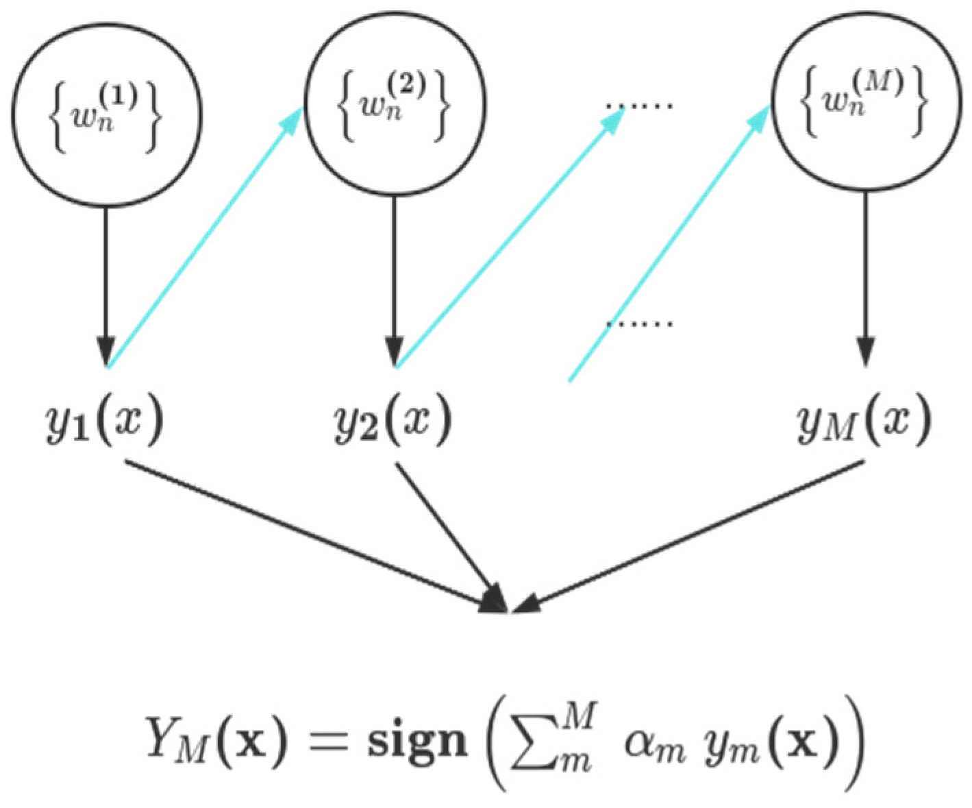
AdaBoost classification method

The AdaBoost algorithm is an adaptive enhancement algorithm for ensemble learning; the method is used to add and train new weak decision makers serially and weigh the combination of decision makers so that the loss function continues to decrease until the addition of decision makers is ineffective and finally all the decision makers are integrated into one whole for decision making. The AdaBoost algorithm is illustrated in Figure 4, and the arrows in the figure indicate the data flow direction:

First, the AdaBoost algorithm defines the training data set as $T=\left\{\right(x_1,y_1),(x_2,y_2),\dots ,(x_n,y_n\left)\right\}$, where $y\in \{-1,+1\}$, the learner is defined as $G_m\left(x\right)$, the training session is set as M, and the initial weight distribution is set as $w_i^{\left(1\right)}=\frac{1}{N}$, where $i=\mathrm{1,2},3,\dots ,N$.

During the training iterations, the base learner $G_m\left(x\right)$ is first obtained by learning using a training data set with a distribution of power values:

$$G_m(x)=\underset{G(x)}{\arg min}\sum _{i=1}^N{w}_i^{(m)}\mathbb{I}(y_i\ne G(x_i))$$

(14)

Based on $G_m\left(x\right)$, calculate the error rate of the learner $G_m\left(x\right)$ on the training data set:

$${ϵ}_m=\frac{\sum _{i=1}^N{w}_i^{\left(m\right)}\mathbb{I}(y_i\ne G_m(x_i\left)\right)}{\sum _{i=1}^N{w}_i^{\left(m\right)}}$$

(15)

Calculate the coefficient ${\alpha }_m$ of $G_m\left(x\right)$:

$${\alpha }_m=\frac{1}{2}\mathrm{l}\mathrm{n}\frac{1-{ϵ}_m}{{ϵ}_m}$$

(16)

Update the sample weight distribution $w_i^{(m+1)}$:

$$w_i^{(m+1)}=\frac{w_i^{\left(m\right)}{e}^{-y_i{\alpha }_m\left({\xi }_m\right(x_i)}}{Z^{\left(m\right)}},i=\mathrm{1,2},3\cdots N$$

(17)

where $Z^{\left(m\right)}$ is the normalization factor, $Z^{\left(m\right)}=\sum _{i=1}^N{w}^{\left(m\right)}i{e}^{-y_i{\alpha }_m{G}_m\left(x_i\right)}$, which ensures that all $w_i^{(m+1)}$ constitute a distribution.

The final output of the model $G\left(x\right)$:

$$G(x)=\mathrm{s}\mathrm{i}\mathrm{g}\mathrm{n}\left[\sum _{m=1}^M{G}_m(x)\right]$$

(18)

The AdaBoost algorithm can adapt to the respective training error rates of weak learners and is suitable for a variety of classification problems that do not frequently require tuning. The benefits of the AdaBoost algorithm are as follows: it is simple to implement and adjust and does not require too much parameter tuning; becoming overly fit is difficult, and by iteratively lowering the weight of the wrong samples, the risk of over-fitting can be reduced; it can be utilized in conjunction with a variety of basic classifiers of weak learners such as decision trees, neural networks, etc.; it is applicable with unbalanced data sets and deals with unbalanced data through the adjustment of weights.

④

Light gradient boosting machine (LightGBM) classification method

Developed by the Microsoft team, LightGBM is a fast classification and regression algorithm based on a gradient boosting decision tree, which represents an optimized improvement of the XGBoost algorithm. The improvement of the LightGBM algorithm lies in the use of the Histogram algorithm to process the data, leaf-wise growth strategy to construct the tree, and the optimal splitting point by optimizing the objective function to select the optimal splitting point. It can be comprehended that the LightGBM algorithm is a combination of XGBoost, Histogram, GOSS, and EFB algorithms.

The construction of the LightGBM algorithm model is explained in Figure 5:

The LightGBM algorithm has a fast, efficient, distributed structure and high-performance characteristics that can be used in sorting, classification, regression, and many other machine learning tasks. The LightGBM algorithm’s advantages are the following: the introduction of the Histogram algorithm, which reduces the time complexity consumed by traversal; during the training process, the one-sided gradient algorithm can filter the samples with small gradient to reduce the amount of computation; the leaf-wise growth strategy to construct the tree is also introduced to reduce the computational expense; the optimized feature-parallel and data-parallel methods are used to accelerate the computation, and the ticket-parallel strategy can be adopted when the data volume is large and the cache is also optimized.

⑤

CatBoost classification method

The CatBoost algorithm is an open-source gradient boosting classification algorithm that uses symmetric binary tree structure for training and introduces a new loss function and optimization method. A fully symmetric binary tree, based on symmetric decision trees (oblivious trees), is used by the CatBoost algorithm’s base learner. This algorithm provides fewer parameters and supports categorical variables and an extremely accurate GBDT framework, which can efficiently and reasonably process categorical features. It also proposes methods for dealing with gradient bias and prediction shift problems to improve the accuracy and generalization ability of the algorithm.

First, the CatBoost algorithm defines the training data set as $\left|D\right|=\left\{\right(x_1,y_1),(x_2,y_2),\dots ,(x_n,y_n\left)\right\}$, and then the prediction set is as:

$${\hat{y}}_i=\varphi (x_i)=\sum _{k=1}^K{f}_k\left(x_i\right)$$

(19)

where $f_k$ represent the regression trees and $K$ is the number of regression trees. The formula proves that after performing an input $x_i$, the output $K$ regression tree adds up to the predicted values.

Define the objective function, the loss function, and the regular term to obtain the optimized objective function:

$$L\left(\varphi \right)=\sum _{i}l({\hat{y}}_i,y_i)+\sum _k\mathsf{\Omega }\left(f_k\right)$$

(20)

where $\mathsf{\Omega }\left(f\right)=\mathsf{{\rm Y}}T+\frac{1}{2}\lambda \parallel w{\parallel }^2$.

The CatBoost algorithm automatically handles category features and excels in both performance and effectiveness. The CatBoost algorithm has several benefits, including its remarkable capacity to manage category characteristics, resilience, exceptional performance, support for GPU acceleration, automated feature selection, and compatibility on sparse data.

⑥

Random Forest (RF) classification method

RF is a supervised classification algorithm based on decision trees, which predicts classification results by assembling multiple decision trees. In 2001, Bremen combined classification trees into a Random Forest, i.e., randomized the use of variables (columns) and the use of data (rows) to generate many classification trees and then aggregated the results of the classification trees. RF improves the prediction accuracy without significant increase in arithmetic.

RF is an extension of Bagging, the model input is defined as the training data set $D=\left\{\right(x_1,y_1),(x_2,y_2),\dots ,(x_m,y_m\left)\right\}$, the base learning algorithm $\mathfrak{I}$, and the number of training rounds$T$.

Conduct the $T$ iteration of the learning algorithm, and the base learning algorithm $\mathfrak{I}$ is updated in the iteration:

$$h_t=\mathfrak{I}(D,D_{bx})$$

(21)

The output model $H\left(x\right)$ was obtained:

$$H(x)=\underset{y\in T}{\arg max}\sum _{t=1}^T\parallel \left(h_t\right(x)=y)$$

(22)

RF is an extended variant of Bagging that further introduces the selection of random attributes in the training process of decision trees based on the decision tree as the base learner to build the Bagging integration. RF is shown in Figure 6, and the yellow in the figure represents the flow of data:

RF increases the differences between classification models by constructing different training data sets, thereby improving the extrapolated prediction ability of the combined classification model. Through training, a sequence of classification models is obtained, and then they are utilized to form a multi-classification model system with the final classification decision as $H\left(x\right)$, as in Equation (22).

RF supports parallel processing and does not require normalization of features or processing of missing values; the model is stable, generalizes well, and can output the importance of features; it uses Out of Bag and does not need to divide the test set separately. However, it takes a long time to construct the tree, and the algorithm occupies a large amount of memory.

⑦

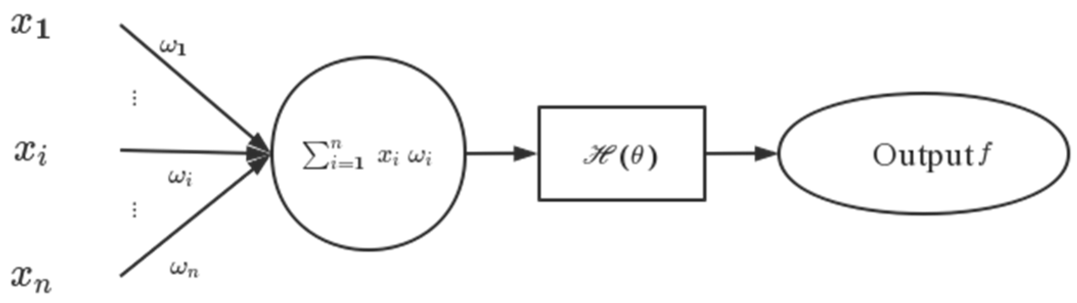
Neural network (NN) classification method

Neural networks utilize neural networks for classification by modeling the way the human nervous system works.

A neuron can be understood as a multi-dimensional linear function or a unit that achieves a linear combination. In the figure, $\left\{x\right\}$ is the input to the neuron, $\mathcal{H}\left(\theta \right)$ is the threshold function, and f represents the output.ω is the weights in the linear combination or the slope of the line. To facilitate the representation and computation of a considerable number of weights, they are typically represented as vectors or matrices.

The NN approach is shown in Figure 7:

NN is the current mainstream algorithm used for image classification, which supports automatic learning of features and patterns in the data and has good adaptability to non-linear relationships, Its computational units support highly paralleled computation, which speeds up the training speed, its distributed storage and processing improves the fault tolerance of the system, and it has a good generalization ability after sufficient training and is able to perform accurate classification on unseen data. When dealing with large-scale data and complex tasks, NN requires longer training time and more massive computational resources and can be improved in terms of reasonable choice of network structure, adjustment of hyper parameters, and avoidance of over-fitting to address the problem.

The categories, application directions, advantages, and disadvantages of the seven algorithms are compared in

Table 2. Comparison table of classification algorithms.

Methods	Categories	Application Scenarios	Advantages	Disadvantages
SVM	Supervised learning method	Classification and regression, text classification, image recognition	Adaptability of high-dimensional spatial data processing and small sample data processing	Less efficient processing of large data sets
XGBoost	Ensemble learning	Biclassification, multiclassification, and regression problems	High efficiency, flexibility, automatic selection of important features, prevention of overfitting, parallel computation	Less efficient processing of large data sets
Catboost	Ensemble learning	Biclassification, multiclassification, and regression problems	Strong ability of handling categorical features, robustness, high performance, GPU acceleration support, automatic feature selection, and friendly treatment of sparse data	Poor robustness of large-scale data and non-linear relationship processing
Adaboost	Ensemble learning	Biclassification, multiclassification, and regression problems	Easy to implement and adjust, not easy to overfit, combination with various basic classifiers	Noise sensitive
Random Forest	Ensemble learning	Image recognition, data prediction	Parallel processing, stable model, good generalization ability	Noise sensitive, long tree construction time, large memory consumption
LightGBM	Ensemble learning	Machine learning and data mining areas	Efficient, distributed structure, and high performance	Noise sensitive
Neural Network	Machine learning	Image classification, computer vision, natural language processing	High classification accuracy, strong parallel distributed processing, noise robustness	Extensive parameter adjustment, non-intuitive learning process, and long learning time

, which is shown underneath:

4. Experiments and the Results

This section describes the specific experimental process and methodology of the aero-engine classification experiment, which consists of three parts: aero-engines, spectral acquisition experimental design, data set production and spectral feature vector extraction, and classification prediction result accuracy assessment. Among them, the part of aero-engines spectral measurement experiment design describes the field arrangement of the aero-engine hot jet spectral measurement experiment, the part of data set fabrication and spectral feature vector extraction describes the training data set, test data set, label set production, and spectral feature vector extraction adopted in the classification experiment, and the classification prediction result accuracy assessment section evaluates the prediction of the classification method used in this paper on the real data set. Ultimately, the experimental result graphs and evaluation index tables are provided.

4.1. Experimental Design of Aero-Engine Spectral Measurement

In the first place, the infrared spectral data of three different aero-engines’ types were collected by field measurement. The FT-IR spectrometers used in the experiment are the EM27 and the telemetry FT-IR spectrometer developed by the Aerospace Information Research Institute. The specific parameters of the two devices are shown in

Table 3. Parameters of the Fourier transform infrared spectrometers used for the experiment.

Name	Manufacturer	Measurement Pattern	Spectral Resolution (cm−1)	Spectral Measurement Range (μm)	Full Field of View Angle
EM27	Bruker	Active/Passive	Active: 0.5/1 Passive: 0.5/1/4	2.5~12	30 mrad (no telescope) (1.7°)
Telemetry Fourier Transform Infrared Spectrometer	Aerospace Information Research Institute	Passive	1	2.5~12	1.5°

:

The experimental preparation stage requires the experimental devices to be set up according to the experimental conditions in the external field.

Initially, according to the spectrometers’ field of view angle and hot jet information, the measurement distance was adjusted with a telescope to ensure the hot jet fills the field of view. The EM27 and telemetry FT-IR spectrometer were mounted on two tripods, the laser and scopes were used to assist the aiming, and the height and angle of the tripod were adjusted so that the optical axis of the equipment was aligned with the center of the aero-engine tail nozzle.

Next, after fixing the position, increase the tripod counterweight to improve stability and fix the thermos-hygrometer near the measurement position. Determine the position of the infrared thermal camera to clearly photograph the hot jet to be measured.

Finally, the workstation display time and the control room control system time were strictly aligned. After the cooling process is finished, launch the two computer programs listed above in that order. In the EM27 program, adjust the measurement mode, spectral resolution, and number of superimposed cycles. Then, work with the displayed ADJUST value to adjust the tripod angle until the highest value is recorded. Following the completion of the settings, background data were collected from the spectrum during the times when the aero-engine was not running.

The layout of the experimental site is presented in Figure 8:

During the experiment, real-time communication was conducted with the person in charge of the aero-engine through walkie-talkies, requesting real-time prompts when the rotational speed was changed, and requesting that each test rotational speed be stabilized for 1 min as much as possible (since 100% rotational speed is difficult to be maintained for 1 min in the actual measurement process, the amount of spectral data collected in this part is small). The ambient temperature and humidity were recorded at each adjustment of the rotational speed. The environmental factors of the experiment were recorded as shown in

Table 4. Table of experimental aero-engines and environmental factors.

Aero-Engine Serial Number	Environmental Temperature	Environmental Humidity	Detection Distance
1	30 °C	43.5% Rh	11.8 m
2	20 °C	71.5% Rh	5 m
3	19 °C	73.5% Rh	10 m

:

Table 4 provides the conditions under which the experiment was carried out. The temperature and humidity in the environment cause an absorbing and attenuating effect on the spectrum, which responds to atmospheric radiative transfer. When solar radiation and surface thermal radiation are transmitted in the atmosphere, they are affected by the absorption and scattering of atmospheric molecules like H₂O, mixed gases (CO₂, CO, N₂O, CH₄, O₂), O₃, N₂, etc., on the one hand, and by the scattering or absorption of aerosolized particulate matter on the other hand, which results in the attenuation of the solar radiation and surface thermal radiation. At a distance from the target, the atmosphere will have a non-negligible effect on the collected spectrum. As of currently, we utilize the method of ground testing, the experimental distance is relatively close, and the difference between aero-engines’ hot jets and the background is very large, so the attenuation can be ignored.

4.2. Data Set Production and Spectral Feature Vectors Extraction

Based on the actual measurements of the aero-engines in the field, the controllable rotational speed ratios differed for each engine. Therefore, the infrared spectral data of 70%, 80%, 90%, and 100% of the maximum rotational speed ratios common to the three aero-engines were selected as the data source. There are a total of 211 spectral data in the data source, and after removing 2 erroneous data, 209 reliable data remain.

The experiment was conducted based on the aero-engine models, so the original data were divided by the aero-engines’ types. In the first place, 209 pieces of data were assigned random numbers from 1 to 209 to ensure the numbers were unrepeated, and the labels corresponding to the data were recorded (the labels corresponded to the engine model), 3/4 of them and their labels were selected at random as the training data set, and the rest of the data with the labels were used as the test data set.

The spectral features of the experimentally measured three aero-engines at 70%, 80%, 90%, and 100% of the maximum rotational speed were counted, and the statistical results were plotted as a two-dimensional feature map (as shown in the figure below), where the horizontal coordinates are $a_1$ and the vertical coordinates are $a_2$, as shown in Figure 9.

The aero-engines of the three aircraft are relatively sufficient for fuel combustion, and the exhaust gas spectrum at different speeds is close, so the gas composition characteristics of the gas discharged at the cruise speed of the three aircraft aero-engines are compared. Due to the various environment, temperature, and other conditions of the three field experiments, the spectrograms were compared after deducting the background. From the two-dimensional feature map, it can be regarded that the two-dimensional feature vectors of the three types of engines have been distributed in different regions of the feature space, and the overlap region between each other is relatively small, so the constructed spectral feature vectors initially have the ability to classify.

The spectral feature vectors and the classifier are combined to train and predict the spectral data. The flow chart of the classification algorithm used in the experiment is shown in Figure 10:

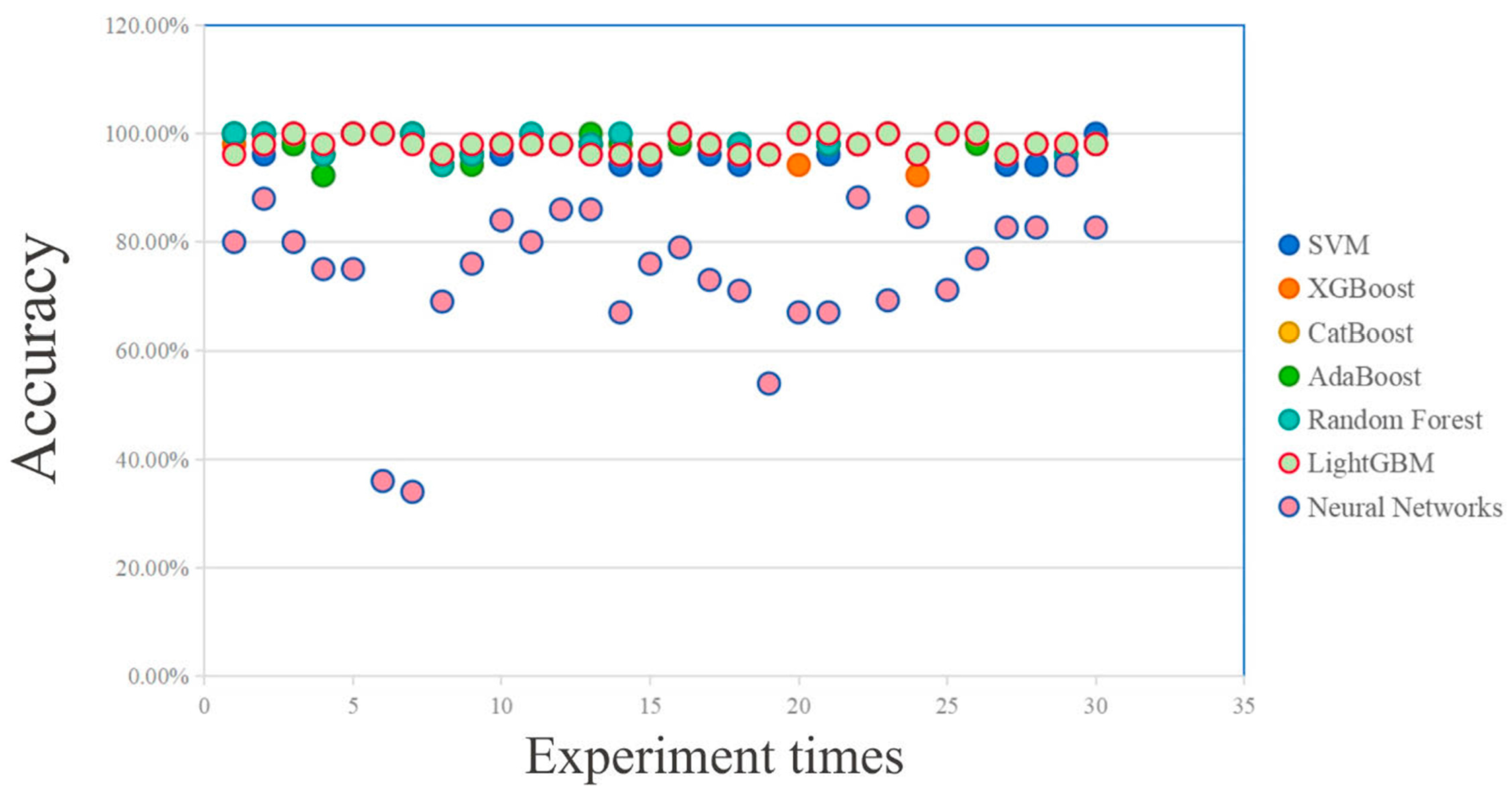
4.3. Assessment of the Accuracy of Classification Prediction Results

The experimentally constructed infrared spectra training data set and test data set are tested for classification of spectral feature vectors with seven classifiers, SVM, XGBoost, CatBoost, AdaBoost, Random Forest, LightGBM, and neural networks, and the classification results are shown in Figure 11:

Where, red, green, and blue represent the feature vectors of the three correctly classified aero-engine hot jet infrared spectra, while black represents the misclassified feature vectors.

At the same time, the parameters of the seven classification algorithms are given in

Table 5. Parameter list of classification algorithms.

Methods	Parameter Settings
SVM	decision_function_shape = ‘ovr’, kernel = ‘rbf’
XGBoost	objective = ‘multi:softmax’, num_classes = num_classes
CatBoost	loss_function = ‘MultiClass’
Adaboost	n_estimators = 200
Random Forest	n_estimators = 300
LightGBM	objective’: ‘multiclass’, ‘num_class’: num_classes
Neural Network	hidden_layer_sizes = (100), activation = ‘relu’, solver = ‘adam’, max_iter = 200

, which is shown below:

The evaluation criteria for aero-engine spectral classification consist of accuracy, precision, recall, F1 value (F1-score), and confusion matrix [26]. It is assumed that if the instance is a positive class and is predicted to be positive, i.e., true class, it is denoted as TP (true positive), and if it is predicted to be negative, i.e., false negative, it is denoted as FN (false negative); on the contrary, if the instance is a negative class and it is predicted to be positive, i.e., false positive, it is denoted as FP (false positive), and if it is predicted to be negative, i.e., true negative, it is denoted as TN (true negative). Based on the above assumptions, the accuracy, precision, recall, F1 value, and confusion matrix of the evaluation criteria are defined separately:

① Accuracy: proportion of correctly categorized samples to total samples.

$$\mathrm{Accuracy} =\frac{\mathrm{T}\mathrm{P}+\mathrm{T}\mathrm{N}}{\mathrm{T}\mathrm{P}+\mathrm{T}\mathrm{N}+\mathrm{F}\mathrm{P}+\mathrm{F}\mathrm{N}}$$

(23)

② Precision: the ratio of the number of samples correctly predicted to be positive to the number of all samples predicted to be positive.

$$\mathrm{Precision} =\frac{\mathrm{T}\mathrm{P}}{\mathrm{T}\mathrm{P}+\mathrm{F}\mathrm{P}}$$

(24)

③ Recall: the ratio of the number of samples correctly predicted to be in the positive category to the number of samples in the true positive category.

$$\mathrm{Recall} =\frac{\mathrm{T}\mathrm{P}}{\mathrm{T}\mathrm{P}+\mathrm{F}\mathrm{N}}$$

(25)

④ F1-score: the F1 value combines the harmonic mean of precision and recall and is used to measure the overall performance of the model.

$$\mathrm{F}1-\mathrm{score} =\frac{2^{*}{P}^{*}R}{P+R}$$

(26)

Among them, $P$ represents Precision, $R$ represents Recall.

⑤ Confusion matrix: The confusion matrix shows how well the classifier categorized the different categories, including true examples, false positive examples, true negative examples, and false negative examples. It proves the difference between the actual and predicted values, and the values on the diagonal of the confusion matrix indicate the number of correct predictions made by the classifier for that category. The confusion matrix is shown in

Table 6. Confusion matrix.

		Forecast Results
		Positive samples	Negative samples
Real results	Positive samples	TP	TN
	Negative samples	FP	FN

:

According to the above five evaluation criteria for the algorithm of combining spectral feature vectors and classifiers used in this paper to predict the labels of the prediction set, the prediction results are shown in

Table 7. Table of classification and evaluation indexes of aero-engine hot jet infrared spectrum feature vectors and seven classifier algorithms.

	Evaluation Criterion	Accuracy	Precision Score	Recall	F1	Confusion Matrix	Running Time/s
Classification Methods
feature vectors + SVM		98.04%	98.77%	97.78%	98.22%	$\left[\begin{array}{ccc}26& 0& 0\\ 0& 10& 0\\ 1& 0& 14\end{array}\right]$	2.48
Feature vectors + XGBoost		98.04%	98.77%	97.78%	98.22%	$\left[\begin{array}{ccc}26& 0& 0\\ 0& 10& 0\\ 1& 0& 14\end{array}\right]$	2.62
Feature vectors + CatBoost		98.04%	98.77%	97.78%	98.22%	$\left[\begin{array}{ccc}26& 0& 0\\ 0& 10& 0\\ 1& 0& 14\end{array}\right]$	5.27
Feature vectors + AdaBoost		98.04%	98.77%	97.78%	98.22%	$\left[\begin{array}{ccc}26& 0& 0\\ 0& 10& 0\\ 1& 0& 14\end{array}\right]$	2.91
Feature vectors + Random Forest		98.04%	98.77%	97.78%	98.22%	$\left[\begin{array}{ccc}26& 0& 0\\ 0& 10& 0\\ 1& 0& 14\end{array}\right]$	3.09
Feature vectors + LightGBM		96.08%	96.38%	96.38%	96.38%	$\left[\begin{array}{ccc}26& 0& 1\\ 0& 10& 0\\ 1& 0& 13\end{array}\right]$	2.63
Feature vectors + Neural Networks		80.39%	76.19%	90.99%	76.27%	$\left[\begin{array}{ccc}27& 0& 10\\ 0& 10& 0\\ 0& 0& 4\end{array}\right]$	2.41

:

The evaluation criteria for combining the aero-engine hot jet infrared spectral feature vectors with the seven classifier combination algorithms are analyzed according to the preceding table. Since the experimental data set is generated by random numbering based on the experimental measurement spectra, the probability of predicting the data possesses a certain degree of chance. Therefore, several experiments were conducted to evaluate the general accuracy, and the correctness is shown in Figure 12, where the data of CatBoost (shown yellow) basically overlaps with AdaBoost.

The data from the 30 experiments conducted were counted to obtain the classifier prediction probability statistics as shown in

Table 8. Statistics of prediction probability of classifiers.

Method Order	SVM	XGBoost	CatBoost	AdaBoost	Random Forest	LightGBM	Neural Networks
Average value	97.17%	97.74%	98.13%	98.00%	98.32%	98.07%	74.52%
Variance	0.06%	0.04%	0.03%	0.04%	0.03%	0.02%	1.84%
Standard deviation	2.41%	1.96%	1.71%	1.92%	1.73%	1.52%	13.56%

:

According to Table 8, in terms of accuracy, CatBoost, AdaBoost, Random Forest, and LightGBM in repeated experiments maintain good accuracy and can achieve relatively accurate prediction in multiple experiments. The prediction accuracy of SVM is average, while the performance of neural networks is unsatisfactory. In terms of time measures, the seven methods have a similar running time, while CatBoost is slightly slower. Substantially, the mainstream classifiers have achieved a relatively ideal classification accuracy.

5. Conclusions

In this paper, for the aero-engine classification problem, two Fourier transform infrared spectrometers, Bruker’s EM27 and self-developed telemetry FT-IR spectrometer, were used to telemetry the infrared spectra of the hot jet of three aero-engine engines in different states, the training data set and test data set were randomly divided in the ratio of 3:1, and the spectral feature vectors were used to combine with the classification algorithm for the training of the training data set and the labeling of the test set. The classification evaluation indexes are accuracy, precision, recall, confusion matrix, and F1-score, and the classification accuracy of the algorithm is about 98%.

The spectral feature vectors proposed in this paper remain a preliminary concept for the aero-engine classification and identification problem, and in the subsequent stage, we will further study the infrared radiation model of the aero-engines’ hot jet and statistically analyze the more stable feature peaks in the infrared spectrum of the hot jet to find out the most stable feature peaks to build more robust spectral feature vectors, which can be used for more accurate classification of the aero-engines; furthermore, the spectral feature vectors proposed in this paper can be used for more accurate classification of the aero-engines. Expand the hot jet infrared spectral data of aero-engines and try using the measured spectral data to expand the aero-engine hot jet infrared spectral library, so as to develop a foundation for the recognition of aero-engines; under the premise of insufficient data, the method of deep migration learning can be introduced to expand the amount of training samples, so as to improve the training degree of the model.

References

1. Razeghi, M.; Nguyen, B.M. Advances in mid-infrared detection and imaging: A key issues review. Rep. Prog. Phys. 2014, 77, 082401. [Google Scholar] [CrossRef]
2. Chikkaraddy, R.; Arul, R.; Jakob, L.A.; Baumberg, J.J. Single-molecule mid-IR detection through vibration ally-assisted luminescence. arXiv 2022, arXiv:2205.07792. [Google Scholar]
3. Knez, D.; Toulson, B.W.; Chen, A.; Ettenberg, M.H.; Nguyen, H.; Potma, E.O.; Fishman, D.A. Spectral imaging at high definition and high speed in the mid-infrared. Sci. Adv. 2022, 8, eade4247. [Google Scholar] [CrossRef]
4. Zhang, J.; Gong, Y. Automated identification of infrared spectra of hazardous clouds by passive FTIR remote sensing. In Multispectral and Hyperspectral Image Acquisition and Processing; SPIE: Bellingham, DC, USA, 2001; Volume 4548, pp. 356–362. [Google Scholar]
5. Roh, S.B.; Oh, S.K. Identification of Plastic Wastes by Using Fuzzy Radial Basis Function Neural Networks Classifier with Conditional Fuzzy C-Means Clustering. J. Electr. Eng. Technol. 2016, 11, 103–116. [Google Scholar] [CrossRef]
6. Kumar, V.; Kashyap, M.; Gautam, S.; Shukla, P.; Joshi, K.B.; Vinayak, V. Fast Fourier infrared spectroscopy to characterize the biochemical composition in diatoms. J. Biosci. 2018, 43, 717–729. [Google Scholar] [CrossRef]
7. Han, X.; Li, X.; Gao, M.; Tong, J.; Wei, X.; Li, S.; Ye, S.; Li, Y. Emissions of Airport Monitoring with Solar Occultation Flux-Fourier Transform Infrared Spectrometer. J. Spectrosc. 2018, 2018, 1069612. [Google Scholar] [CrossRef]
8. Cięszczyk, S. Passive Open-Path FTIR Measurements and Spectral Interpretations for in situ Gas Monitoring and Process Diagnostics. Acta Phys. Pol. A 2014, 126, 673–678. [Google Scholar] [CrossRef]
9. Schütze, C.; Lau, S.; Reiche, N.; Sauer, U.; Borsdorf, H.; Dietrich, P. Ground-based remote sensing with open-path Fourier-transform infrared (OP-FTIR) spec-troscopy for large-scale monitoring of greenhouse gases. Energy Procedia 2013, 37, 4276–4282. [Google Scholar] [CrossRef]
10. Doubenskaia, M.; Pavlov, M.; Grigoriev, S.; Smurov, I. Definition of brightness temperature and restoration of true temperature in laser cladding using infrared camera. Surf. Coat. Technol. 2013, 220, 244–247. [Google Scholar] [CrossRef]
11. Homan, D.C.; Cohen, M.H.; Hovatta, T.; Kellermann, K.I.; Kovalev, Y.Y.; Lister, M.L.; Popkov, A.V.; Pushkarev, A.B.; Ros, E.; Savolainen, T. MOJAVE. XIX. Brightness Temperatures and Intrinsic Properties of Blazar Jets. Astrophys. J. 2021, 923, 67. [Google Scholar] [CrossRef]
12. Schumann, U. On the effect of emissions from aircraft engines on the state of the atmosphere. Ann. Geophys. 2005, 12, 365–384. [Google Scholar] [CrossRef]
13. Boser, B.E.; Guyon, I.M.; Vapnik, V.N. A training algorithm for optimal margin classifiers. In Proceedings of the Fifth Annual Workshop on Computational Learning Theory, Pittsburgh, PA, USA, 27–29 July 1992; pp. 144–152. [Google Scholar]
14. Zhang, Y.; Li, T. Three different SVM classification models in Tea Oil FTIR Application Research in Adulteration Detection. J. Phys. Conf. Ser. 2021, 1748, 022037. [Google Scholar] [CrossRef]
15. Menezes, M.V.; Torres, L.C.; Braga, A.P. Width optimization of RBF kernels for binary classification of support vector machines: A density estimation-based approach. Pattern Recognit. Lett. 2019, 128, 1–7. [Google Scholar] [CrossRef]
16. Chen, T.; Guestrin, C. XGBoost: A scalable tree boosting system. In Proceedings of the 22nd ACM SIGKDD International Conference on Knowledge Discovery and Data Mining, San Francisco, CA, USA, 13–17 August 2016; pp. 785–794. [Google Scholar]
17. Nalluri, M.; Pentela, M.; Eluri, N.R. A Scalable Tree Boosting System: XGBoost. Int. J. Res. Stud. Sci. Eng. Technol. 2020, 7, 36–51. [Google Scholar]
18. Prokhorenkova, L.; Gusev, G.; Vorobev, A.; Dorogush, A.V.; Gulin, A. CatBoost: Unbiased boosting with categorical features. arXiv 2018, arXiv:1706.09516. [Google Scholar]
19. Dorogush, A.V.; Ershov, V.; Gulin, A. CatBoost: Gradient boosting with categorical features support. arXiv 2018, arXiv:1810.11363. [Google Scholar]
20. Dorogush, A.V.; Gulin, A.; Gusev, G.; Kazeev, N.; Prokhorenkova, L.O.; Vorobev, A. Fighting biases with dynamic boosting. arXiv 2017, arXiv:1706.09516. [Google Scholar]
21. Freund, Y.; Schapire, R.; Abe, N. A short introduction to boosting. J.-Jpn. Soc. Artif. Intell. 1999, 14, 771–780. [Google Scholar]
22. Breiman, L. Random Forests. Mach. Learn. 2001, 45, 5–32. [Google Scholar] [CrossRef]
23. Ke, G.; Meng, Q.; Finley, T.; Wang, T.; Chen, W.; Ma, W.; Ye, Q.; Liu, T.Y. Lightgbm: A highly efficient gradient boosting decision tree. Adv. Neural Inf. Proc. Syst. 2017, 30, 3149–3157. [Google Scholar]
24. Zeng, P. Artificial Neural Networks Principle for Finite Element Method. Z. Angew. Math. Mech. 1996, 76, 565–566. [Google Scholar]
25. ArulRaj, K.; Karthikeyan, M.; Narmatha, D. A View of Artificial Neural Network Models in Different Application Areas. E3S Web Conf. 2021, 287, 03001. [Google Scholar] [CrossRef]
26. Sokolova, M.; Lapalme, G. A systematic analysis of performance measures for classification tasks. Inf. Proc. Manag. 2009, 45, 427–437. [Google Scholar] [CrossRef]
Figure 1. Experimentally measured hot jets’ infrared spectra of three turbojet engines.
Electronics 13 00915 g001
Figure 2. Schematic representation of the positions of the four characteristic peaks of the three aero-engines as measured in practice.
Electronics 13 00915 g002
Figure 3. Schematic representation of dichotomy SVM data classification.
Electronics 13 00915 g003
Figure 4. Schematic representation of the AdaBoost algorithm.
Electronics 13 00915 g004
Figure 5. Schematic representation of the LightGBM algorithm.
Electronics 13 00915 g005
Figure 6. Schematic representation of the RF algorithm.
Electronics 13 00915 g006
Figure 7. Schematic representation of the NN algorithm.
Electronics 13 00915 g007
Figure 8. Schematic representation of the aero-engine hot jet infrared spectrum measurement experiment site.
Electronics 13 00915 g008
Figure 9. Characteristic statistical results of three different turbojet aero-engines at 70%, 80%, 90%, and 100% maximum speed.
Electronics 13 00915 g009
Figure 10. Flowchart of the spectral feature vector aero-engine classification algorithm.
Electronics 13 00915 g010
Figure 11. Aero-engine hot jet infrared spectral feature vector classification effect map.
Electronics 13 00915 g011aElectronics 13 00915 g011bElectronics 13 00915 g011c
Figure 12. Distribution of correct rates for each algorithm under 30 experiments.
Electronics 13 00915 g012