Efficient Vision Transformer YOLOv5 for Accurate and Fast Traffic Sign Detection

Abstract

Accurate and fast detection of traffic sign information is vital for autonomous driving systems. However, the YOLOv5 algorithm faces challenges with low accuracy and slow detection when it is used for traffic sign detection. To address these shortcomings, this paper introduces an accurate and fast traffic sign detection algorithm–YOLOv5-Efficient Vision TransFormer(EfficientViT)). The algorithm focuses on improving both the accuracy and speed of the model by replacing the CSPDarknet backbone of the YOLOv5(s) model with the EfficientViT network. Additionally, the algorithm incorporates the Convolutional Block Attention Module(CBAM) attention mechanism to enhance feature layer information extraction and boost the accuracy of the detection algorithm. To mitigate the adverse effects of low-quality labels on gradient generation and enhance the competitiveness of high-quality anchor frames, a superior gradient gain allocation strategy is employed. Furthermore, the strategy introduces the Wise-IoU (WIoU), a dynamic non-monotonic focusing mechanism for bounding box loss, to further enhance the accuracy and speed of the object detection algorithm. The algorithm’s effectiveness is validated through experiments conducted on the 3L-TT100K traffic sign dataset, showcasing a mean average precision (mAP) of 94.1% in traffic sign detection. This mAP surpasses the performance of the YOLOv5(s) algorithm by 4.76% and outperforms the baseline algorithm. Additionally, the algorithm achieves a detection speed of 62.50 frames per second, which is much better than the baseline algorithm.

1. Introduction

A crucial component of autonomous driving is the accurate and fast detection of traffic signs [1]. The recognition of traffic signs is a deep learning-based procedure where the detection algorithm learns from labeled signage data to extract important information about the signage. The causes of 94% of these incidents, including human mistake and inattentive driving, can be eliminated with autonomous vehicles [2]. Traffic accidents caused by self-driving cars that are traveling too fast and lack information from signage for decision-making judgement can be avoided by accurate and fast object detection algorithms that capture signage information.

Deep learning-based traffic sign detection algorithms, shape-based traffic sign detection algorithms, and color-based traffic sign detection algorithms are the three basic types of traffic sign detection algorithms [3,4]. For instance, one technique uses color features to separate traffic signs by assessing color variances between the signs and the surrounding environment and defining color thresholds [5]. However, weather and lighting changes might affect color-based techniques. Yakimov et al. use the Hough transform technique to identify traffic signs based on their distinct shapes. However, when signs are partially hidden, this shape-based strategy is useless [6]. Balali et al. present a fusion strategy that uses both color and form features in order to overcome the shortcomings of the aforementioned methods. In comparison to applying each characteristic independently, the combination of these factors improves detection performance [7]. However, multi-feature fusion-based traffic sign recognition algorithms run into issues like the inability to recognize connected traffic signs and subpar real-time performance.

Driven by the advancements in deep learning detection algorithms, traffic sign detection algorithms have emerged as a powerful tool for extracting meaningful semantic information from images using convolutional neural networks. These algorithms leverage various detection frameworks to extract precise location and category information of traffic signs. Broadly speaking, deep learning traffic sign detection algorithms can be categorized into two types: two-stage region proposal (Two-Stage) and single-stage regression algorithm (One-Stage) [8,9]. Two-stage algorithms, such as R-CNN, Fast R-CNN, and Faster R-CNN, typically exhibit higher detection accuracy but slower speed [10,11,12]. Conversely, single-stage algorithms, including SSD [13], RetinaNet [14], and YOLO series [15,16,17], treat localization and classification as a regression problem, enabling end-to-end detection with faster processing but comparatively lower detection accuracy.

With the growth of migration learning, it has become popular to integrate a transformer model into the field of vision in order to address the issues of low detection accuracy and slow detection speed of existing detection algorithms [18]. The Vision Transformer (ViT) proposal demonstrates the value of the transformer paradigm in the realm of vision [19]. The ViT model resolves the issue that convolutional networks are unable to extract information about the global feature layer order and content, considerably enhancing the precision of detection algorithms. A unique lightweight multi-scale attention technique is used in the semantic segmentation model called the Efficient Vision Transformer (EfficientViT) [20]. The issue of the ViT model’s big parameters and slow speed is resolved by the EfficientViT, which also enhances the detection algorithm’s accuracy and speed in real time.

The mian contribution of this study is summarized as follows: (1) An EfficientViT network is designed as the backbone of YOLOv5 to improve the accuracy and speed of traffic sign detection. (2) The feature pyramid component’s incorporation of the CBAM attention mechanism, which enables the feature map to self-correct, suppresses irrelevant noise input and improves detection accuracy. (3) Making use of the WIoU (Wise IoU) bounding box loss function, which prioritizes crucial image features, mutes pointless regional replies and enhances the detection network’s overall performance.

The rest of the paper is structured as follows: The EffcientVit network’s fundamental structure, the attention mechanism, and information on the bounding box loss function are all introduced in Section 2. The experimental design and the experimental structure assessment index are introduced in Section 3. The experimental results and analysis are presented in Section 4. Finally, the conclusion is given in Section 5.

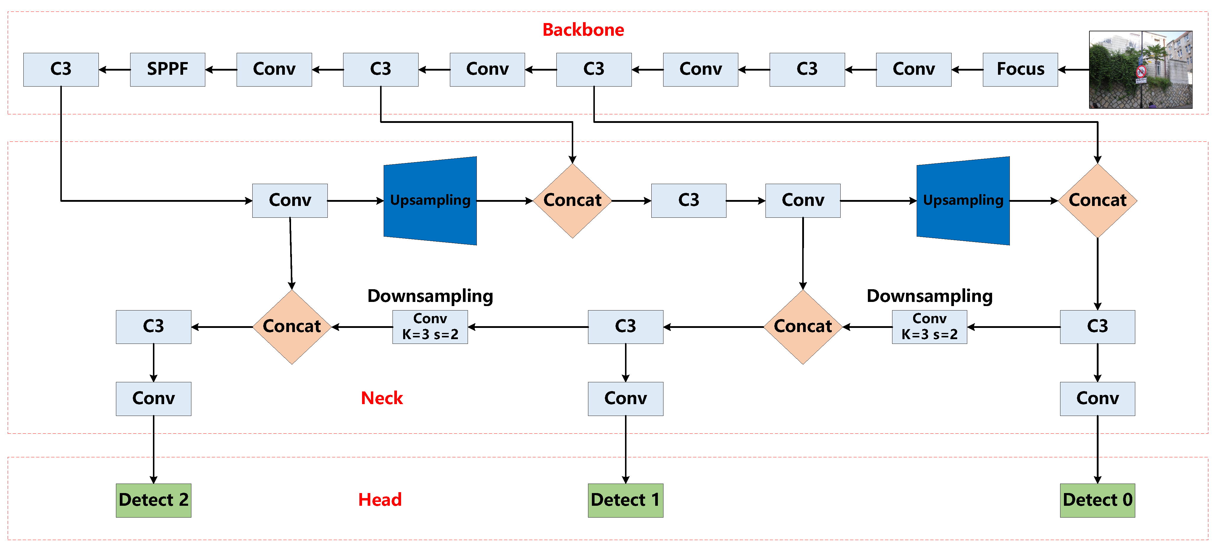
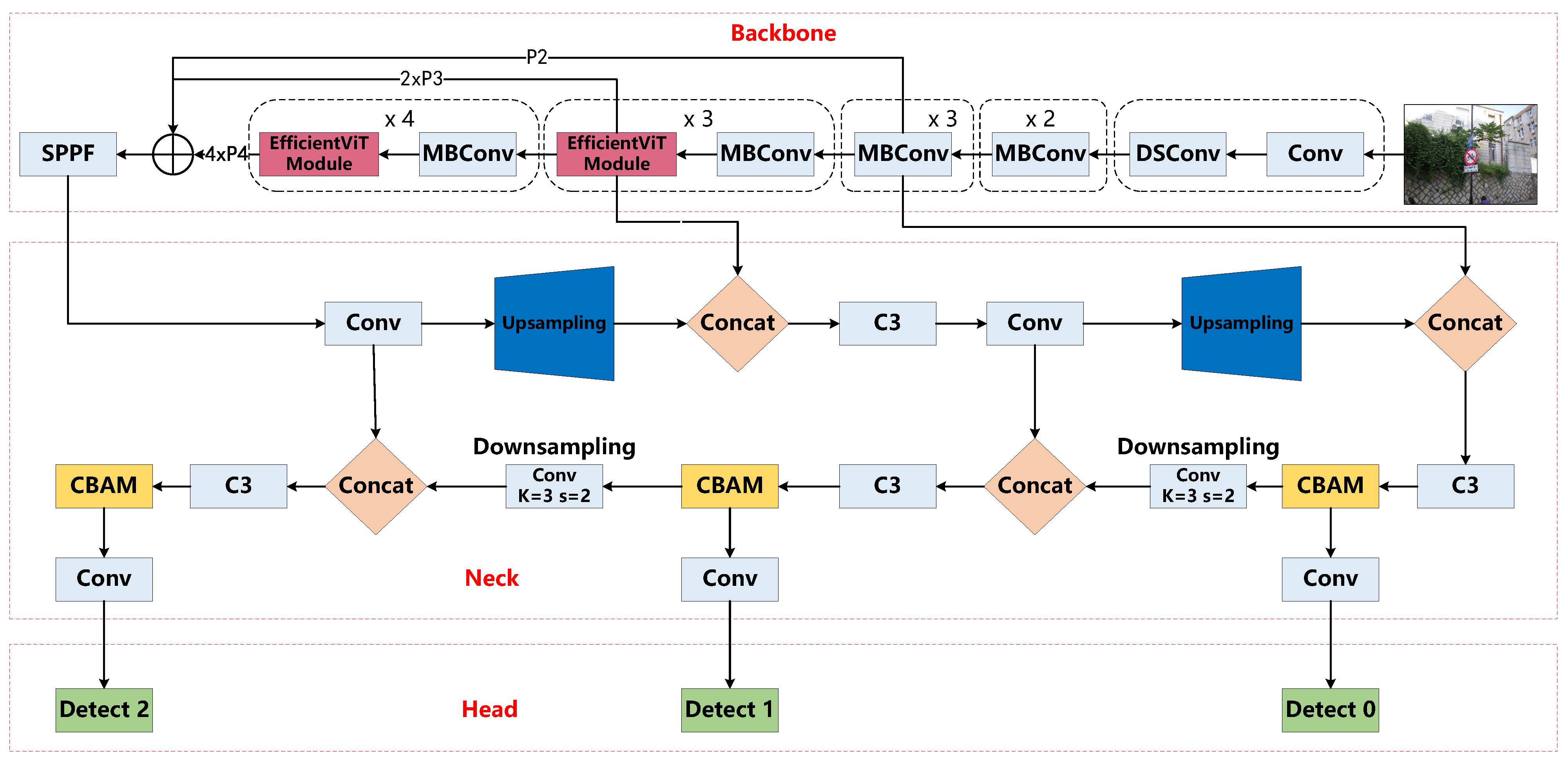
2. The YOLOv5-EfficinetViT Traffic Sign Detection Algorithm’s General Framework

Four primary components make up the YOLOv5(s) algorithm: input, backbone network (Backbone), neck, and head. The Focus, Conv, CSP, and SPPF networks make up the majority of the backbone network. The Focus structure separates the input image into 16 identically sized blocks, then joins the blocks to create four identical images for additional processing. The CSP network divides the input into two sections, stacking the remaining blocks in the first and performing extra operations in the second. The 5 × 5 MaxPool layers are successively applied to the input by the SPPF structure, which then sums the computed values from each layer. The output is then generated using a Conv+BN+Relu structure. Figure 1 shows how YOLOv5(s) is structured.

The YOLOv5-EfficientViT traffic sign detection algorithm presented in this paper is shown in Figure 2. The algorithm adds three crucial parts for a better performance. First off, a more effective extraction of traffic sign features is made possible by the EfficientViT network, which takes the place of the original YOLOv5 backbone CSPDarkNet network. Second, the CBAM attention mechanism improves the FPN structure by adding more refined characteristics and a stronger emphasis on non-noise information. Last but not least, the algorithm integrates the dynamic non-monotonic focusing mechanism known as the Wise IoU module to address the complementing balance between better and worse quality samples in the CIoU bounding frame loss function.

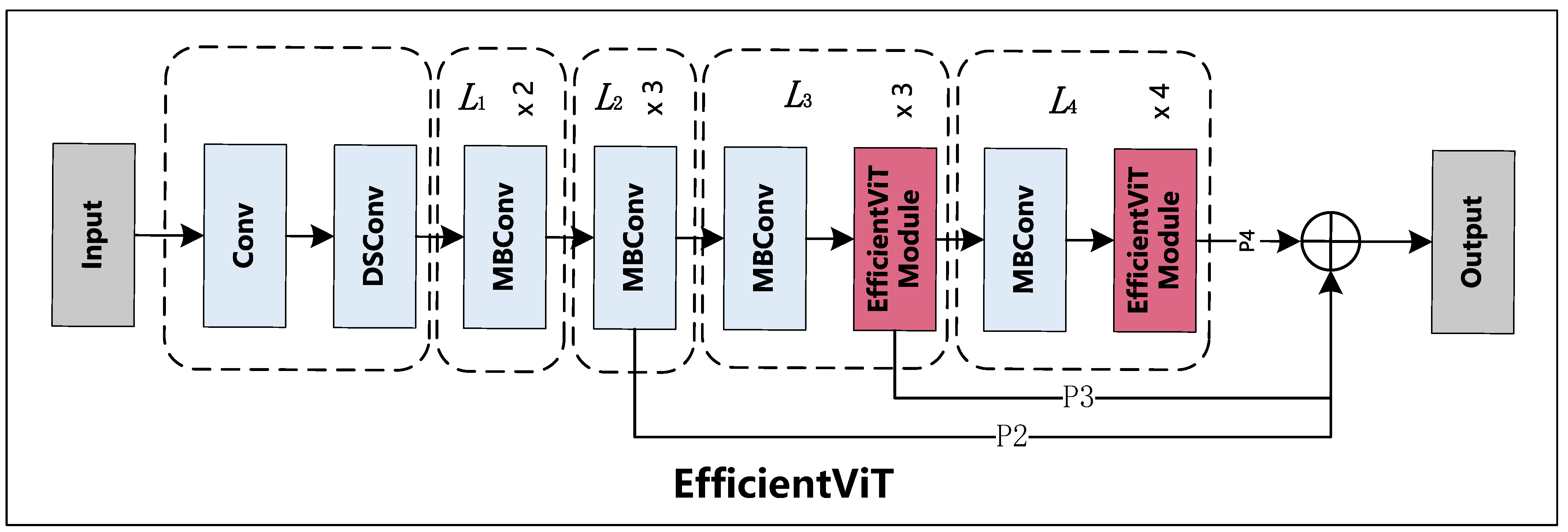
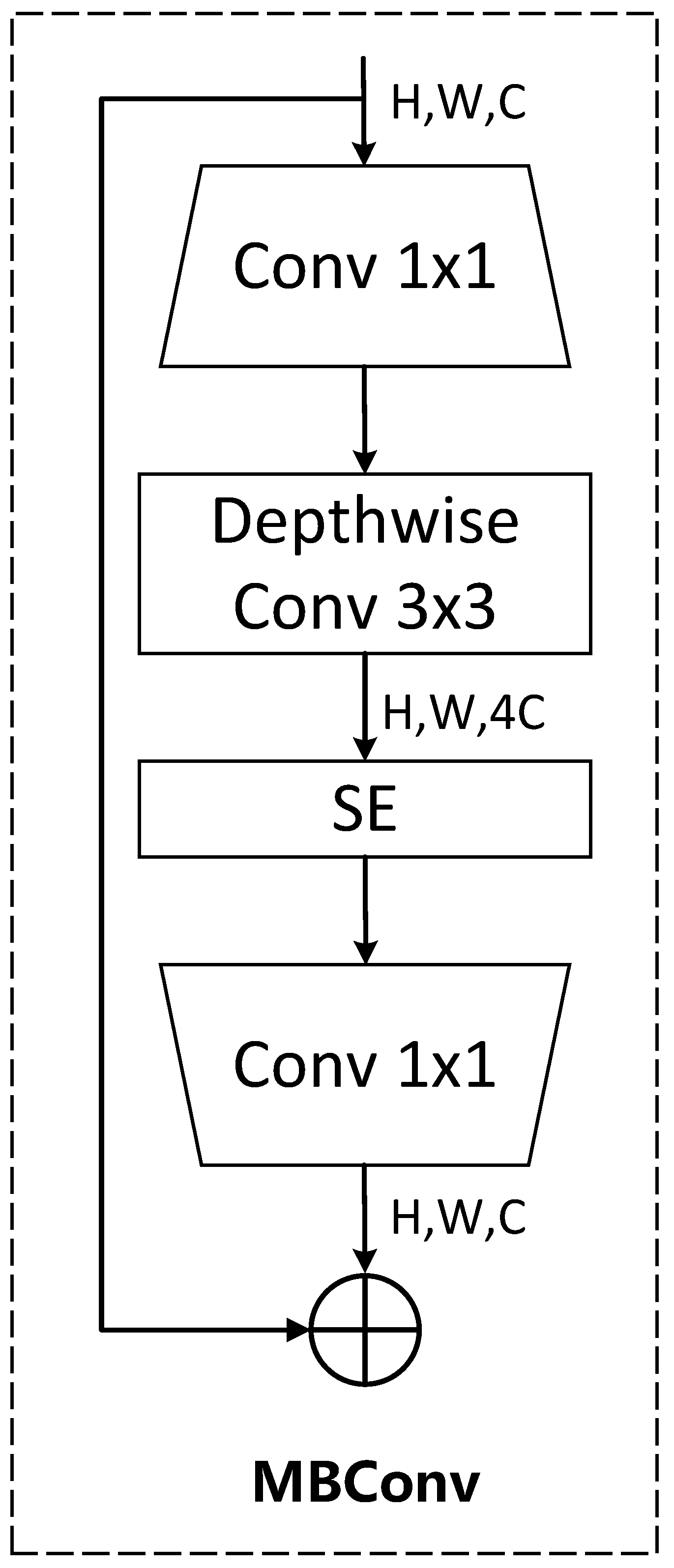
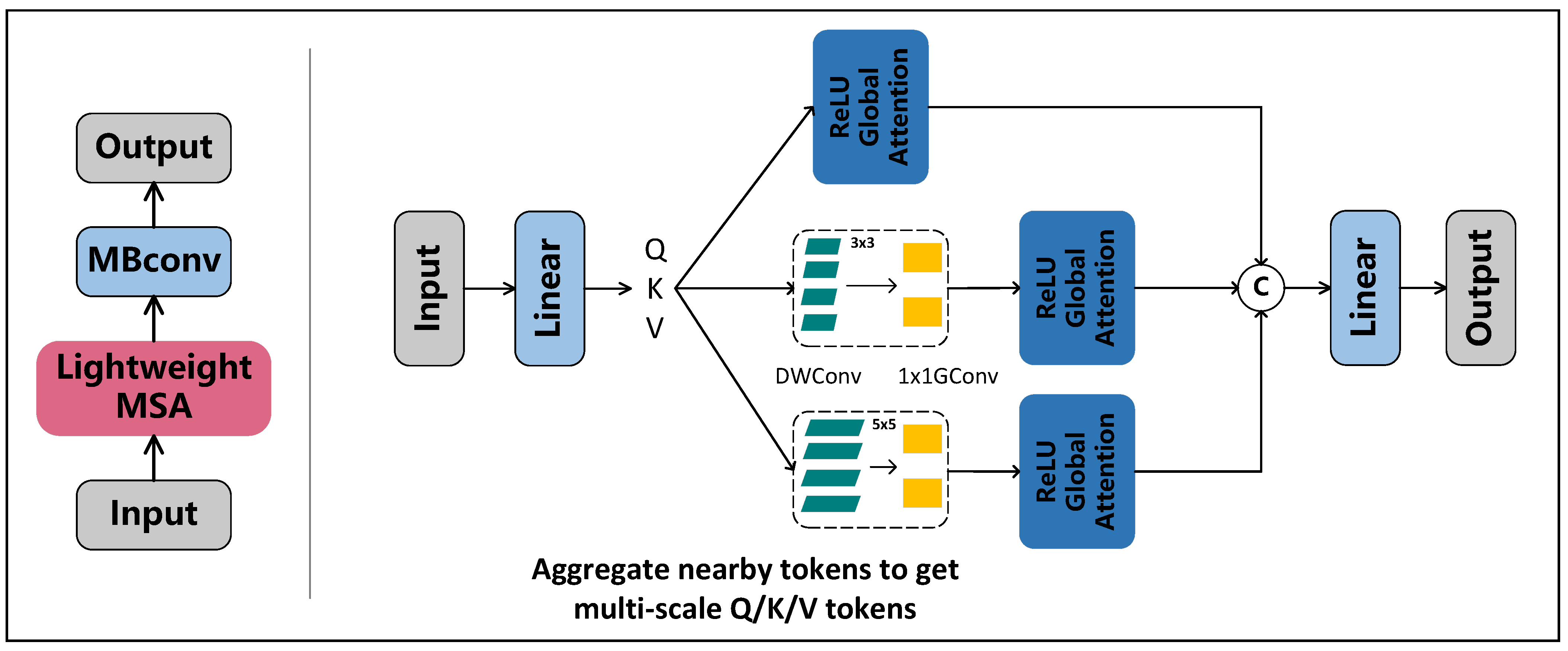
2.1. EfficientViT Backbone

The Vision TransFormer (ViT) architecture serves as the foundation for the image categorization model known as EfficientViT. The DSConv structure, MBConv structure, and EfficientViT module structure are only a few of the structures that this model comprises. The full structure of EfficientViT is shown in Figure 3.

The model first inputs the image and uses a convolution layer (Conv) to perform feature extraction and dimensionality reduction procedures. The output is placed via a depthwise separable convolution (DSConv) structure to boost performance and efficiency. The point-by-point convolution convolves the depthwise convolution output with a 1 × 1 convolution kernel to produce the final output feature map, whereas the depthwise convolution just conducts convolutions within each channel. This strategy maintains computational economy while improving the model’s performance.

The MBConv network processes the DSConv output twice, using the L1 layer and the L2 layer for feature extraction to obtain the P2 feature layer. The lightweight Inverted Residual Bottleneck (MBConv) architecture that serves as the foundation of the MBConv network starts with a 1 × 1 convolution. The SE (squeeze-and-excitation) module is also incorporated into the MBConv module to increase the relevance of features and improve the model’s overall performance. For a graphic illustration of the MBConv structure, please see Figure 4.

Two MBConv modules are incorporated into the EfficientViT model to create a P2 feature layer. The L3 EfficientViT module structure and one MBConv module are then applied to this P2 feature layer to produce the P3 feature layer. The input image and its features go through dimensionality leveling using a linear layer inside the EfficientViT module structure. Three containers $(Q/K/V)$ with an equal distribution of the data are used for three parallel operations. In the first operation, feature representation and information fusion are immediately implemented using the global attention mechanism with ReLU activation. In order to handle data about graph structure, the second operation first performs a deep convolution operation using a 3 × 3 kernel. The output is then activated by ReLU and sent into the global attention mechanism. The third step, which processes data about graph structure, includes a deep convolution operation with a 5 × 5 kernel, followed by graph convolution. The output is then inputted with ReLU activation into the global attention mechanism. The three parallel processes’ outputs are merged and stitched together, and the finished product is then run through a linear layer. Finally, the output’s dimensional representation is recovered by using the MBConv structure. Figure 5’s representation of the EfficientViT module structure shows a network of self-attentive mechanisms.

The input to the Relu-based global attention is $x\in {\mathbb{R}}^{N\times f}$, and the generalized self-attention mechanism is formulated as follows:

$$O_i=\sum _{j=1}^N\frac{\mathit{Sim}\left(Q_i,K_i\right)}{{\sum }_{j=1}^N\mathit{Sim}\left(Q_i,K_i\right)}{V}_j$$

(1)

where $Q=x{W}_Q$, $K=x{W}_K$, $V=x{W}_V$, and $W_Q/W_K/W_V\in {\mathbb{R}}^{f\times d}$ is the linear projection matrix, and $O_i$ denotes the ith row of matrix $Sim(.,.)$, which is the similarity function. When using the similarity function $Sim(Q,K)=exp\left(\frac{Q{K}^T}{\sqrt{d}}\right)$, Equation (1) is the original self-attention mechanism.

$$Sim(Q,K)=ReLU\left(Q\right)ReLU{\left(K\right)}^T$$

(2)

With $Sim(Q,K)=ReLU\left(Q\right)ReLU{\left(K\right)}^T$, Equation (1) can be rewritten as follows:

$$\begin{array}{c}\hfill Q_i=\sum _{j=1}^N\frac{\mathit{ReLU}\left(Q_i\right)\mathit{ReLU}{\left(K_j\right)}^T}{{\sum }_{j=1}^N\mathit{ReLU}\left(Q_i\right)\mathit{ReLU}{\left(K_j\right)}^T}{V}_j=\frac{{\sum }_{j=1}^N\left(\mathit{ReLU}\left(Q_i\right)\mathit{ReLU}{\left(K_j\right)}^T\right)V_j}{\mathit{ReLU}\left(Q_i\right){\sum }_{j=1}^N\mathit{ReLU}{\left(K_j\right)}^T}\end{array}$$

(3)

The L4 EfficientViT module structure processes the P3 special layer after it has been input into an MBConv module, resulting in the derivation of the P4 feature layer. The P4 broad dimension is extended using a multiplication factor of 4, whereas the P3 wide dimension is expanded using a factor of 2. The P2, P3, and P4 feature layers are additionally concatenated, and the resulting cumulative outputs are then fed into L5 MBConv modules for convolutional processing, producing the final output feature layer.

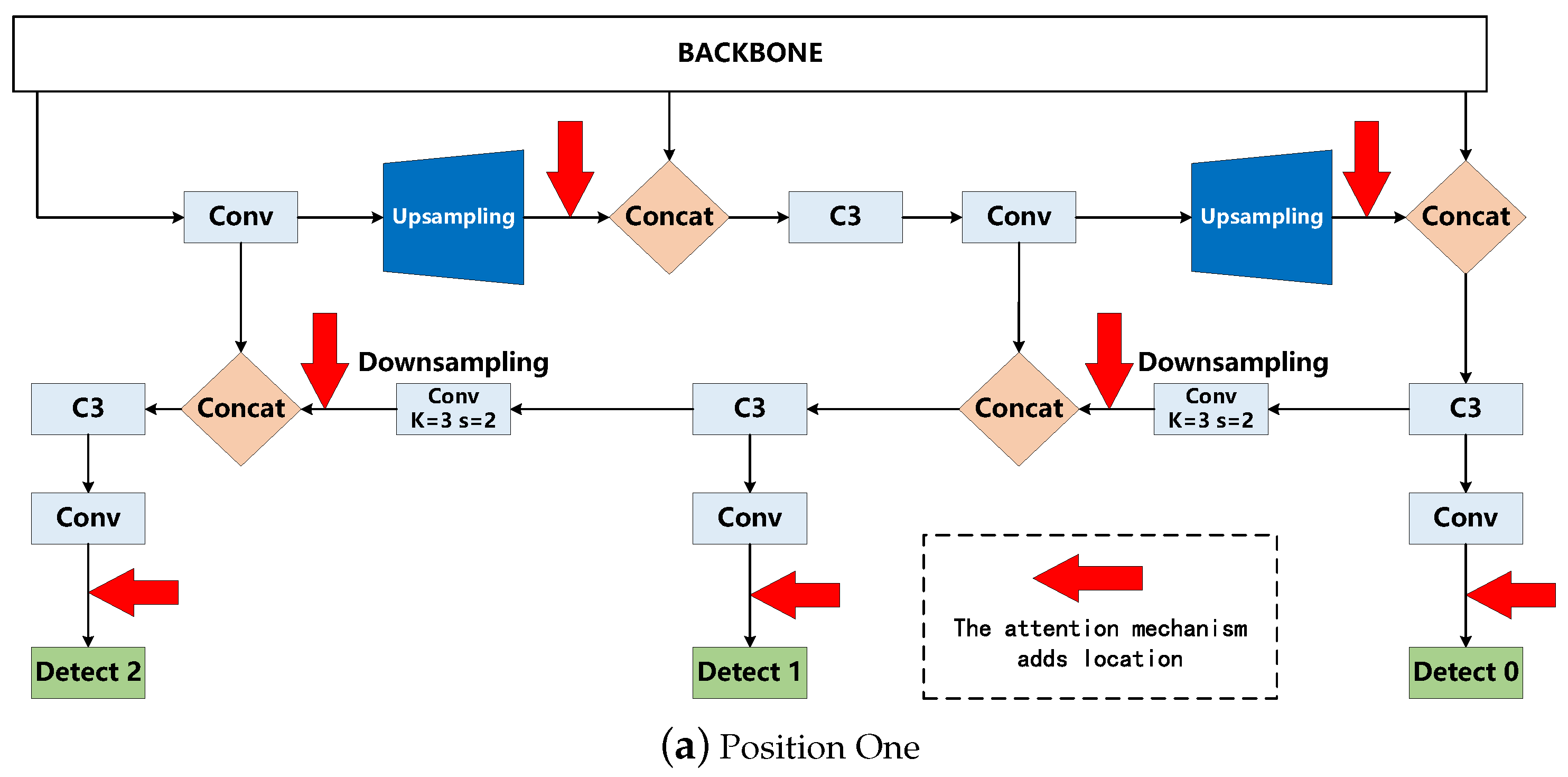
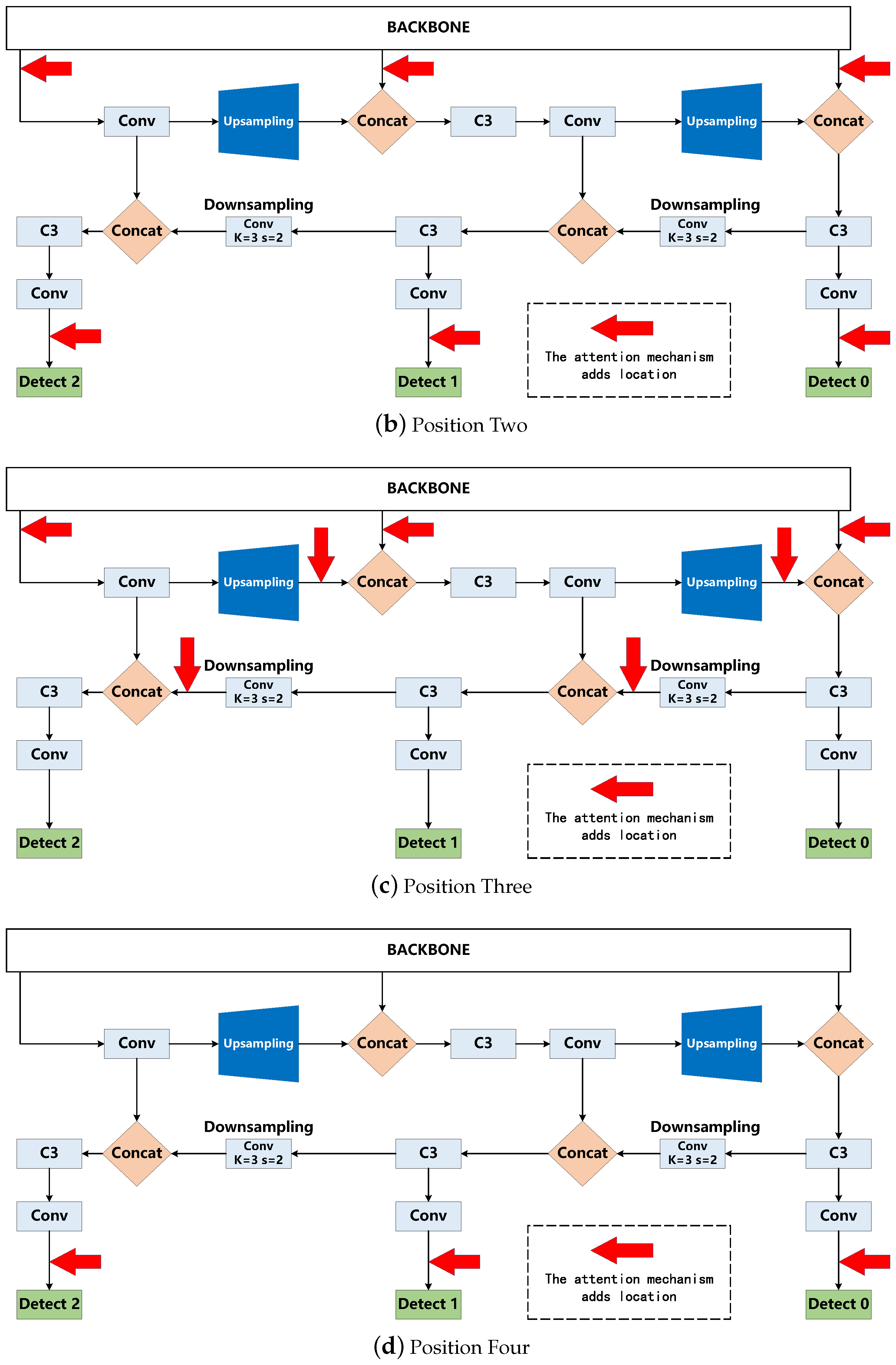
2.2. Attention Mechanism

The Attention Mechanism is a frequently used deep learning technique that improves the model’s capacity to focus on incoming data and to selectively highlight important information. By learning weights that only emphasize particular portions of the input throughout the aggregation process, it simulates human attention.

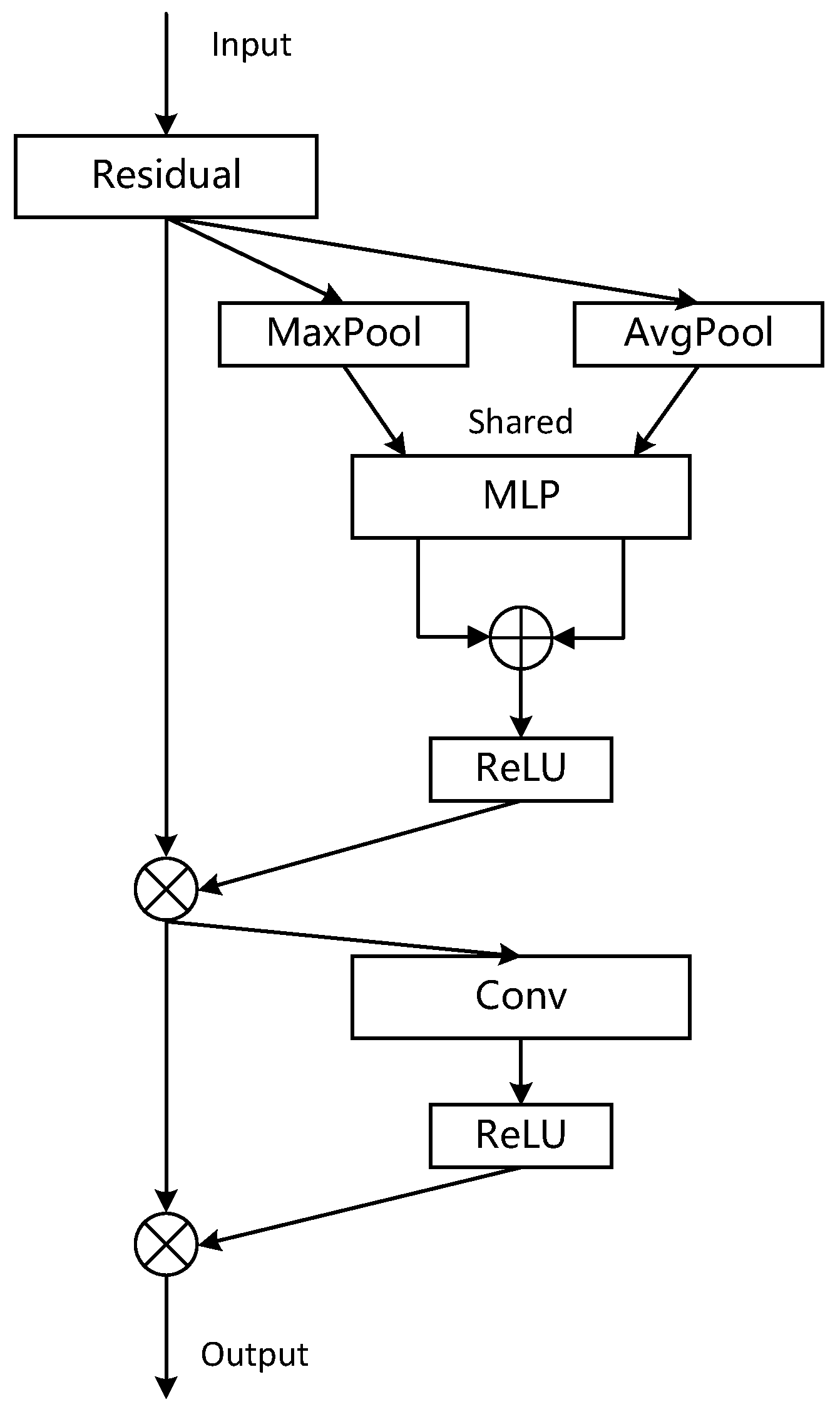
2.2.1. CBAM Attention Mechanism

The Channel Attention Module and the Spatial Attention Module are the two sub-modules that make up the CBAM (Convolutional Block Attention Module) attention mechanism [21]. To capture various degrees of feature representation, these sub-modules carry out attentional operations on several dimensions, namely the channel dimension and the spatial dimension, respectively.

The purpose of the Channel Attention Module is to record the relationships between the feature maps in the channel dimension. This is accomplished by using fully connected layers and global average pooling to learn channel weights, allowing the module to selectively enhance or suppress particular channels within the feature maps. This attention mechanism focuses the model’s attention on important channel information, leading to the extraction of representations that are more thorough and feature-rich.

The goal of the spatial attention module is to comprehend the spatial importance of the feature map. This is carried out by applying a number of operations to the feature graph, including maximum pooling, average pooling, convolution layers, and activation functions, to create a spatial attention graph. The features at different positions within the feature map are then given weights using this graph. As a result, the model may analyze characteristics at many locations while concentrating on important spatial information. Figure 6 provides a diagram of the procedure.

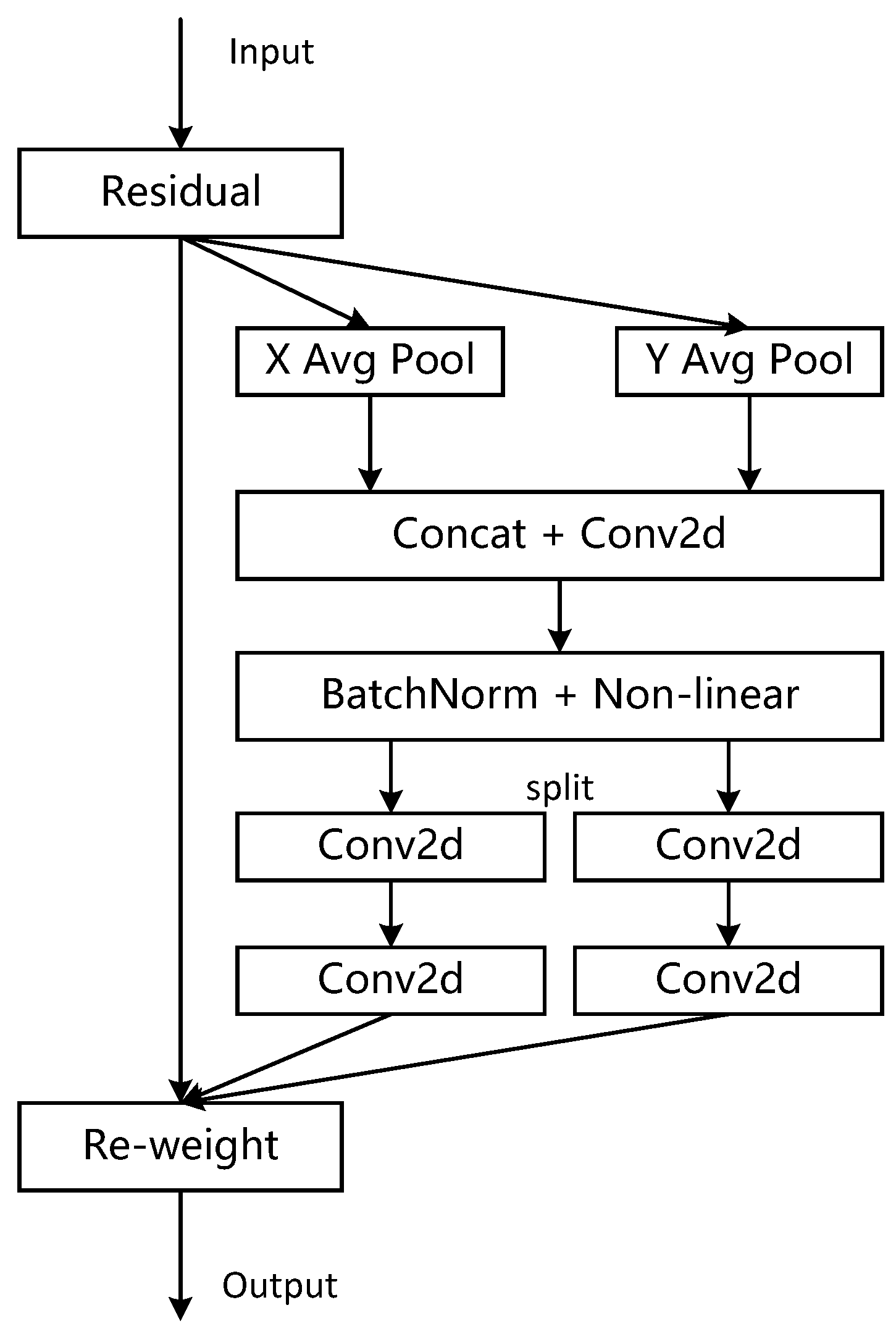
2.2.2. CA Attention Mechanisms

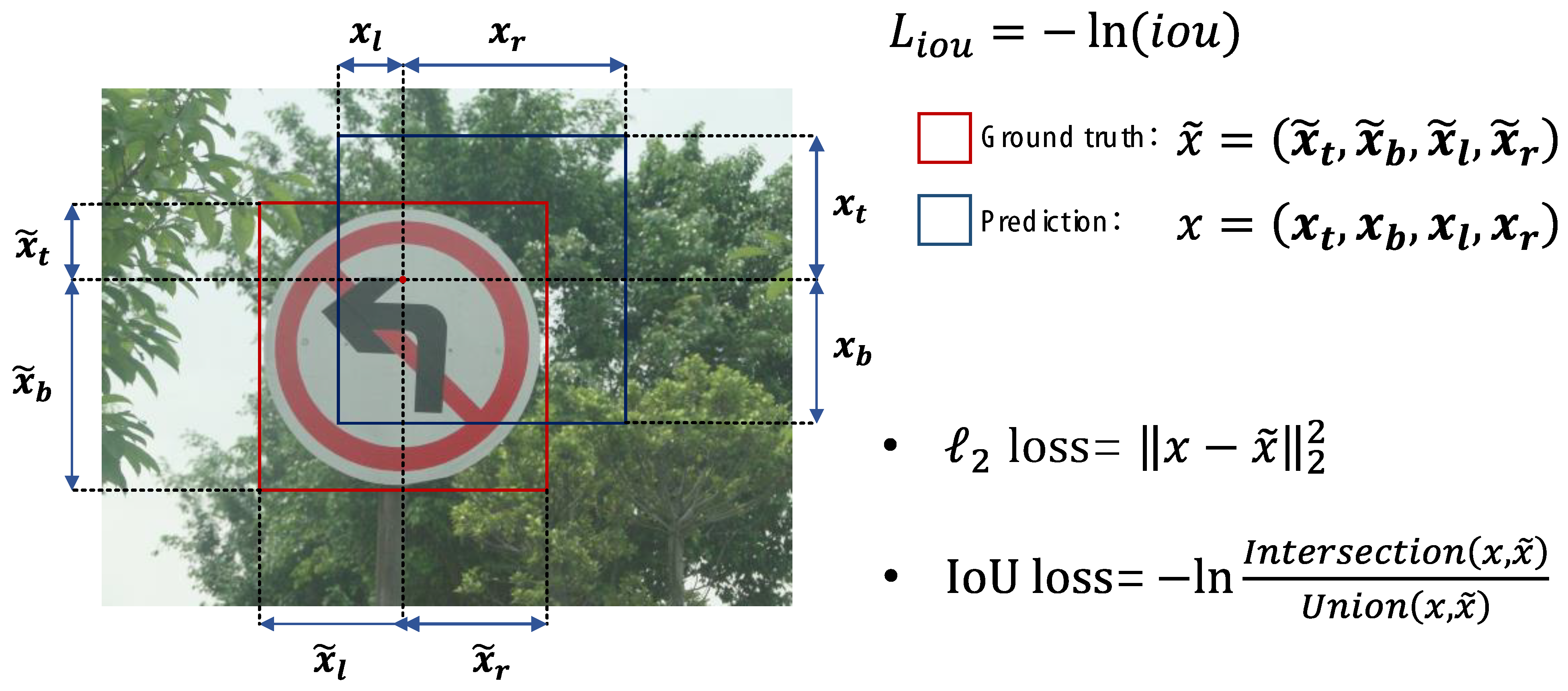
The feature map’s channels can be selectively enhanced or suppressed using the coordinate attention mechanism (CA). It makes it easier to extract richer and more important characteristics by learning channel weights [22]. In order to allow the model to prioritize important channel information during feature processing, CA primarily operates on the channel dimension of the feature map. For a visual illustration, see Figure 7.

2.3. IoU Loss

In many object detection tasks, the Intersection over Union (IoU) loss function is used, as shown in Figure 8 below [23]. The overlap between the anticipated bounding box and the actual labeling of the model output is measured by this loss function. The anticipated bounding box and the ground truth box’s common area is indicated by the intersection, while their combined area is shown by the union. By minimizing the IoU loss function during training, the model modifies the location and dimensions of the predicted bounding box with the goal of getting it to resemble the ground truth box as much as possible. The model may better capture the shape and location of the item by optimizing the IoU loss function, which raises the object detection accuracy.

2.3.1. EIoU Loss Function

The non-negativity, symmetry, triangle inequality, and scale insensitivity of the IoU loss function are all positive qualities. The loss value is 0 because it is unable to accurately gauge the distance between two boxes that do not intersect. A disadvantage of the IoU loss function is its delayed convergence.

The GIoU loss function is proposed as an improvement over the IoU loss function, which suffers from the limitation of always yielding a value of 0 when there is no intersection between two boxes [24]. Let A and B represent any two boxes and C represent the smallest box that encloses both A and B. The IoU is calculated as $|A\cap B|/|A\cup B|$. The GIoU loss function becomes valid when $|A\cap B|=0$. In such cases, the GIoU loss aims to increase the area of the bounding box to ensure overlap with the object box, contrary to the intuition of reducing the spatial location difference. When $|A\cap B|>0$, the area of $|C-A\cup B|$ is always a decimal or zero (this term is zero when A contains B, and vice versa). Consequently, the GIoU loss degenerates to the IoU loss in this scenario. As a result, the convergence rate of the GIoU loss remains slow.

$$L_{GIoU}=1-IoU+\frac{|C-(A\cup B\left)\right|}{\left|C\right|}$$

(4)

The CIoU loss function takes into account three crucial geometric elements: overlap area, center distance, and aspect ratio [25]. In this context, B represents the prediction frame, $B^{gt}$ denotes the object frame, and b and $b^{gt}$ represent the centroids of B and $B^{gt}$, respectively. The Euclidean distance between b and $b^{gt}$ is denoted as $\rho (·)=\parallel b-b_{gt}{\parallel }^2$. Additionally, c represents the diagonal of the smallest box that covers both boxes. The aspect ratio difference is measured by $v=\frac{4}{{\pi }^2}{(arctan\frac{w^{gt}}{h^{gt}}-arctan\frac{w}{h})}^2$, and $\alpha$ is computed as $\alpha$ = $\frac{v}{(1-IoU)+v}$.

The CIOU loss function is defined as follows:

$$L_{CIoU}=1-IoU+\frac{{\rho }^2(\mathbf{b},{\mathbf{b}}^{gt})}{c^2}+av$$

(5)

The EIoU (Efficient IoU) introduces improvements to the CIoU (Complete IoU) loss by addressing the aspect ratio inconsistency issue. It replaces the aspect ratio-related component of the CIoU loss with separate consistency losses for length and width. This modification results in the EIoU loss, which provides a more reasonable and accurate representation [26]. The definitions of the EIoU loss are as follows:

$$L_{EIoU}=L_{IoU}+L_{dis}+L_{asp}$$

(6)

$$\begin{array}{c}\hfill L_{EIoU}=1-IoU+\frac{{\rho }^2(\mathbf{b},{\mathbf{b}}^{gt})}{{\left(w^c\right)}^2+{\left(h^c\right)}^2}+\frac{{\rho }^2(w,w^{gt})}{{\left(w^c\right)}^2}+\frac{{\rho }^2(h,h^{gt})}{{\left(h^c\right)}^2}\end{array}$$

(7)

The loss function is divided into three parts: IOU loss $L_{IoU}$, distance loss $L_{dis}$, and direction loss $L_{asp}$. In this context, hw and hc represent the width and height of the minimum enclosing frame that covers the two boxes. Additionally, the EIOU loss is introduced to directly minimize the disparity between the object and anchor boxes’ width and height. This approach leads to faster convergence and improved localization.

2.3.2. SIoU Loss Function

The SIoU (SCYLLA-IoU) loss function incorporates traditional metrics such as distance, shape, and IoU to calculate the penalty for mismatches between the true value in the image and the model’s bounding box [27]. This addition significantly improves the training process by causing the prediction frame to converge quickly towards the nearest axis, allowing subsequent methods to rely on only one coordinate (X or Y) for regression. In essence, the introduction of angular penalty effectively reduces the overall degrees of freedom. The SIoU loss function comprises four cost functions: angle, distance, shape, and IoU. The angular cost function allows the model to make predictions in the X and Y axes first, and during convergence, attempts are made to minimize the value of $\alpha$ in $tan\alpha =\frac{Y}{X}$; the value of $\beta$ in $tan\beta =\frac{X}{Y}$ is minimized when $\alpha \le \frac{\pi }{4}$. The distance cost function is defined taking into account the angular cost defined above. When $\alpha \to 0$, the contribution of the distance cost is greatly reduced. Conversely, when $\alpha \to \frac{\pi }{4}$, the contribution of the distance cost is greater. The shape cost function is defined as

$$\Omega =\sum _{t=w,h}{(1-e^{-{\omega }_t})}^{\theta }$$

(8)

$${\omega }_w=\frac{|w-w^{gt}|}{max(w,w^{gt})},{\omega }_h=\frac{|h-h^{gt}|}{max(h,h^{gt})}$$

(9)

and the value of $\theta$ defines the shape cost, and its value is unique for each data set. $\theta$ controls the attention value required for the shape cost. If $\theta =1$, this will immediately optimize the shape and thus affect the free motion of the shape.

2.3.3. Wise IoU Loss Function

A problem of including low-quality data in the training dataset is that geometric measurements, such as distance and aspect ratio, might amplify the penalty applied to such samples, causing the model’s generalization performance to degrade. To solve this problem, an efficient loss function should reduce the penalty imposed by geometric metrics in cases when the anchor frame and the object frame strongly overlap. The model can acquire improved generalization skills by minimizing interference during training. A two-layer distance attention mechanism loss function based on the distance metric is introduced in this context by WIoU [28]. The dynamic non-monotonic focusing mechanism uses “outliers” as an alternative to IoU for quality assessment of anchor frames and provides a judicious gradient gain assignment strategy. This strategy reduces the competitiveness of high-quality anchor frames while reducing the harmful gradients generated by low-quality examples. This allows the WIoU to focus on anchor frames of average quality, improving the detection accuracy of the detector.

• ${\mathcal{R}}_{WIoU}\in \left[1,e\right)$; this will significantly amplify the ${\mathcal{L}}_{IoU}$ of the common mass anchor frame.
• ${\mathcal{L}}_{IoU}\in [0,1]$; this will significantly reduce the ${\mathcal{R}}_{WIoU}$ of high quality anchor frames and significantly reduce their focus on the center distance when the anchor frame is well overlapped with the object frame.

  $${\mathcal{L}}_{WIoUv1}={\mathcal{R}}_{WIoU}{\mathcal{L}}_{IoU}$$

  (10)

  $${\mathcal{R}}_{WIoU}=exp\left(\frac{{(x-x_{gt})}^2-{(y-y_{gt})}^2}{{(W_g^2-H_g^2)}^{*}}\right)$$

  (11)

In the above equation, $W_g$, $H_g$ are the length and width of the minimum outer bounding box of the prediction and real boxes. In order to prevent ${\mathcal{R}}_{WIoU}$ from generating gradients that impede convergence, $W_g$, $H_g$ are separated from the computational graph (the superscript * indicates this operation). Because it effectively eliminates the factors that hinder convergence, no new variables are introduced, such as the horizontal to vertical ratio, so the convergence efficiency of the model is improved.

3. Experimental Design

3.1. Experimental Dataset

Six wide-angle DSLR cameras with large pixel counts were used to create the TT100K traffic signs dataset [29], and various lighting and weather conditions were present at each shooting location. The dataset’s final size is 2048 × 2048, with the original image’s resolution being 8192 × 2048. The panorama was then divided into four pieces. There are more thorough categories of traffic signs in the TT100K dataset, which has 221 distinct categories overall and 128 tagged categories. This study randomly chooses 9050 photos with traffic signs from the TT100K dataset and reclassifies the categories because the number of categories in the dataset is seriously unequal. This study uses the CCTSDB dataset categorization standard to divide the dataset into three categories: required directional signs, prohibitory signs, and warning signs.

Table 1. 3L-TT100K dataset.

Classification	Quantity (pcs)
prohibitory	16,745
mandatory	4539
warning	1241

lists the numbers for each category under the designation 3L-TT100K. The 3L-TT100K with dimensions 2048 × 2048 is used as a model to accelerate model training and verify the model’s capacity to detect the target. The size of the 3L-TT100K dataset is shrunk to 640 × 640 from 2048 × 2048.

3.2. Evaluation Metrics

For assessing the consistency of test outcomes, the model assessment metrics utilized in this article use fixed IoU and confidence levels. The determination of precision and recall for the prediction outcomes allows for the measurement of the model’s object detection and object categorization capabilities. Additionally, by varying the confidence thresholds, precision–recall curves (P-R curves) can be created, providing a visual depiction of the model’s detection efficiency. Based on the true labels, the detection results are divided into four groups when the precision and recall metrics are computed: true positive ($TP$), true negative ($TN$), false positive ($FP$), and false negative ($FN$).

By evaluating the ratio of correctly predicted samples to all predicted samples in the detection results, precision is a statistic that assesses a model’s capacity to categorize an object. It is calculated as follows to indicate the ratio of successfully detected samples to all detected samples:

$$Precision=\frac{TP}{TP+FP}$$

(12)

Recall is a metric that gauges how well the model can identify the object. It is derived by dividing the number of real samples overall in the detection results by the proportion of samples that were correctly predicted. In other words, it symbolizes the proportion of successfully recognized samples to all true samples, offering information on the model’s detection abilities. It is calculated as follows:

$$Recall=\frac{TP}{TP+FN}$$

(13)

Recall is a metric that gauges how well the model can identify the object. It is derived by dividing the number of real samples overall in the detection results by the proportion of samples that were correctly predicted. In other words, it symbolizes the proportion of successfully recognized samples to all true samples, offering information on the model’s detection abilities. It is calculated as follows:

The average precision ($AP$) value derived by averaging the precision values along the precision–recall ($PR$) curve is represented by this term. It is computed by integrating the PR curve’s area under the curve.

$$AP={\int }_0^{1}p\left(r\right)dr$$

(14)

An essential evaluation statistic for object detection systems is the mean average precision (mAP). It provides a thorough evaluation of the model’s performance and is calculated as the average of the average precision ($AP$) values. To evaluate object detection algorithms, the speed and accuracy (mAP) metrics are frequently used, providing a fair knowledge of their capabilities. A more advanced object detection model for the particular dataset under consideration is indicated by a higher mAP value.

Furthermore, the quantity of sent frames per second (FPS) is used to gauge how quickly the algorithm detects motion. This statistic is a crucial gauge of how well the algorithm works in real-time detection.

4. Analysis of Experimental Results

4.1. Experimental Environment

The experiment was carried out in a Linux environment using the Ubuntu 20.04 operating system. The experimental device has an NVIDIA RTX3090 GPU with 24 GB of video RAM, Pytorch 1.11.0, Python 3.8, and CUDA 11.3 loaded to assist the experiment.

4.2. Experimental Setup

The network structure of both YOLOv5s and YOLOv5l models are shown in Figure 1, and the resultant frameworks of the two models are the same, with the YOLOv5l model having a parameter count that is about seven times larger than that of YOLOv5s by controlling the number of C3 modules. When the algorithm is trained, the parameters are tuned using both manual and genetic algorithms to prove that the algorithm in this paper is the optimal model. In the manual tuning experiment, the parameter optimiser, batch size, and learning rate (lr) were tuned. optimizerSGD, Adam, and AdamW were tuned in the middle of the three; the batch size was tuned between 32 and 64; and lr was tuned between 0.01 and 0.001, respectively. In the genetic algorithm (GA) evolutionary iteration of lr, a mutation technique with a probability of 80% and a variance of 004 was used to generate new offspring based on the best parent in the previous generations.The YOLOv5-EfficientViT algorithm migrated the weights of the EfficientViT network of ImageNet, and the model was trained for a total of 500 rounds. The results of parameter tuning are shown in

Table 2. Algorithm tuning test table.

Optimizer	Batch-Size	Learning Rate	mAp@0.5%
SGD	32	0.01	94.0%
SGD	64	0.01	93.9%
SGD	32	0.001	89.1%
Adam	32	0.01	84.1%
Adam	64	0.01	80.8%
Adam	32	0.001	92.5%
AdamW	32	0.01	93.2%
AdamW	64	0.01	92.9%
AdamW	32	0.001	92.0%
GA(SGD)	32	0.0136	94.1%

; different optimizers have a greater impact on the model, and the optimal optimizer is SGD. The batch size also has a certain impact on the model, and the smaller the batch-size, the better the results. The size of the learning rate affects the convergence speed of the model, and the optimal learning rate corresponding to different optimizers is also the optimal learning rate for different optimizers.

4.3. Algorithm Detection Performance Comparison Analysis

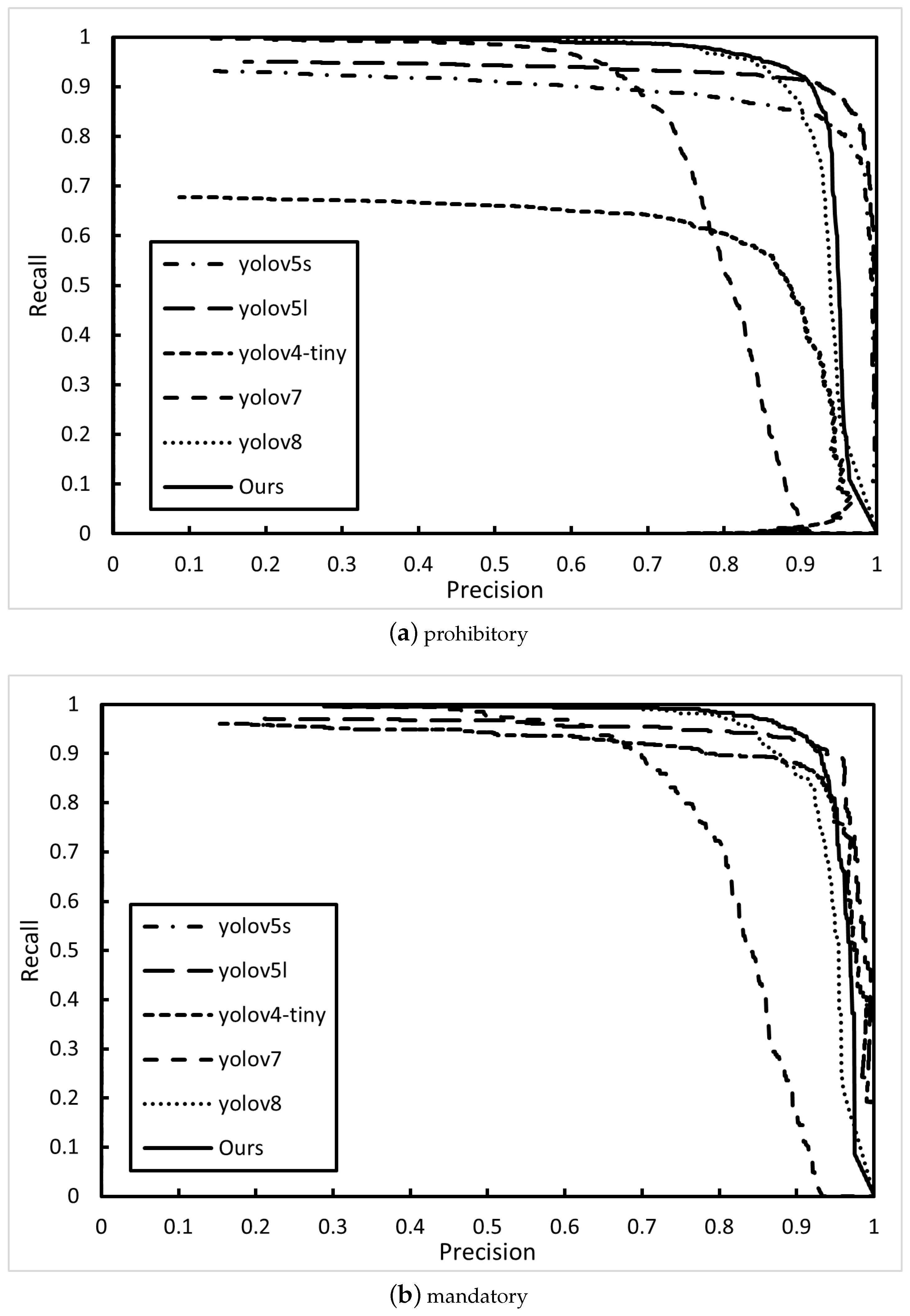
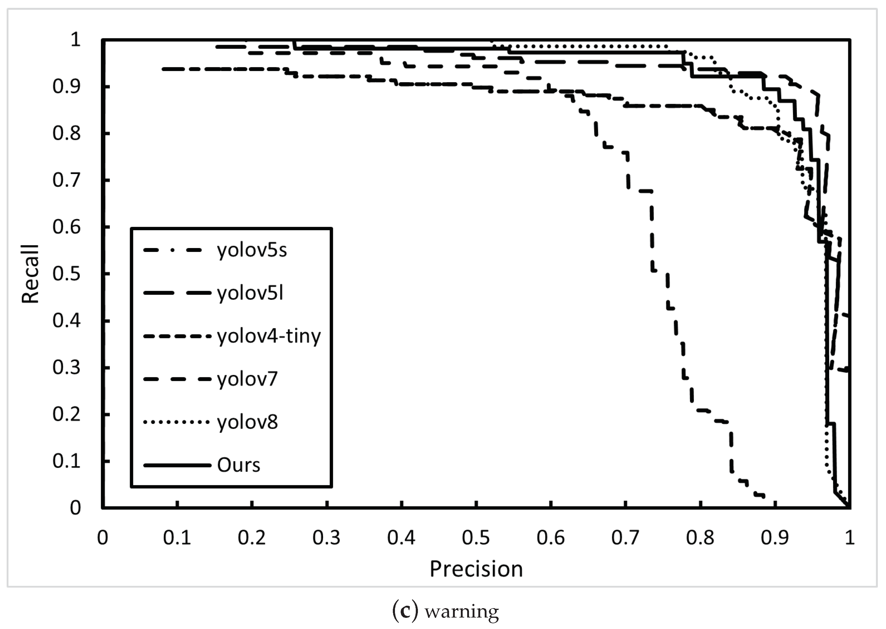
4.3.1. Algorithm P-R Curve Comparison

To assess the detection performance of the algorithm, we conducted tests comparing YOLOv5-EfficientViT with YOLOv5(s), YOLOv5(l), YOLOv4-tiny, YOLOv7, and YOLOv8. These three categories were used to validate the five methods on the TT100K dataset, and

Table 3. Comparison table of P-R curves of algorithms.

Algorithm	Parameters	Prohibitory	Mandatory	Warning
YOLOv5(s)	P	95.87%	94.64%	93.00%
	R	80.08%	79.85%	73.23%
YOLOv5(l)	P	96.05%	96.25%	95.54%
	R	86.43%	87.01%	84.25%
YOLOv4-tiny	P	76.72%	75.27%	81.73%
	R	61.52%	65.35%	66.93%
YOLOv7	P	89.4%	91.7%	67.6%
	R	68.7%	67.6%	73.3%
YOLOv8	P	92.8%	92.9%	87.4%
	R	84.9%	84.9%	89.4%
YOLOv5-EfficientViT(Ours)	P	93.50%	93.70%	88.10%
	R	88.3%	90.6%	90.4%

shows the experimental outcomes. Additionally, we produced P-R curves to graphically display the algorithm’s effectiveness on this dataset. In Figure 9, below, these curves are shown.

The self-attention mechanism from the transformer is used by the YOLOv5-EfficientViT method to improve the analysis and processing of global characteristics in images. This algorithm outperforms other widely used detection techniques in terms of recall rates for the detection of the three item classes indicated in Table 3. In addition, it achieves significant accuracy gains over YOLOv4-tiny, YOLOv7, and YOLOv8.

The P-R curve in Figure 9a indicates that the current approach outperforms two widely used object identification algorithms, YOLOv4-tiny, YOLOv7, and YOLOv8, in terms of detecting prohibitory category objects. This conclusion is supported by the rest of Figure 9. Furthermore, the P-R curves shown in Figure 9b,c unmistakably show that the current approach outperforms the YOLOv7 object detection algorithm in terms of recognizing mandatory class and warning items. Notably, the 3L-TT100K dataset consistently performs better than the other five object detection algorithms for all three classes of objects when the precision is 0.9.

4.3.2. Comparative Analysis of Algorithm in Real-Time

A comparison and study of frames per second (FPS) between the algorithm described in this research and the YOLOv5(s), YOLOv5(l), YOLOv4-tiny, YOLOv7, and YOLOv8 algorithms are completed to verify the real-time performance of the approach.

Table 4. Algorithm inference speed comparison.

Algorithm	FPS (frame/s)
YOLOv5(s)	44.47
YOLOv5(l)	39.30
YOLOv4-tiny	122.06
YOLOv7	64.52
YOLOv8	65.70
YOLOv5-EfficientViT(Ours)	62.50

presents the outcomes. The fastest of these algorithms, YOLOv4-tiny, processes 122.06 images per second, while YOLOv5(l) processes 39.30 images per second. The processing rate of the algorithm used in this study is 62.50 images per second, which is slightly slower than the YOLOv7 and YOLOv8 object detection algorithms. The approach presented in this study accelerates feature map extraction and provides noticeably faster image processing speeds than both the YOLOv5(s) and YOLOv5(l) algorithms by substituting the YOLOv5 backbone with the EfficientViT network. The technique described in this research ensures that the required image processing speed for real-time detection while maintaining a balance between detection accuracy and real-time performance when compared to several standard object detection algorithms. Considering the lack of such a high-performance hardware equipment configuration in the test in the application scenario, the algorithm in this paper was verified in the test on the 2080 ti, which can process 57.80 pictures per second and can meet the requirements of real-time detection, with good applicability.

4.3.3. Comparative Analysis of Algorithmic Ablation Experiments

A number of comparative ablation experiments were carried out in order to better understand the internal network structure of the YOLOv5-EfficientViT algorithm and gauge the effect of modules with various architectures on its detection performance. The backbone network replacement, the insertion of attention mechanisms at various locations, and the replacement of the IoU loss function were the three main focuses of the ablation experiment design. Four network architectures were used for the backbone replacement: Mobilenetv3, EfficientFormerv2, Efficient Model (EMO), and EfficientViT. We investigated the impact of backbone model size on detection performance using the Mobilenetv3 network, a lightweight network that has gained popularity recently, and the latter three models, which are Vision Transformer models with improved detection performance.

The results of the ablation experiment are shown in

Table 5. Comparison of ablation experiment results.

Number	Backbone	Attention Mechanisms	IoU Loss	mAP@0.5%	FPS (frame/s)
1	Mobilenetv3	-	-	83.2 %	85.47
2	EfficientFormerv2(s1)	-	-	92.7 %	32.26
3	EfficientFormerv2(l)	-	-	94.4%	29.59
4	EMO(1M)	-	-	93.5 %	60.61
5	EMO(6M)	-	-	93.7 %	54.05
6	EfficientViT(b1)	-	-	93.7 %	62.89
7	EfficientViT(b2)	-	-	93.8 %	53.19
8	EfficientViT(b1)	CA(a)	-	92.5 %	56.50
9	EfficientViT(b1)	CA(b)	-	93.4 %	56.50
10	EfficientViT(b1)	CA(c)	-	92.5 %	55.56
11	EfficientViT(b1)	CA(d)	-	92 %	52.36
12	EfficientViT(b1)	CBAM(a)	-	93.7 %	54.64
13	EfficientViT(b1)	CBAM(b)	-	93%	57.14
14	EfficientViT(b1)	CBAM(c)	-	93.4 %	53.48
15	EfficientViT(b1)	CBAM(d)	-	93.8%	62.11
16	EfficientViT(b1)	-	SIoU	90.8 %	71.94
17	EfficientViT(b1)	-	EIOU	91.2%	67.57
18	EfficientViT(b1)	-	Wise IoU	93.9%	63.29
19	EfficientViT(Ours)	CBAM(d)	Wise IoU	94.1%	62.50

, which contrasts the backbone replacements for the YOLOv5 model with the Mobilenetv3 network (which achieved the fastest processing speed of 85.47 FPS for images) and the EfficientFormerv2 (l) network (which produced the best detection performance with a mAP of 94.4%). The YOLOv5-EfficientViT backbone was created by replacing the YOLOv5 backbone with the EfficientViT (b1) network after taking into account both detection accuracy (mAP) and speed (FPS) measures in comparison with YOLOv5. (From here on, EfficientViT will always refer to the EfficientViT (b1) model).

An attention mechanism is introduced to improve attention to the input and selectively focus on important information during feature extraction. As shown in Figure 10a–d, we chose the CA attention network and the CBAM attention network for this study and included them in the model. As shown in Table 5, when using EfficientViT as the backbone and positioning the Tim CBAM attention network at position Figure 10d, the algorithm achieves the best object detection results in terms of mAP and FPS. Notably, compared to adding the CA attention network at the same site, adding the CBAM attention network in Figure 10d results in a 1.8-point gain in object detection accuracy and a 9.75 images per second increase in detection speed. Additionally, utilizing YOLOv5-EfficientViT without the attention mechanism results in a 0.1% improvement in detection accuracy.

In order to improve the YOLOv5-EfficientViT algorithm, this work introduces four loss functions, namely EIoU, SIoU, and WIoU. Table 5 makes it very evident that using the WIoU loss function increases the algorithm’s detection accuracy in comparison to YOLOv5-EfficientViT by 0.2 percentage points. Additionally, the technique improves speed by 0.4 images per second. Incorporating the CBAM attention mechanism, the WIoU loss function, and the replacement of the YOLOv5 backbone with EfficientViT at position (d) in Figure 10 make up the entire algorithm structure of this study. The addition of the WIoU loss function improves the accuracy of traffic signage by 0.2 percentage points and improves the inference speed by 1 FPS. Table 5 displays the experimental findings. The algorithm used in this study improves the detection accuracy in terms of mAP by 4.76 percentage points in comparison to the YOLOv5s model and accelerates detection by 18.03 photos per second.

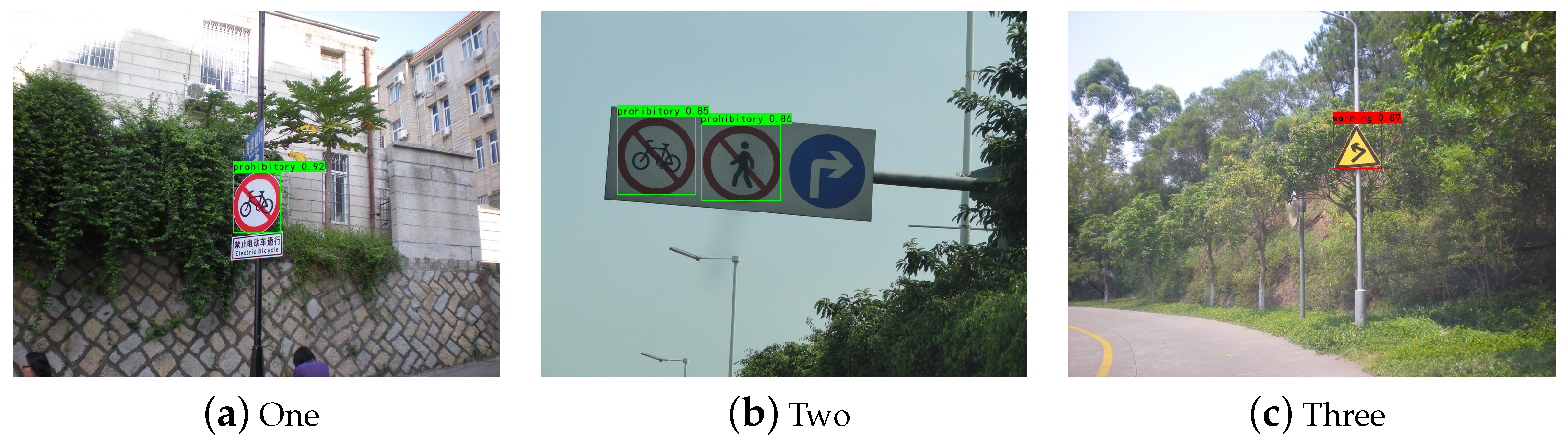
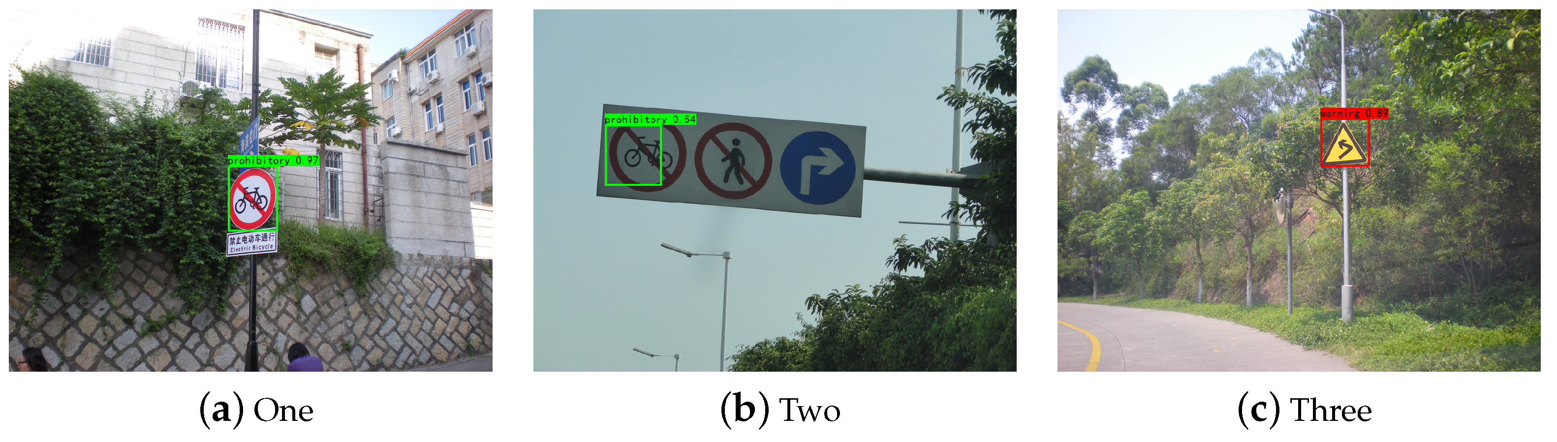
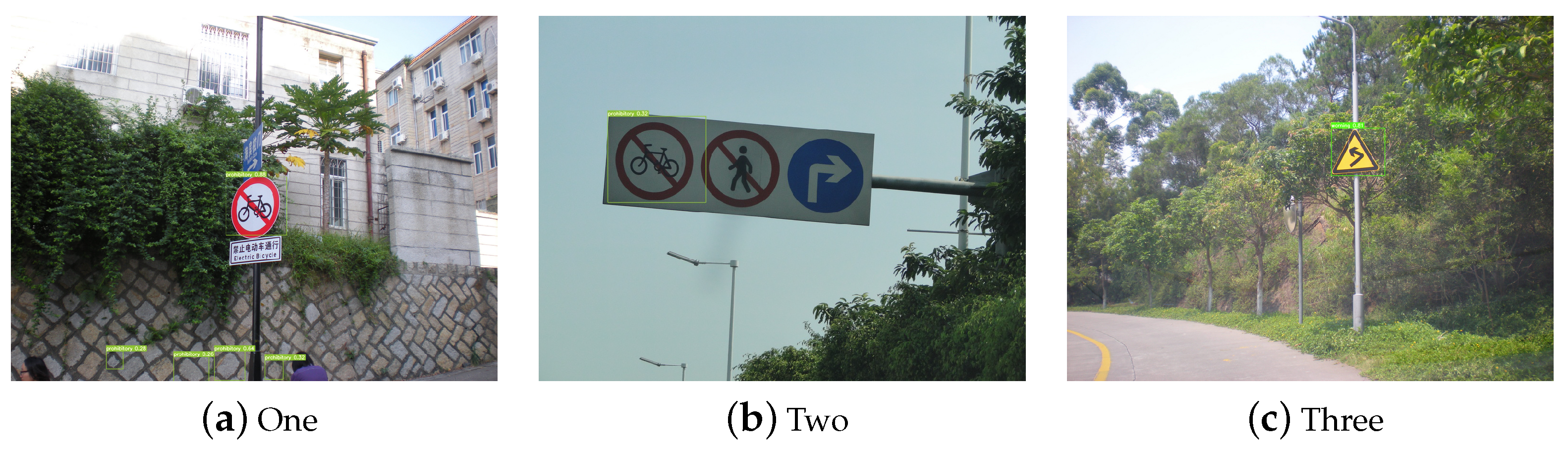
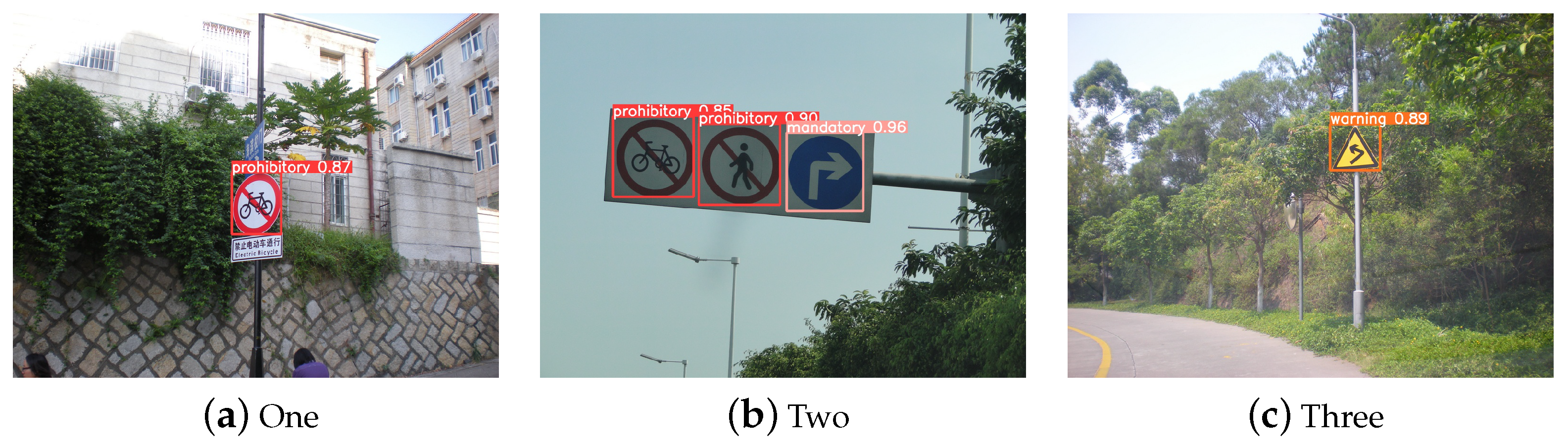
4.3.4. Comparative Analysis of Experimental Results of Algorithm Detection Accuracy

Using the 3L-TT100K dataset, the current algorithm is evaluated against the YOLOv5(s), YOLOv5(l), YOLOv4-tiny, YOLOv, and YOLOv8 algorithms. The mean average precision (mAP) for each algorithm is calculated after a thorough analysis of the average precision (AP) of each algorithm for several categories, as shown in

Table 6. Comparison of algorithm detection accuracy results.

Algorithm	Prohibitory AP	Mandatory AP	Warnin AP	mAP
YOLOv5(s)	89.37%	91.33%	87.32%	89.34%
YOLOv5(l)	93.11%	94.51%	94.69%	94.1%
YOLOv4-tiny	60.29%	60.01%	67.76%	62.69%
YOLOv7	78.8%	81.6%	72.2%	77.6%
YOLOv8	91.7%	92.6%	92.5%	92.3%
ETSR-YOLO	-	-	-	88.3%
TRD-YOLO	-	-	-	86.3%
CR-YOLOv8	-	-	-	86.9%
YOLOv5-EfficientViT(Ours)	93.7%	95.4%	93.2%	94.1%

below. For all three types of tags in the 3L-TT100K dataset, the algorithm reported in this paper surpasses YOLOv5(s), YOLOv4-tiny, YOLOv7, and YOLOv8 algorithms in terms of detection accuracy. Compared with the method in this study, YOLOv5(l) has a higher detection accuracy, and according to the comprehensive analysis of Table 4 and Table 6, the algorithm in this paper has the advantages of high detection accuracy and speed. In order to prove that the detection performance of this paper’s algorithm is better than the existing state-of-the-art traffic sign detection algorithms, the algorithm in this paper is compared with ETSR-YOLO [30], TRD-YOLO [31], and CR-YOLOv8 [32], and the accuracy of traffic sign detection is better than the three traffic sign target detection algorithms mentioned above.

4.4. Algorithm Detection Performance Comparison Analysis

This research assesses the algorithms by contrasting them with YOLOv5(s), YOLOv5(l), YOLOv4-tiny, YOLOv7, and YOLOv8 on the validation set of the 3L-TT100K dataset. This comparison helps to promote a more natural comparison of the detection performance among methods. Only the prediction frames with a confidence level higher than 0.5 are kept for the validation testing.

In the figures below, Figure 11, Figure 12, Figure 13, Figure 14, Figure 15, Figure 16 and Figure 17, the validation findings are shown. The image under detection is shown in Figure 11, where Figure 11a shows how the backdrop and signage features are quite similar, interfering with the algorithm used to recognize the signs. The YOLOv7 algorithm’s detection result, shown in Figure 15a, wrongly classifies background information as signage. On the other hand, Figure 17a shows the detection outcome produced by the algorithm suggested in this study. This approach improves the extraction of object information in the feature layer by including the CBAM attention mechanism, considerably lowering the incidence of false detections by the detection algorithm.

The YOLOv5l algorithm fails to identify mandatory-type signs in Figure 12b, Figure 14b, and Figure 15b when attempting to recognize the signage seen in Figure 11b. The detection results of the YOLOv5l method, which successfully detects the mandatory class flag, are shown in Figure 13b. However, compared to the 0.76 attained by the algorithm suggested in this research, the confidence level of the algorithm’s detection is just 0.5. The algorithm presented in this research makes use of the self-attention mechanism in the EfficientViT backbone to extract information on the global feature layer order and content, enhancing detection precision and decreasing the number of missed detection cases. The detection effects of the YOLOv4-tiny algorithm and the YOLOv7 algorithm, respectively, are shown in Figure 14b and Figure 15b. The findings show unequivocally that both methods provide prediction frames that considerably differ from the detection item, leading to subpar detection performance. The technique suggested in this paper proposes the WIoU loss function, which modifies the weights of superior and inferior prediction frames to minimize the deviation value between the prediction frame and the detection object, in order to address the problem of severe frame deviation.

Figure 16 shows the detection effect of the YOLOv8 algorithm. From Figure 16a,b, it can be seen that the overall detection accuracy is worse than the model in this paper. The methods suggested in this paper provide higher detection performance compared to existing mainstream detection algorithms for the warning class signage, especially taking into account the limited training samples available, as shown in Figure 12c, Figure 13c, Figure 14c, Figure 15c, Figure 16c and Figure 17c.

The YOLOv5-EfficientViT algorithm proposed in this paper, which effectively addresses the limitations of conventional networks, such as missed detections and errors, by leveraging its strong feature extraction capabilities and precise object frame positioning, has been verified through a comparative analysis of the aforementioned six groups of detection models. The experimental findings show that the algorithm performs quite well in terms of accuracy and real-time performance when it comes to detecting traffic signs. It excels in real-time traffic sign detection and outperforms currently used techniques.

5. Conclusions

The identification of traffic signs is crucial for study in the areas of traffic asset exclusion, aided driving, and autonomous driving. In this research, we offer an accurate and fast traffic sign identification system based on the single-stage YOLOv5 algorithm and using EfficientViT as the foundation. We overcome the problem of the CSPDarkNet network’s failure to extract the global feature layer order and content information by relocating the self-attention mechanism from the transformer to object detection. The detection accuracy and real-time performance of traffic signage are both improved by this self-attention module. In order to improve the FPN stage’s ability to extract features, we also incorporate the CBAM attention method. In addition, the model’s convergence is sped up by using the WIoU loss function. Ablation experiments that contrast the impacts of the backbone network, attention mechanism, and loss function on the model serve to demonstrate the use of these modules.

On the 3L-TT100K dataset, our approach outperforms conventional mainstream techniques by achieving an mAP of 94.1% and a frame rate of 62.50 frames per second (FPS) for traffic sign detection. Our approach enhances the mAP by 4.76% when compared to the YOLOv5s algorithm on the same dataset. To balance the quantity of labels in the dataset and lessen the effect of label imbalances on accuracy, we plan to address the issue of label proportions during model training in future research.

References

1. Wang, Z.; Wang, J.; Li, Y.; Wang, S. Traffic sign recognition with lightweight two-stage model in complex scenes. IEEE Trans. Intell. Transp. Syst. 2020, 23, 1121–1131. [Google Scholar] [CrossRef]
2. Kukkala, V.K.; Tunnell, J.; Pasricha, S.; Bradley, T. Advanced driver-assistance systems: A path toward autonomous vehicles. IEEE Consum. Electron. Mag. 2018, 7, 18–25. [Google Scholar] [CrossRef]
3. Nandi, D.; Saif, A.S.; Prottoy, P.; Zubair, K.M.; Shubho, S.A. Traffic sign detection based on color segmentation of obscure image candidates: A comprehensive study. Int. J. Mod. Educ. Comput. Sci. 2018, 10, 35. [Google Scholar] [CrossRef]
4. Zaklouta, F.; Stanciulescu, B. Real-time traffic sign recognition in three stages. Robot. Auton. Syst. 2014, 62, 16–24. [Google Scholar] [CrossRef]
5. Vitabile, S.; Pollaccia, G.; Pilato, G.; Sorbello, F. Road signs recognition using a dynamic pixel aggregation technique in the HSV color space. In Proceedings of the Proceedings 11th International Conference on Image Analysis and Processing, Palermo, Italy, 26–28 September 2001; pp. 572–577. [Google Scholar]
6. Yakimov, P.; Fursov, V. Traffic signs detection and tracking using modified hough transform. In Proceedings of the 2015 12th International Joint Conference on e-Business and Telecommunications (ICETE), Colmar, France, 20–22 July 2015; Volume 5, pp. 22–28. [Google Scholar]
7. Balali, V.; Jahangiri, A.; Machiani, S.G. Multi-class US traffic signs 3D recognition and localization via image-based point cloud model using color candidate extraction and texture-based recognition. Adv. Eng. Inform. 2017, 32, 263–274. [Google Scholar] [CrossRef]
8. Zhang, J.; Xie, Z.; Sun, J.; Zou, X.; Wang, J. A cascaded R-CNN with multiscale attention and imbalanced samples for traffic sign detection. IEEE Access 2020, 8, 29742–29754. [Google Scholar] [CrossRef]
9. Gao, B.; Jiang, Z.; Zhang, J. Traffic Sign Detection based on SSD. In Proceedings of the 2019 4th International Conference on Automation, Control and Robotics Engineering, Shenzhen, China, 19–21 July 2019. [Google Scholar]
10. Ren, S.; He, K.; Girshick, R.; Sun, J. Faster r-cnn: Towards real-time object detection with region proposal networks. Adv. Neural Inf. Process. Syst. 2015, 28. [Google Scholar] [CrossRef] [PubMed]
11. Qian, R.; Liu, Q.; Yue, Y.; Coenen, F.; Zhang, B. Road surface traffic sign detection with hybrid region proposal and fast R-CNN. In Proceedings of the 2016 12th International Conference on Natural Computation, Fuzzy Systems and Knowledge Discovery (ICNC-FSKD), Changsha, China, 13–15 August 2016; pp. 555–559. [Google Scholar]
12. Zuo, Z.; Yu, K.; Zhou, Q.; Wang, X.; Li, T. Traffic signs detection based on faster r-cnn. In Proceedings of the 2017 IEEE 37th International Conference on Distributed Computing Systems Workshops (ICDCSW), Atlanta, GA, USA, 5–8 June 2017; pp. 286–288. [Google Scholar]
13. Liu, W.; Anguelov, D.; Erhan, D.; Szegedy, C.; Reed, S.; Fu, C.Y.; Berg, A.C. Ssd: Single shot multibox detector. In Proceedings of the Computer Vision–ECCV 2016: 14th European Conference, Amsterdam, The Netherlands, 11–14 October 2016; pp. 21–37. [Google Scholar]
14. Lin, T.Y.; Goyal, P.; Girshick, R.; He, K.; Dollár, P. Focal loss for dense object detection. In Proceedings of the IEEE International Conference on Computer Vision, Venice, Italy, 22–29 October 2017; pp. 2980–2988. [Google Scholar]
15. Redmon, J.; Farhadi, A. YOLO9000: Better, faster, stronger. In Proceedings of the IEEE Conference on Computer Vision and Pattern Recognition, Honolulu, HI, USA, 21–26 July 2017; pp. 7263–7271. [Google Scholar]
16. Redmon, J.; Farhadi, A. Yolov3: An incremental improvement. arXiv 2018, arXiv:1804.02767. [Google Scholar]
17. Bochkovskiy, A.; Wang, C.Y.; Liao, H.Y.M. Yolov4: Optimal speed and accuracy of object detection. arXiv 2020, arXiv:2004.10934. [Google Scholar]
18. Vaswani, A.; Shazeer, N.; Parmar, N.; Uszkoreit, J.; Jones, L.; Gomez, A.N.; Kaiser, Ł.; Polosukhin, I. Attention is all you need. arXiv 2017, arXiv:1706.03762. [Google Scholar]
19. Dosovitskiy, A.; Beyer, L.; Kolesnikov, A.; Weissenborn, D.; Zhai, X.; Unterthiner, T.; Dehghani, M.; Minderer, M.; Heigold, G.; Gelly, S.; et al. An image is worth 16x16 words: Transformers for image recognition at scale. arXiv 2020, arXiv:2010.11929. [Google Scholar]
20. Cai, H.; Gan, C.; Han, S. EfficientViT: Enhanced Linear Attention for High-Resolution Low-Computation Visual Recognition. arXiv 2022, arXiv:2205.14756. [Google Scholar]
21. Woo, S.; Park, J.; Lee, J.Y.; Kweon, I.S. Cbam: Convolutional block attention module. In Proceedings of the European Conference on Computer Vision (ECCV), Munich, Germany, 8–14 September 2018; pp. 3–19. [Google Scholar]
22. Hou, Q.; Zhou, D.; Feng, J. Coordinate attention for efficient mobile network design. In Proceedings of the IEEE/CVF Conference on Computer Vision and Pattern Recognition, Nashville, TN, USA, 20–25 June 2021; pp. 13713–13722. [Google Scholar]
23. Yu, J.; Jiang, Y.; Wang, Z.; Cao, Z.; Huang, T. Unitbox: An advanced object detection network. In Proceedings of the 24th ACM International Conference on Multimedia, Amsterdam, The Netherlands, 15–19 October 2016; pp. 516–520. [Google Scholar]
24. Rezatofighi, H.; Tsoi, N.; Gwak, J.; Sadeghian, A.; Reid, I.; Savarese, S. Generalized intersection over union: A metric and a loss for bounding box regression. In Proceedings of the IEEE/CVF Conference on Computer Vision and Pattern Recognition, Long Beach, CA, USA, 15–20 June 2019; pp. 658–666. [Google Scholar]
25. Zheng, Z.; Wang, P.; Liu, W.; Li, J.; Ye, R.; Ren, D. Distance-IoU loss: Faster and better learning for bounding box regression. In Proceedings of the AAAI Conference on Artificial Intelligence, New York, NY, USA, 7–12 February 2020; Volume 34, pp. 12993–13000. [Google Scholar]
26. Zhang, Y.F.; Ren, W.; Zhang, Z.; Jia, Z.; Wang, L.; Tan, T. Focal and efficient IOU loss for accurate bounding box regression. Neurocomputing 2022, 506, 146–157. [Google Scholar] [CrossRef]
27. Gevorgyan, Z. SIoU loss: More powerful learning for bounding box regression. arXiv 2022, arXiv:2205.12740. [Google Scholar]
28. Tong, Z.; Chen, Y.; Xu, Z.; Yu, R. Wise-IoU: Bounding Box Regression Loss with Dynamic Focusing Mechanism. arXiv 2023, arXiv:2301.10051. [Google Scholar]
29. Zhu, Z.; Liang, D.; Zhang, S.; Huang, X.; Li, B.; Hu, S. Traffic-sign detection and classification in the wild. In Proceedings of the IEEE Conference on Computer Vision and Pattern Recognition, Las Vegas, NV, USA, 27–30 June 2016; pp. 2110–2118. [Google Scholar]
30. Liu, H.; Zhou, K.; Zhang, Y.; Zhang, Y. ETSR-YOLO: An improved multi-scale traffic sign detection algorithm based on YOLOv5. PLoS ONE 2023, 18, e0295807. [Google Scholar] [CrossRef] [PubMed]
31. Chu, J.; Zhang, C.; Yan, M.; Zhang, H.; Ge, T. TRD-YOLO: A real-time, high-performance small traffic sign detection algorithm. Sensors 2023, 23, 3871. [Google Scholar] [CrossRef] [PubMed]
32. Zhang, L.J.; Fang, J.J.; Liu, Y.X.; Feng Le, H.; Rao, Z.Q.; Zhao, J.X. CR-YOLOv8: Multiscale object detection in traffic sign images. IEEE Access 2023, 12, 219–228. [Google Scholar] [CrossRef]
Figure 1. YOLOv5(s) object detection model structure.
Electronics 13 00880 g001
Figure 2. YOLOv5 -EfficientViT (Ours) object detection model structure.
Electronics 13 00880 g002
Figure 3. EfficientViT general structure.
Electronics 13 00880 g003
Figure 4. MBConv structure.
Electronics 13 00880 g004
Figure 5. EfficientViT module structure.
Electronics 13 00880 g005
Figure 6. CBAM attention mechanism.
Electronics 13 00880 g006
Figure 7. CA attention mechanism.
Electronics 13 00880 g007
Figure 8. IoU Loss.
Electronics 13 00880 g008
Figure 9. P-R curve comparison. (a) is the Prohibitory traffic sign P-R curve; (b) is the Mandatory traffic sign P-R curve; (c) is the Warning traffic sign P-R curve.
Electronics 13 00880 g009aElectronics 13 00880 g009b
Figure 10. Comparison of total communication delay for different penetration rates of CAV.
Electronics 13 00880 g010aElectronics 13 00880 g010b
Figure 11. Original picture(Object detection model input image).
Electronics 13 00880 g011
Figure 12. YOLOv5(s) object detection model output results.
Electronics 13 00880 g012
Figure 13. YOLOv5(l) object detection model output results.
Electronics 13 00880 g013
Figure 14. YOLOv4-tiny object detection model output results.
Electronics 13 00880 g014
Figure 15. YOLOv7 object detection model output results.
Electronics 13 00880 g015
Figure 16. YOLOv8 object detection model output results.
Electronics 13 00880 g016
Figure 17. YOLOv5-EfficienntViT (Ours) object detection model output results.
Electronics 13 00880 g017