Bridging the Cybersecurity Gap: A Comprehensive Analysis of Threats to Power Systems, Water Storage, and Gas Network Industrial Control and Automation Systems

Abstract

This research addresses the dearth of real-world data required for effective neural network model building, delving into the crucial field of industrial control and automation system (ICS) cybersecurity. Cyberattacks against ICS are first identified and then generated in an effort to raise awareness of vulnerabilities and improve security. This research aims to fill a need in the existing literature by examining the effectiveness of a novel approach to ICS cybersecurity that draws on data from real industrial settings. Real-world data from a variety of commercial sectors is used in this study to produce a complete dataset. These sectors include power systems, freshwater tanks, and gas pipelines, which together provide a wide range of commercial scenarios where anomaly detection and attack classification approaches are critical. The generated data are shown to considerably improve the models’ precision. An amazing 71% accuracy rate is achieved in power system models, and incorporating generated data reliably increases network speed. Using generated data, the machine learning system achieves an impressive 99% accuracy in a number of trials. In addition, the system shows about 90% accuracy in most studies when applied to the setting of gas pipelines. In conclusion, this article stresses the need to improve cybersecurity in vital industrial sectors by addressing the dearth of real-world ICS data. To better understand and defend against cyberattacks on industrial machinery and automation systems, it demonstrates how generative data can improve the precision and dependability of neural network models.

1. Introduction

Modern business processes use industrial control systems (ICSs) to manage and regulate industrial processes and machinery, and a variety of businesses and sectors rely on ICSs. Keeping complicated machinery and processes running smoothly, safely, and reliably is the goal of these monitoring and control systems, which are vulnerable to cybersecurity risks due to their digitization and interconnection. ICS engineers manage computer networks, mechanical and electrical equipment, and human and automated tasks in an ICS. In the present scenario, production, power utilities, water storage systems, gas pipelines, and various other industries can use ICSs for a more robust and innovative environment [1]. ICS attacks can interrupt activities, disable machinery, undermine industrial procedures, and even endanger people. To protect these networks from attacks via the internet, they must be identified and fixed. Vulnerability studies and implementation must identify and generate commercial management system assaults. Analyzing ICSs involves methods of communication and ways to be attacked. Security experts and system administrators can improve critical network safety by analyzing risks and locations for attacks. Commercial control mechanisms are complex, making vulnerability and attack channel identification difficult. In contrast to standard IT systems, ICS settings have long lifespans with outdated equipment and older applications that may lack security patches. It is also important to comprehend ICS networks’ specialized methods of communication and technologies [2].

Multi-faceted testing is needed to find ICS flaws and weaknesses. This method combines risk assessments, hacking tests, and ICS architecture analysis. Vulnerability evaluations detect software, network structure, and system setting weaknesses. Security experts can assess security and detect attack points using machine learning techniques and human evaluation. Ethical hacking—penetration testing—simulates practical problems and attacks [3,4]. This entails exploiting flaws to access important systems. Penetration analysis evaluates safety measures, ICS-responsive features, and possibilities for growth [5,6]. Threat sources, intelligence, and internal evaluations are needed to stay abreast of new corporate control system assault methods [7,8]. Threat analysis informs about ICS-specific risks, viruses, and attack operations. Industries can prevent cyberattacks and strengthen security by tracking threats and comprehending their methods. Importantly, ICSs support healthcare devices, cards with sensors, smart dwellings, and connected cities. ICS assets include commercial digital equipment. These electronics include SCADA, HMIs, RTUs, and PLCs. Smart technology and the IoT revolutionize ICSs, but they also raise cybersecurity concerns. ICSs have programs, configuration, and privacy issues [9,10]. The internet and physical risks, challenges to wireless and wired ICS innovations, business threats, architectural and technological risks, networking and information technology risks, and errors made by people (e.g., fraud and social technology) all go after ICSs. Malware, DoS, DDoS, identity compromise, memory overrun, exploiting style strings, brute force attempts, suxnet assaults, and more can target ICSs. Internet connections make the entire globe a battlefield. Criminals can be found all over the globe and in different legal frameworks. Electrical and health hazards can cause significant damage quickly. Despite technical developments, ICSs are becoming more susceptible [11,12].

An ICS exists in every essential facility; hence, it must be secure [13]. Today, humanity’s economics, welfare, safety, and security as a whole rely on control system security. An ICS was safe while physically separated; therefore, the only approach to breaching it was to force your way into it. Because of their ease, technologies are increasingly integrating into networks that are wireless, bridge innovations, and already established parts, which compromise ICS safety.

The present paper explores ICS detection of breaches using testbeds. ICS identification of anomalies also uses deep learning (DL). For theoretical structures and the approach, this study investigates deep learning, variational self-encoding, and Wasserstein generative networks of adversarial networks. When it comes to developing classifications from complex data, deep learning approaches and multi-layer neural networks in particular really shine. Because of this, they can be used for many different applications, such as NLP, RL, and image identification. Because of their ability to handle enormous datasets and complicated problems at scale, deep learning models are frequently used to solve real-world problems. In many applications, deep learning models have outperformed and even eclipsed more conventional forms of machine learning. To produce new data samples, generative models like variational autoencoders can be trained. They can be used for things like creating images and cleaning up noisy data. To enable logical and continual interpolations between data points, VAEs map data into an ongoing latent space. Because of this, they are helpful for things like photo enhancement and clothing swapping. VAEs are helpful for applications where knowing model uncertainty is critical, such as medical diagnosis, because of their ability to assess uncertainty in their predictions. Some of the problems with classic generative adversarial networks’ (GANs’) training stability are resolved in Wasserstein GANs (WGANs) [14,15]. By switching to a loss function that is based on Wasserstein distance, training is made more consistent and robust. Samples generated using WGANs are typically of greater quality and more consistent than those generated using other GAN variations. Because of this, they are useful for projects like creating new images, copying existing ones, and enhancing existing data. Mode collapse is a typical issue in GANs when the generator produces little variability in generated samples, while WGANs are less susceptible to this issue. Kullback–Leibler divergence and Jensen–Shannon divergence are two topics that are studied in probability theory. Other topics include designing graphical elements for written and produced designs, fully developed artificial neural network architectures, simulations of latent variations, variational autoencoders, the generative approach in adversarial networks, and procedural methods like Modhus [16,17,18].

The authors of this paper first modeled gas network and water holding tank SCADA systems. They then used Ian Turnipseed’s upgraded gas pipeline datasets as a substitute. Sensors, which are controls, an interaction network, and management controls comprise the dataset’s gas piping system.

Attack detection and deep relic networks are also covered. We discuss data-generating neural networks and their design. We test the system’s design with MNIST. Using the generated data, they categorize attacks. After identifying vulnerabilities and attack vectors, we build breaches and practice situations for the attack. This entails generating attack programs, malware samples, and exploit tools that mimic real-world attackers. Security experts can test security policies, response to incidents, and system resilience by simulating these assaults. Attack data helps industrial control system security designers [14,19]. It helps businesses assess prospective threats, identify defense flaws, and design mitigation plans. Simulated attacks can also help security and system operators create realistic training scenarios to improve their skills and response times. In one word, identifying and producing assaults in industrial management systems is essential to their resilience and safety against changing risks related to cybersecurity. Organizations can strengthen the safety of vital infrastructure by knowing hostile actors’ weaknesses, assault paths, and methods. Security evaluations, penetration tests, threat analysis, and mock attacks provide an extensive structure for proactive cyber security of industrial control systems. Businesses may protect vital facilities by regularly assessing and improving ICS security [20,21].

The primary contributions of this work are

• The development of a dependable system for detecting security breaches, specifically in industrial control systems, including power systems, freshwater tanks, and gas pipelines.
• The introduction of an effective neural network model that boasts enhanced performance over conventional models.
• A case study was conducted to analyze the comprehensive threat posed to industrial control systems.

Objectives of This Paper

• To understand the risks and security concerns in industry with the help of ICSs.
• Build a cybersecurity system with the help of an industrial control system using residual neural networks.
• Develop cybersecurity best practices to protect industrial control systems.

The paper is divided into sections: an introduction that talks about cyberattacks on ICSs and how they were found and then made to raise awareness about security; a literature review that talks about the background of this research and related work. A methodology that uses generative tools such as adaptive autoencoders and Wasserstein adversarial networks; and finally, a Section 4 that talks about the results and compares the real dataset to the generated dataset. The Section 5, “Conclusions” summarizes the entire project and makes suggestions for what comes next.

2. Literature Review

An ICS has a complex architecture with field equipment, a front-side processor, interaction gateways, a database, the historian program, a technical workstation, a smart electrical device, a portable termination unit, and configurable logic controllers. Each ICS element is built so that cybercriminals cannot hack or harm it [22,23]. The verification of input protects ICS applications from gaining access and unwanted performance. Incorrect input validation can impair ICS control and data flow. Unsecured code is low-quality. It requires careful development and maintenance. Hackers may take advantage of ICS application code weaknesses. A safe environment for development produces vulnerability-free code. Authorization and privileges regulate ICS access. ICS attackers may capitalize on missing or poor entitlements, rights, and entry controls. Identification checks ICS commands and clients for validity and authorization [24]. However, many ICS distant components do not authorize commands executing unauthorized ones. The ICS can acknowledge invalid data if protocols and programs do not validate the data source or authenticity. CSRF attacks may result. Most ICS cryptography packages are weak. Accessibility to ICS information is also likely due to weak encryption. Clear-text accounts transferred across the internet expose the ICS to fraudulent usage of genuine login information. Network sniffing devices let cybercriminals log in with users’ credentials. ICSs are vulnerable to platform shortcomings, misconfigurations, and neglect. The operating system, along with application upgrades, can reduce risks. ICS products and applications have been thoroughly researched for vulnerabilities. A different theory examined PLCs and HMIs’ similar security flaws. They found basic credentials, unsecured remote administration connections, and insufficient encryption. These flaws allow hackers to take over vital systems, putting ICSs in danger [25].

Related research by Gautam [26] indicates that a system capable of identifying cyberattacks and network anomalies exists for intrusion detection. In order to combat IDS, many methods have been created. The current trend indicates that the deep learning (DL) method is superior to more conventional methods for IDS. In these studies, we introduced a novel, deep learning-based hybrid model consisting of a long short-term memory-gated recurrent unit–recurrent neural network. The proposed model outperformed other existing classifiers while using only 58% of the dataset’s features. Additionally, the study shows that LSTM and GRU with an RNN work well on their own.

For the creation of an IDS, Nagaraju et al. [27] suggested a paradigm. Their method consists of two distinct phases. To begin, they used a GA (genetic algorithm) to optimize features, and then they used the RNN framework of deep learning to perform classification. The LSTM unit sequence was introduced to an RNN to improve its performance. Their model’s efficacy was measured using data from the NSL-KDD dataset. The results of their study demonstrate that GA can improve the accuracy of classification in both binary and multiclass settings. Additionally, when it comes to multiclass classification, their suggested model is more cutting-edge than both the support vector machine and the random forest in terms of accuracy. For attack detection against DDoS and DoS, Shurman et al. [28] presented the deep learning model RNN using the long short-term memory (LSTM) architecture. They suggested two LSTM models with different numbers of LSTM layers. They stated that the three-layer LSTM model outperforms the competition. In a report by Savanovi, despite the IoT’s rapid progress, a major problem inside the IoT continues to restrict deeper integration. The goal of sustainable healthcare, enabled by the Internet of Things, is to provide people with organized healthcare that does not negatively impact the environment. Because security is crucial to the longevity of Internet of Things (IoT) systems, early detection and remediation are essential to meeting the sustainability problems that must be met [29,30,31]. An enhanced configuration application for IoT structures is used to build a synthetic dataset, which is then used in experiments. All the analyses and comparisons show that the specified problem can be solved significantly better than before.

Hathaliya et al. [32] undertook an intriguing analysis, summarizing the progression from Healthcare 1.0 to 4.0. They underlined that vulnerabilities in healthcare 4.0 methods can expose sensitive patient information. Sensitive information, such as email addresses, medical records of patients, messages between users and relevant parties, and more, might be compromised by an attack. The authors also discovered that the efficiency of data interchange could benefit from this technique. Savanovic argued that recent advances in IoT technology have resulted in the widespread adoption of connected devices. The healthcare industry is a prime example of one that might greatly benefit from the implementation of a system for active real-time monitoring. The ability to handle nondeterministic polynomial time-hard problem (NP-hard) issues in realistic time and without accuracy is crucial for long-term viability in any sector, especially in healthcare, which is where metaheuristic methods have made a significant contribution to sustainability [33]. An enhanced setup application for IoT structures is used to build a synthetic dataset, which is then used in experiments. All of the analyses and comparisons show that the specified problem can be solved significantly better than before.

Research by Alferaidi [34] showed that intrusion detection is becoming increasingly crucial as a vital detection tool for the security of data as 5G and other technologies become increasingly prevalent in the Internet of Vehicles. Conventional detection methods cannot guarantee their accuracy and real-time needs and are unable to be immediately applied to the Internet of Automobiles because of the quick changes in the framework of the IoV, the huge data circulation, and the complex and various kinds of intrusion. To detect infiltration in a car network and unearth anomalous activity, the cluster combines a deep-learning convolutional neural network (CNN) with an extending temporary memory (LSTM) network to extract elements and data from massive amounts of car network data traffic. According to Chen et al. [35], who contrasted traditional methods with recent developments in deep learning, the field of deep learning has recently gained a lot of attention. Chen et al., using deep learning’s smart features, built an intelligent intrusion detection system. A method for finding suspicious intrusions using a mixed MLP and CNN was presented by Vijayanand et al. [36]. Network intrusion detection was the focus of a study by Parimala and Kayalvizhi [37], who created a method based on deep learning. In order to determine the various forms of invasion, the KDD-CUP99 dataset was analyzed using the BP neural network. In order to reduce the high complexity of network data, Karatas et al. [38] devised an intrusion detection method using deep convolutional neural networks. Training and recognition can improve detection accuracy, false-positive rate, and detection throughput. To classify diverse attacks with supervised deep learning, Raschka et al. [39] used Keras on top of TensorFlow, with the best accuracy being reached with RNN deep learning technology.

A study [40] was performed to establish a web of dependence between various players. In order to comprehend the behavior of this type of service system, which may be considered a complex social system, it is possible to analyze the patterns of trust in dependence networks, as research has shown that trust is the fundamental coordinating mechanism in community-based organizations. Through his studies, he established a framework for the behavior and interaction among cognitive agents in their natural environment. Based on this design, we build a framework for agent-based simulation that can be used to study the interplay among various service systems’ informational and cooperative dynamics. The authors [41,42] discussed the intricate webs of finance. Extremely volatile financial markets are notoriously difficult to capture due to their unique structural characteristics. Researchers have turned to tail dependency networks as a possible solution to this issue. According to his findings, tail-dependent networks perform better than Pearson correlation ones on a global scale. According to a further examination of the connections in the upper- and lower-tail dependent networks, European markets have more sway over the economy in both prosperous and downturn economic conditions than their Asian and African counterparts. Furthermore, the two tail dependency networks have distinct cliques. This research shows that neighboring markets will feel the effects of financial risks.

The promise of machine learning models was demonstrated in tests where outstanding classification accuracy was attained, for example, 99.13% in anticipating attacks. For example, water reservoir monitoring and Internet of Things (IoT) device security in healthcare are only two areas where machine learning approaches have been successfully used in previous studies. The innovative use of deep learning and adapted metaheuristics to tackle hard security problems is a prime example of this. Certain models had trouble correctly categorizing attacks, suggesting they had certain limits in terms of coverage and generalizability [43,44,45]. The models may have limited utility if they are tailored to fit just certain types of data, such as those collected from water reservoirs or Internet of Things devices. The difficulty in evaluating the relative performance of different research projects stems from the fact that many of them lacked comparative evaluations with other state-of-the-art methodologies [46]. To overcome the constraints of past studies, we need models that are able to adapt well to new attack scenarios and datasets. While claims of high accuracy are encouraging, further statistical investigation is needed to determine the relevance of the gains. Real-time intrusion detection can be improved with further study, particularly in complex systems like the Internet of Vehicles. In order to close these knowledge gaps, this current research endeavors to conduct a comprehensive comparative analysis, statistically validate advancements, and center its attention on the extrapolation of intrusion detection models across a variety of settings. Our study significantly improves upon prior research efforts by helping to design more reliable and broadly useful intrusion detection systems by addressing these constraints. In conclusion, our study not only improves upon the strengths of previous work but also overcomes its shortcomings by offering a more exhaustive and statistically proven approach to intrusion detection [47,48,49].

3. Material and Methods

The theoretical background for this paper is presented in this portion of the paper with Equations (1)–(9). The concepts behind machine learning, including adaptive autoencoders and Wasserstein adversarial networks that are generative will be discussed.

3.1. Jensen–Shannon with Kullback–Leibler Divergences

KL divergence and Jensen–Shannon divergence measure the resemblance between distributions of probabilities. p and q are probability distributions. KL divergence quantifies p-q divergence. DKL is 0 when p(x) = q(x). The predicted shock from applying q as a framework when the actual range is p is the KL deviation of p off q. KL divergence is asymmetric and violates the triangle inequality.

DKL(p∣∣q): This is the value that stands in for the KL divergence between the p and q distributions of probabilities. The distance between p and q is measured.

Log (∫_xp(x)log(p(x)/q(x))dx: The KL divergence is found by performing an integral (a computation analogous to finding the dimension under a curve).

The KL divergence measures how different p and q are in terms of information content. On average, it informs us how much “extra” information we would need to code p if we utilized the best coding for q. If ( ) = 0 and DKL (pq) = 0, then p and q are coincident (i.e., their probability distributions are the same). If () DKL (pq) is non-zero, then p and q are not identical; a bigger value indicates a larger gap between the two sets.

$$D_{KL}\left(p||q\right)={\int }_{x}p\left(x\right)\mathit{log}\frac{p\left(x\right)}{q\left(x\right)}dx$$

(1)

A further comparable measure for probability distributions is [0,1]. Despite KL divergence, Jensen–Shannon is symmetric. This equation can be used to calculate the Jensen–Shannon (JS) divergence of two probability distributions, p and q, with the notation D JS (pq). The Kullback–Leibler (KL) divergence is symmetric and smoothed down to create this. The JS divergence is the median of two KL divergences, one measuring the dissimilarity between p and the mean of p and q and the other measuring the dissimilarity between q and the mean of p and q. The symmetrical and usually positive JS divergence is a result of the 1/2 weighting. With a value of 0, the JS divergence indicates that p and q have the same distribution, while bigger values indicate greater dissimilarity. It is a standard measure for contrasting and grouping probability distributions in the fields of probability theory, statistics, and data analysis. The formula is:

$$D_{JS}\left(p||q\right)=\frac{1}{2}{D}_{KL}\left(p||\frac{p+q}{2}\right)+\frac{1}{2}{D}_{KL}\left(q||\frac{p+q}{2}\right)$$

(2)

3.2. Statistical Predictive Model

This method used neural networks with deep layers to estimate the probable density of a function. The true design probability is p ∗ (x). Randomly sampled processes x machine learning models have to maximize parameters. The equation p (x) p (x) serves as an approximation in an effort to as closely approximate the true or desired distribution p (x). In a nutshell, the objective of many data-driven and modeling tasks is to have the modeled or learned variable p (x) resemble the target variable p (x) as closely as is humanly possible. Thus, deep learning seeks the following:

$$p_{\mathsf{\theta }}\left(x\right)\approx p\ast \left(x\right)$$

(3)

A probabilistic model should discover the variables that best match the method’s probability function. A probabilistic model lacks the parameter p(x). Due to excessive unknowns. The notation p (yx), where y and x are both functions of some unknown factors, denotes a contingent probability distribution. It is frequently used in the context of quantitative modeling and machine learning, where x stands for the parameters of the model and p (yx) stands for the distribution of y given the value of x. In simple terms, it is the result of a model’s attempt to predict y from x. The real or ideal dependent probability for the variable y given x is denoted as p (yx). The conditional distribution is the one we want to come as close to as possible. When p (yx) is a close approximation of p (yx), we write to denote this. The purpose of several branches of science, including statistics, machine learning, and scientific modeling, is to train or design a model (parameterized by) so that p (yx) closely matches p (yx). Maximum likelihood calculation, Bayesian inference, and training neural networks are common techniques for this purpose, although they vary with the modeling framework. Thus, a probability model remains conditional, as follows:

$$p_{\mathsf{\theta }}\left(y|x\right)\approx p\ast \left(y|x\right)$$

(4)

A case study of this would be a model that classifies a visual representation of the numerical value 2 as the number 2. The present one is simpler than the other. Predicting p(x,y) is more difficult. A user inputs 2, and the representation outputs a 2 image [50,51]. Neural networks are networks that parametrize probability functions. Softmax probability output: _i = 1. Neural network variables are all biased and weighted parameters.

Categorical (y); p = p (yx)

p (yx): This is a representation of the probability distribution of y given x, which is a parameter of the distribution. The probabilities of various outcomes or classes of y predicted with the model given input x are denoted by () p (yx).

Distinctive characters

Categorical (y; p): In this notation, y is a categorical random value standing in for various classes, and p is a vector of probabilities corresponding to those classes. For each y category, the model predicts a certain probability, denoted by p. For instance:

$$p=NeuralNet\left(x\right)$$

(5)

If p = neural net (x), then neural net (x) is equivalent to p. The results of a neural network are shown here. The problem at hand determines whether or not it is a vector or one value. The initial equation stands for the odds that various classes of y will be produced from the given input x.

Artificial neural networks: NeuralNet (x) vs. the result of feeding the neural network the value x as input is indicated here. Various features of the data, such as probability distributions, can be modeled by feeding them into the neural network and using the output.

$$p_{\mathsf{\theta }}\left(y|x\right)=Categorical\left(y;p\right)$$

(6)

3.3. Models in Graphical Directions

Visual probabilistic models express independent conditions on a graph. Edges represent conditional independence relations between vertices, which represent unknown variables. G is a DAG with V = (X_1, …, X_d). V = (1, …, d) also works. If G describes P, then P is Related to G.

A solution to the equation 1 p(x) = j = 1 d p(x j x j) can be written as follows:

The sum of the conditional probabilities for the elements of the random vector x reflects the probability distribution p (x). The combined probability distribution of a group of random variables can be modeled using this equation by decomposing it into conditional values that describe the interdependencies and relationships among the variables. In other words, every p (x j x j) can be interpreted as a local conditional probability distribution that accounts for pertinent information or context (x j). For each component x j, simplifying the modeling of complex joint distributions.

$$p\left(x\right)=\prod _{j=1}^{d}p\left(x_j|{\mathsf{\pi }}_{x_j}\right)$$

(7)

x_j’s parents are _(x_j). M(G) represents G’s distributions. The conditional probability distribution of x given x is equal to the conditional probability distribution of x given, where both are parameterized according to the equation = P (x x) = P (x). This equation may be useful in a variety of disciplines, including statistics, machine learning, and Bayesian modeling. This means that the model’s x-based behavior remains unchanged regardless of whether the equation is used. Neural networks may simply define the following functions:

$$\mathsf{\eta }=NeuralNet\left({\mathsf{\pi }}_x\right)$$

(8)

$$P_{\mathsf{\theta }}\left(x|{\mathsf{\pi }}_x\right)=P_{\mathsf{\theta }}\left(x|\mathsf{\eta }\right)$$

(9)

3.4. Goals of Study Findings

ICS records are rarely released due to their economic and worldwide effects on industries. The data sector has worries about the privacy of organizational data. The study will benefit from real-world industry datasets, but if they end up in inappropriate hands, the outcome will be terrible. Hackers can target system weaknesses. Cybersecurity methods for ICSs detect anomalies that can harm organizational data. This paper seeks to address the lack of ICS data needed for neural network model development. “Limited supply” does not equal no data. ICS situations involving attacks lack data, whereas normal operation does not. Most data are typical ICS operations, whereas scenarios involving attacks make up less than 10%. Additionally, attack scenarios include DoS, man-in-the-middle, injection, and other attacks. Occasionally, just 1% of the data is attributed to a single assault type [52].

A major problem with the detection of intrusions is the high rate of false positives, which can overwhelm security teams with false alarms and squander valuable time and resources. Organizations use a variety of approaches to counteract this problem. One common practice is to adjust the sensitivity of intrusion detection systems. Detection criteria and thresholds must be fine-tuned to the specific network architecture. In addition, sophisticated methods like identifying anomalies and machine learning are utilized by businesses to better recognize out-of-the-ordinary patterns of behavior. Maintaining and updating an intrusion detection system on a regular basis is essential for keeping it up-to-date with the latest fingerprints and patches, which in turn improves its accuracy. To obtain a fuller picture of network activity, security teams combine malware detection with additional safety features like SIEM platforms, taking advantage of context and correlation in the process. They can discover and prioritize warnings with less chance of false positives by looking at the bigger picture. Overall, a multi-pronged strategy including rule customization, improved detection algorithms, frequent updates, and the incorporation of contextual information is necessary to overcome the problem of false alarms in intrusion detection. This all-encompassing approach allows businesses to improve their security posture by simultaneously detecting more actual threats and reducing the number of false positives [53,54].

Improving cybersecurity in critical facilities requires a methodologically sound approach, one that may be achieved by the painstaking construction of a breach framework based on the careful research of parts of industrial control systems (ICSs), communication mechanisms, and probable attack sources. Businesses are able to better safeguard their critical facilities, reduce the risk of compromises, and be more prepared for cyberattacks by taking measures such as recognizing ICS elements, analyzing ways to communicate, conducting a risk assessment, implementing countermeasures, continuously monitoring and testing, collaborating, identifying possible attack sources, and creating the breach framework, which includes attack vectors, areas of attack, exploitation methods, an impact analysis, and an incident response plan. Given the gravity of the risks associated with ICS breaches, it is imperative to take preventative and all-encompassing measures to safeguard these systems. Kullback–Leibler and Jensen–Shannon are common practices in data analysis and machine learning to compare and contrast different probability distributions, and the book Divergences: Likely outlines one such mathematical or statistical method for doing so. It might be used to check how closely a theoretical model matches up with the distribution of data that has been collected. A statistical predictive model probably relates to creating or using such a model. Predictions and inferences about the relationships between variables may be derived from this model, and these in turn may be associated with one or more of the research topics. It would appear that the book “Models in Graphical Directions” addresses the topic of visual models, which are frequently used to depict intricate interrelationships among variables. The data related to the study topics could be visualized or analyzed using these models [55,56].

An anomaly identification method (such as an autoencoder) may detect “attack” and “average operation” with <1% of the data, but it cannot distinguish between different forms of assault. Classifying assaults requires a model. Classification approaches use several data pieces to identify distinct attacks. Even with a huge amount of actual data for the study, industrial control systems do not get hacked enough to build a reliable categorization system. This paper addresses attack data shortages. Generative networks are used to generate new information about attacks on ICS data, which is scarce. Our research contains three specific objectives for this major objective: a new ICS categorization model, checking ICS data generation, and training an automatic classification model with data that were generated using semi-supervised machine learning [57,58,59].

3.5. Collecting Data

A number of different academics have previously collected the datasets used in this work. We aimed for a comprehensive collection of datasets covering a wide range of commercial sectors. We drew on the power system, freshwater tank, and gas pipeline datasets in our analysis. Each of the three categories of industries stands in for a wide range of everyday situations where anomalous behavior identification and attack categorization techniques can be invaluable [60].

3.6. Energy Network Statistics

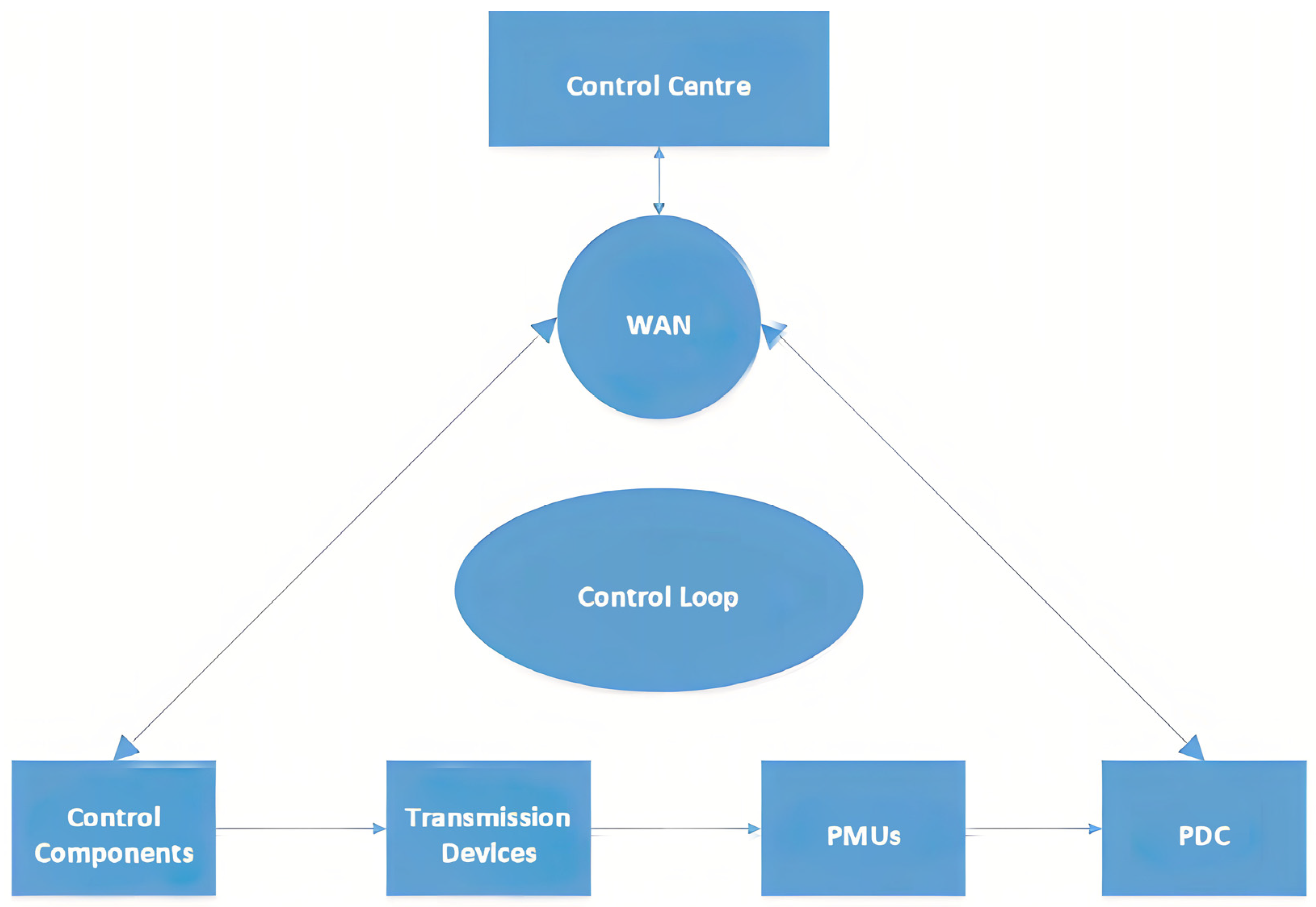
Power systems have four sections. Transmission, distribution, consumption, and transmission are the energy system’s foundation. It transmits power from the generator to the consumption center, often across miles and miles. Field detectors monitor the transmission network’s breakers and transformers. In Synchrophasor systems, field sensing uses PMUs. GPS signals are used to synchronize PMU data to UTC for continuous tracking. Phasor data concentration devices (PDCs) use WANs to transport Synchrophasor observations from temPMUs to the control center. Synchrophasor-based WAMS require PDCs and other PMUs. SCADA field sensors collect data every few seconds. WAMS use Synchrophasor technology to measure the data transfer system at 30–120 samples per second, quicker than SCADA. PDCs gather high-resolution measurement data for system status evaluation. The control facility uses complex algorithms to make actual time-field element control decisions. Controlling the loop ellipse centralized control lets system protection components detect and respond to disturbances [61]. Field sensors monitor transmission system components like breakers and transformers. A Synchrophasor system, in this particular case as shown in Figure 1.

The control center sends command data, and the IDEs send time-synchronized audit data. It is a finite-state machine. A control center command documented in the control center panel will induce a system state shift later. Breakers, relays that operate, and cables for transmission alter behavior over time, which changes the system state. Hardware logs record every modification. Temporal-state transitions are observed and measured data changes [62,63].

3.7. The Freshwater Reservoir

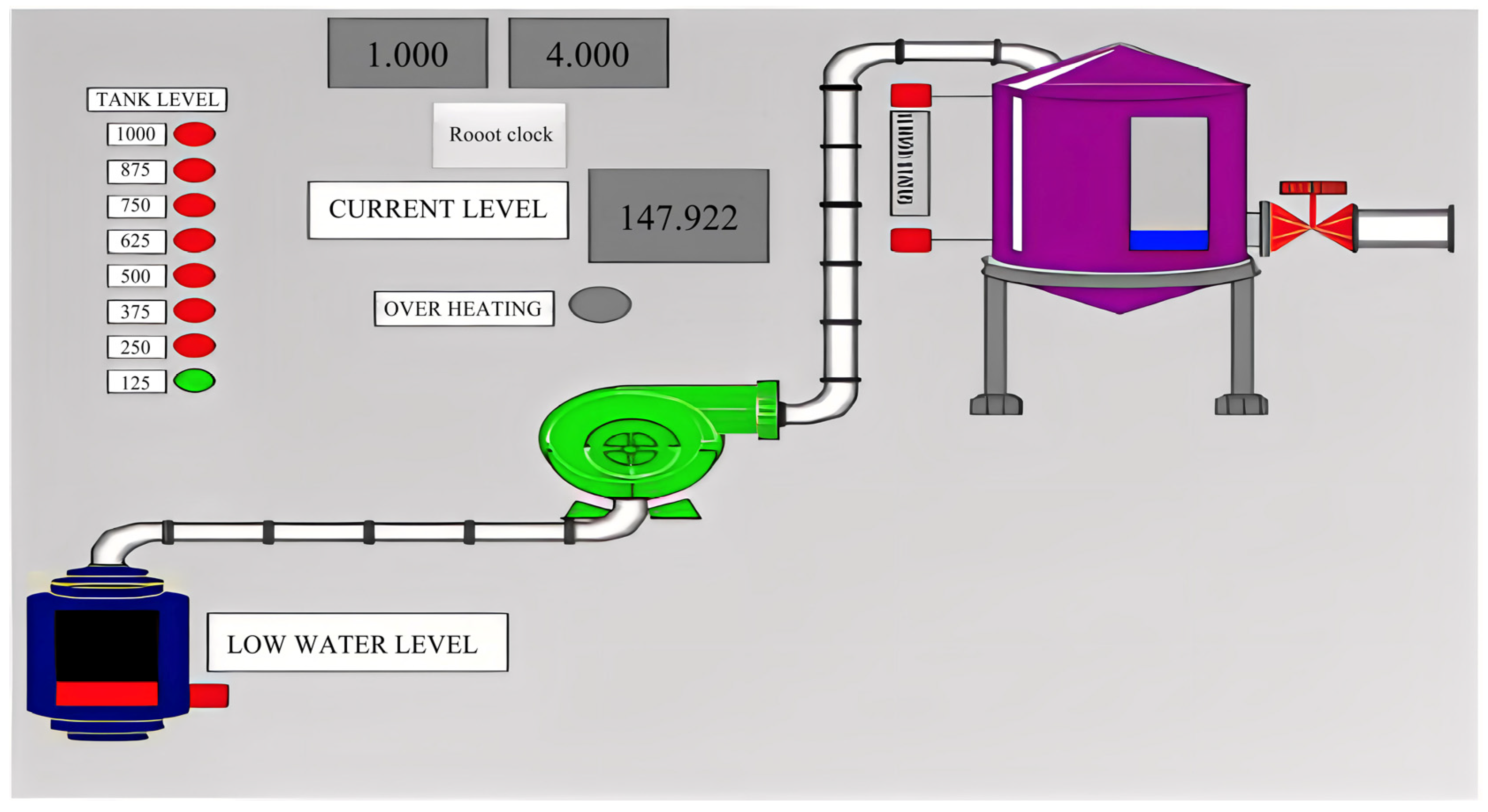
An RS-232 network data logger monitored and stored MODBUS traffic from the liquid storage vessel record. The authors of this paper first modeled gas pipeline functionality and water-holding container SCADA networks. Instead, we apply Ian Turnipseed’s upgraded gas pipeline dataset. The water reservoir’s management system mimics petrochemical manufacturing sector storage vessels for oil because the water-filled tank was developed for oil storage facilities. The tank has a main holding tank, an additional reservoir for the water container, and a pump that is used to move fluid out of the secondary reservoir to the main tank. A gravity-operated manually operated relief valve operates to allow liquid to pass from the main tank to the supplementary tank. In addition, a gauge is provided to measure the main tank’s capacity. Water exits the main tank and fills the additional tank. It uses closed-loop reservoir control. The water-holding system control method and factors of the system work correctly if the answer code for a function matches the given command’s functional code. Error response sub-function codes are the command function code plus 0 × 80. The system measures the water reservoir level. The unsophisticated and advanced malicious response injection assaults changed the predicted measuring results. During the test, a pump maintains the desired amount of water. The pump modes are on and off.

Human–machine interfacing (HMI) and the water reservoir system used by researchers are shown in Figure 2. The water tank was originally intended for oil storage. Moreover, its control system is based on those used in the petrochemical sector.

3.8. Gas Piping Statistics

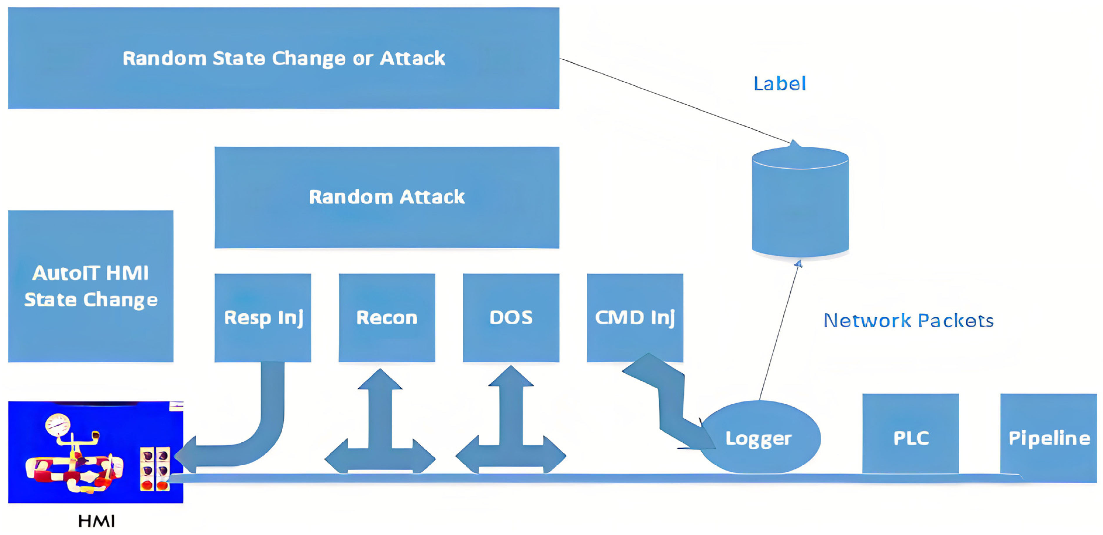
Sensors are device controls, an interaction system, and management controls that comprise this dataset’s gaseous pipeline structure. This paper illustrates the gas pipeline network that generated the information being studied and the HMI that controls it. Gas pipelines have two actuators and a type of pressure sensor. A hydraulic pump and solenoid govern the entire system’s mechanical process, while supervisory controls regulate pressure. Pipelines that carry gas are manual and automated. Managerial controls choose two pressure-maintenance systems in automated mode, as shown in Figure 3. First, the pumping mode setting controls pipeline pressure with the pump on/off controls. This approach maintains the system load. The solenoid mode is first. Solenoid-controlled relief valves regulate pressure in this system. This paper used a parametric and randomized approach to gather statistics. The threats were man-in-the-middle. The payload data includes gas pipeline state, options, and variables. These show system performance. These data are capable of identifying system outages and critical states. The dataset has 274,627 occurrences. Many aspects are uncertain since Modbus packets offer various details.

3.9. Analysis Techniques

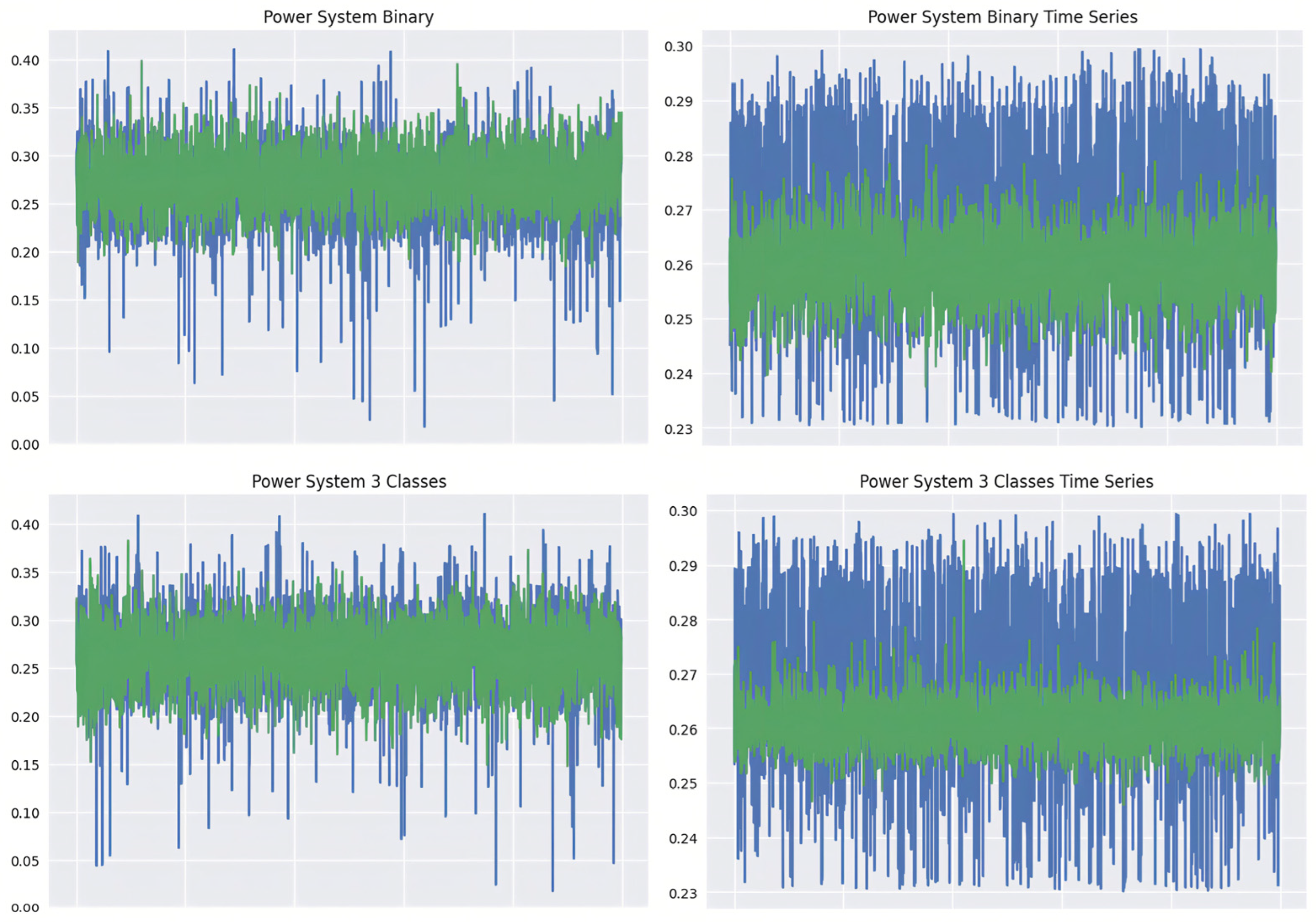
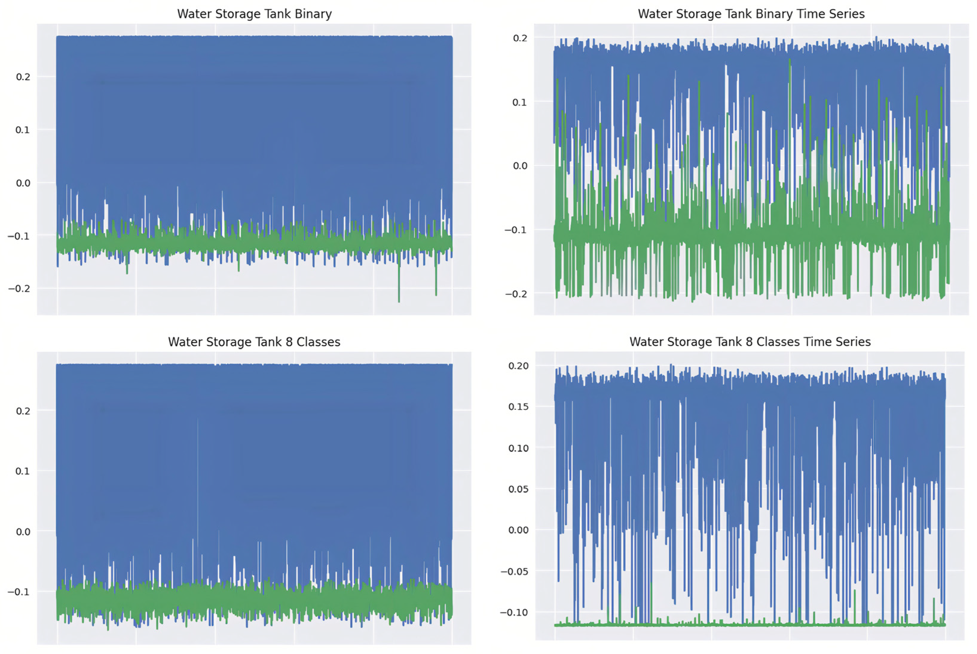
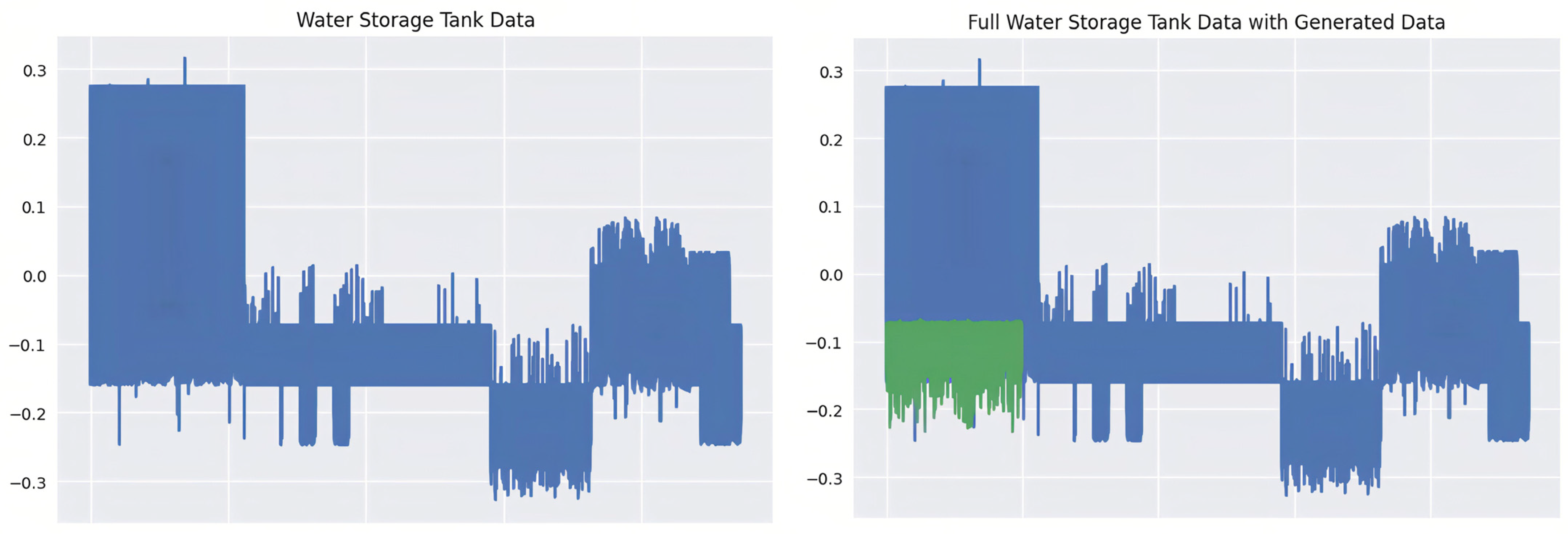
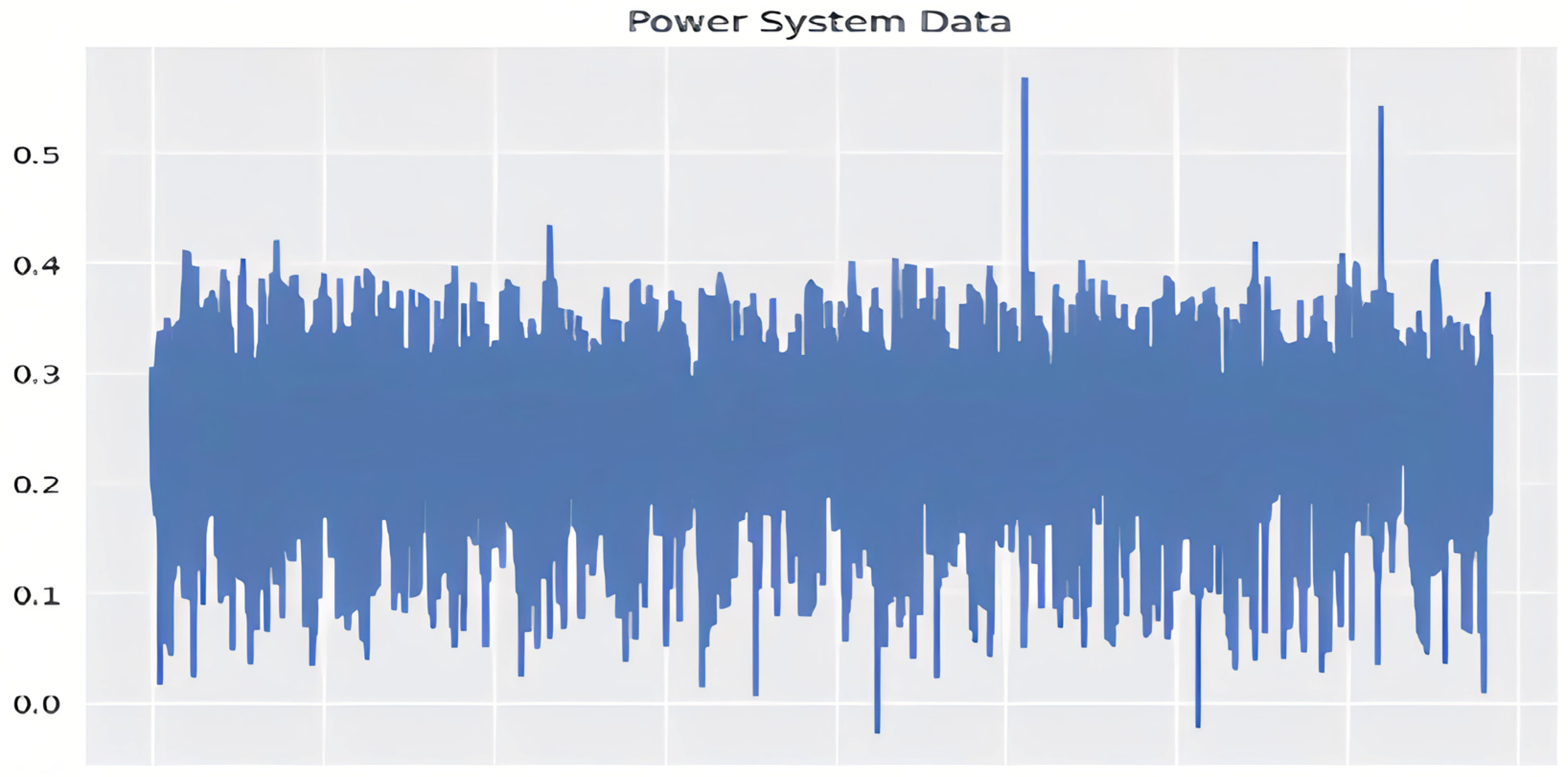
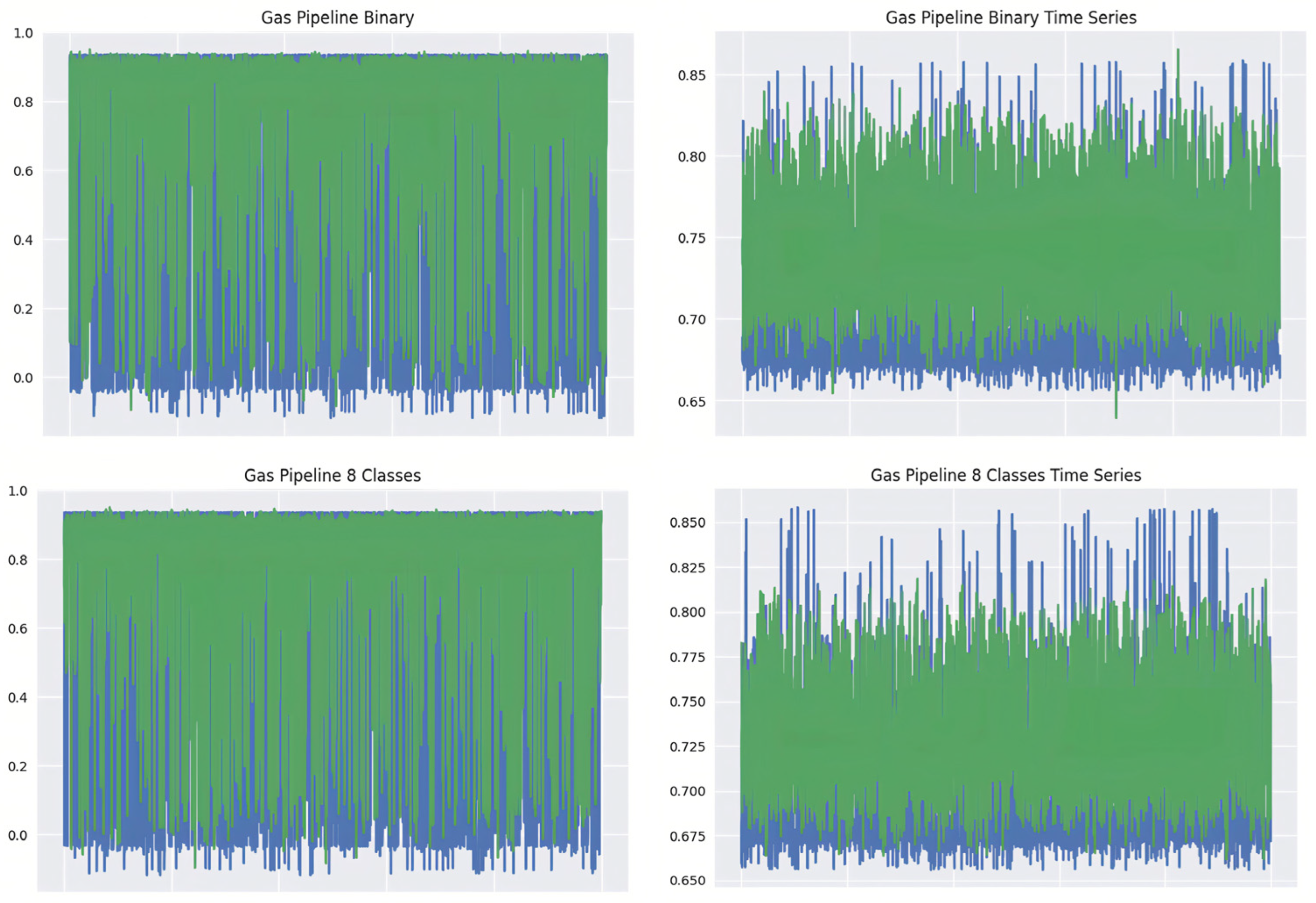
Data classification and generation using deep neural networks are the primary topics of this study. Common metrics for ICS identification of anomalies studies include precision, accuracy, recollection, F1-score, and the false-positive rate, all of which we examined. The generated network is a crucial component of our study. The generative network first generates samples of data based on its learned distribution of the probability of the original dataset. The next step is to assess the degree of similarity between the generated data and the source data.

We will compare the produced and original datasets using statistical measures like mean and variance. This is because, during model training, the mean serves as the loss function for the generator. A zero-mean, one-variance Gaussian noise was utilized to generate the dataset. The second method involves taking a random sample of 5000 data points and plotting them against 5000 original datasets. This will provide a visual summary of the created data’s resemblance to the original data [64].

This report focuses on major industries, including the electric power industry and water storage facilities. These fields rely substantially on ICS for their operations, and they are vital parts of society’s crucial infrastructure. This study prioritizes the protection of critical services by tackling cybersecurity concerns within these domains while also minimizing potential risks. A dedication to using cutting-edge technologies to deal with ICS risks is also reflected in the emphasis on developing and deploying neural systems in cybersecurity, in particular, residual neural networks. The detection of anomalies and breaches in ICS settings can benefit from residual neural networks’ superior performance in deep learning tasks. This exemplifies the authors’ commitment to leading the field of cybersecurity and using cutting-edge methods to safeguard vital networks and systems. Overall, this paper’s emphasis on key sectors and the utilization of cutting-edge technology like neural networks demonstrate a proactive approach to protecting ICS, which is essential in the face of constantly shifting cyber threats.

4. Results

Studies will compare the actual information set to the created dataset in terms of average and variance (with the exception of the MNIST data). It is assumed that the average variation comparing the actual data and the data that are generated will be small, as the mean is Wasserstein, which was utilized for distance training during the creation of the network. A selected number of 5000 records was plotted alongside the original and simulated datasets. All of the experimental findings are discussed here. The set of data will determine the divisions and segments. The data shown here are the product of 454 separate trials. Class imbalance can alter the model’s accuracy, which is problematic for industrial control systems because some risks may be much more uncommon than others. Different methods were used to try and lessen the impact of this problem. The dataset was made more equitable with the aid of oversampling methods like the synthetic minority over-sampling technique (SMOTE), which artificially increased the size of the minority class samples. Also, the model’s performance was judged using a wider range of measures, such as the F1-score and area under the receiver operating property curve (AUC-ROC), to account for situations in which classes are not equally represented. Collectively, these techniques improved the model’s capacity to identify and categorize dangers in ICS and SCADA environments [65].

4.1. Outcomes of the Power System

Table 1. Results for binary non-time-series power systems data.

Cutoff	Numbers	Precision	Recall	F1-Score	Accuracy	FP
0.1	0	0.55	0.53	0.34	0.36	0.48
	10,000	0.63	0.70	0.62	0.70	0.36
	20,000	0.62	0.66	0.63	0.66	0.41
	30,000	0.64	0.71	0.61	0.71	0.32
	40,000	0.61	0.67	0.62	0.67	0.44
	50,000	0.64	0.70	0.62	0.70	0.34
0.2	0	0.64	0.64	0.64	0.64	0.40
	10,000	0.64	0.69	0.65	0.69	0.35
	20,000	0.65	0.71	0.64	0.71	0.31
	30,000	0.67	0.71	0.64	0.71	0.25
	40,000	0.66	0.71	0.61	0.71	0.28
	50,000	0.66	0.71	0.63	0.71	0.27
0.3	0	0.64	0.65	0.65	0.65	0.39
	10,000	0.67	0.71	0.62	0.71	0.24
	20,000	0.66	0.71	0.64	0.71	0.30
	30,000	0.67	0.71	0.65	0.71	0.27
	40,000	0.64	0.69	0.65	0.69	0.35
	50,000	0.66	0.71	0.63	0.71	0.27
0.4	0	0.64	0.64	0.64	0.64	0.40
	10,000	0.67	0.71	0.65	0.71	0.27
	20,000	0.67	0.71	0.63	0.71	0.25
	30,000	0.65	0.70	0.65	0.70	0.33
	40,000	0.66	0.71	0.65	0.71	0.30
	50,000	0.67	0.71	0.61	0.70	0.24
0.5	0	0.65	0.69	0.66	0.69	0.34
	10,000	0.65	0.63	0.64	0.62	0.39
	20,000	0.66	0.71	0.65	0.71	0.28
	30,000	0.65	0.69	0.65	0.69	0.34
	40,000	0.65	0.69	0.66	0.69	0.33
	50,000	0.65	0.69	0.65	0.69	0.35
0.6	0	0.66	0.53	0.54	0.53	0.43
	10,000	0.65	0.66	0.65	0.66	0.37
	20,000	0.67	0.71	0.65	0.71	0.26
	30,000	0.67	0.71	0.65	0.71	0.26
	40,000	0.66	0.71	0.64	0.71	0.28
	50,000	0.67	0.72	0.64	0.71	0.25
0.7	0	0.64	0.65	0.65	0.65	0.39
	10,000	0.65	0.66	0.66	0.66	0.37
	20,000	0.67	0.71	0.65	0.71	0.27
	30,000	0.67	0.71	0.64	0.71	0.26
	40,000	0.66	0.69	0.66	0.68	0.34
	50,000	0.66	0.71	0.65	0.71	0.29
0.8	0	0.68	0.45	0.44	0.45	0.45
	10,000	0.65	0.66	0.65	0.66	0.37
	20,000	0.65	0.64	0.64	0.63	0.38
	30,000	0.66	0.70	0.66	0.70	0.31
	40,000	0.67	0.71	0.66	0.70	0.30
	50,000	0.66	0.70	0.66	0.70	0.31

displays the outcomes of experiments conducted using binary non-time-sequence information from the electric power system. Adding the produced data to the starting point data during the testing process increases the accuracy of the model. The created data seem to contribute less than the actual information. Nevertheless, models can reach 71% correctness.

Table 2. Results for binary time-series power systems data.

Cutoff	Numbers	Precision	Recall	F1-Score	Accuracy	FP
0.1	0	0.84	0.82	0.83	0.82	0.17
	10,000	0.88	0.87	0.87	0.87	0.12
	20,000	0.87	0.87	0.87	0.86	0.11
	25,000	0.84	0.85	0.84	0.85	0.09
0.2	0	0.86	0.75	0.77	0.75	0.25
	10,000	0.92	0.92	0.92	0.92	0.04
	20,000	0.89	0.89	0.89	0.89	0.08
	25,000	0.91	0.91	0.91	0.91	0.06
0.3	0	0.88	0.87	0.88	0.87	0.12
	10,000	0.94	0.94	0.94	0.94	0.05
	20,000	0.91	0.91	0.90	0.91	0.03
	25,000	0.92	0.91	0.91	0.91	0.07
0.4	0	0.90	0.86	0.86	0.86	0.16
	10,000	0.96	0.96	0.96	0.96	0.03
	20,000	0.90	0.86	0.86	0.86	0.16
	25,000	0.96	0.96	0.96	0.96	0.03
0.5	0	0.92	0.92	0.92	0.92	0.07
	10,000	0.95	0.95	0.95	0.95	0.05
	20,000	0.96	0.96	0.96	0.96	0.02
	25,000	0.98	0.97	0.97	0.97	0.02
0.6	0	0.96	0.96	0.96	0.96	0.04
	10,000	0.92	0.88	0.89	0.88	0.14
	20,000	0.97	0.97	0.97	0.97	0.02
	25,000	0.98	0.97	0.97	0.97	0.01
0.7	0	0.96	0.96	0.96	0.96	0.04
	10,000	0.97	0.97	0.97	0.97	0.03
	20,000	0.98	0.98	0.98	0.98	0.01
	25,000	0.97	0.97	0.97	0.97	0.01
0.8	0	0.94	0.93	0.93	0.93	0.08
	10,000	0.98	0.98	0.98	0.98	0.02
	20,000	0.99	0.99	0.99	0.99	0.008
	25,000	0.97	0.97	0.97	0.97	0.03

displays the experimental outcomes of the binary time-series data gathered from the power systems. The created data enhanced the model’s effectiveness in all cases. The produced data can boost accuracy by 17%. However, the original data improved efficiency the most.

Table 3. Results for multi-class non-time-series power system data.

Cutoff	Number	Precision	Recall	F1-Score	Accuracy	FP
0.1	0	0.62	0.50	0.52	0.50	0.46
	10,000	0.63	0.69	0.62	0.69	0.56
	20,000	0.64	0.70	0.63	0.70	0.49
	30,000	0.62	0.68	0.62	0.68	0.55
	40,000	0.60	0.68	0.61	0.67	0.60
	50,000	0.63	0.67	0.61	0.67	0.64
0.2	0	0.63	0.64	0.63	0.64	0.43
	10,000	0.65	0.71	0.61	0.71	0.60
	20,000	0.68	0.71	0.62	0.71	0.57
	30,000	0.66	0.71	0.62	0.70	0.57
	40,000	0.66	0.71	0.63	0.71	0.51
	50,000	0.66	0.71	0.62	0.70	0.53
0.3	0	0.62	0.65	0.63	0.65	0.43
	10,000	0.66	0.71	0.63	0.71	0.47
	20,000	0.66	0.71	0.64	0.71	0.46
	30,000	0.65	0.71	0.64	0.71	0.46
	40,000	0.66	0.70	0.64	0.70	0.51
	50,000	0.67	0.71	0.62	0.71	0.52
0.4	0	0.63	0.53	0.56	0.53	0.46
	10,000	0.65	0.70	0.65	0.70	0.44
	20,000	0.66	0.71	0.64	0.71	0.45
	30,000	0.66	0.71	0.63	0.71	0.49
	40,000	0.68	0.71	0.61	0.71	0.64
	50,000	0.66	0.71	0.63	0.71	0.47
0.5	0	0.65	0.70	0.65	0.70	0.42
	10,000	0.64	0.70	0.63	0.70	0.50
	20,000	0.57	0.37	0.36	0.71	0.47
	30,000	0.66	0.70	0.64	0.69	0.49
	40,000	0.67	0.71	0.64	0.71	0.44
	50,000	0.66	0.71	0.64	0.71	0.46
0.6	0	0.64	0.55	0.57	0.54	0.45
	10,000	0.65	0.70	0.64	0.70	0.46
	20,000	0.66	0.71	0.64	0.71	0.44
	30,000	0.66	0.71	0.63	0.71	0.49
	40,000	0.65	0.70	0.65	0.70	0.42
	50,000	0.70	0.71	0.61	0.71	0.63
0.7	0	0.64	0.61	0.62	0.60	0.42
	10,000	0.65	0.71	0.64	0.71	0.45
	20,000	0.65	0.70	0.65	0.69	0.45
	30,000	0.67	0.72	0.64	0.71	0.43
	40,000	0.66	0.71	0.65	0.71	0.44
	50,000	0.66	0.70	0.64	0.70	0.44
0.8	0	0.64	0.54	0.56	0.54	0.43
	10,000	0.65	0.69	0.66	0.69	0.41
	20,000	0.65	0.70	0.65	0.70	0.44
	30,000	0.67	0.72	0.63	0.71	0.48
	40,000	0.68	0.72	0.63	0.71	0.48
	50,000	0.68	0.71	0.64	0.71	0.44

displays the outcomes of studies conducted using data from power systems that include many classes but no time series. Adding new data usually enhances the network’s accuracy, but it raises the percentage of false positives in this dataset. Similar to Table 1, the neural network looks to have a 71% precision limit.

Table 4. Results for multi-class time-series power system data.

Cutoff	Numbers	Precision	Recall	F1-Score	Accuracy	FP
0.1	0	0.87	0.81	0.82	0.81	0.19
	10,000	0.87	0.87	0.86	0.87	0.07
	20,000	0.76	0.78	0.76	0.77	0.20
	25,000	0.88	0.88	0.87	0.88	0.10
0.2	0	0.93	0.92	0.92	0.92	0.08
	10,000	0.92	0.92	0.92	0.92	0.07
	20,000	0.95	0.95	0.95	0.95	0.04
	25,000	0.90	0.90	0.90	0.90	0.06
0.3	0	0.95	0.94	0.94	0.94	0.07
	10,000	0.99	0.96	0.98	0.96	0.04
	20,000	0.99	0.93	0.96	0.93	0.07
	25,000	0.96	0.96	0.96	0.96	0.02
0.4	0	0.95	0.94	0.94	0.94	0.07
	10,000	0.97	0.97	0.97	0.97	0.02
	20,000	0.97	0.97	0.97	0.97	0.02
	25,000	0.99	0.95	0.97	0.95	0.05
0.5	0	0.97	0.97	0.97	0.97	0.03
	10,000	0.98	0.98	0.98	0.98	0.01
	20,000	0.98	0.98	0.98	0.98	0.01
	25,000	0.98	0.98	0.98	0.98	0.02
0.6	0	0.98	0.98	0.98	0.98	0.02
	10,000	0.98	0.98	0.98	0.98	0.02
	20,000	0.98	0.98	0.98	0.98	0.01
	25,000	0.98	0.98	0.98	0.98	0.01
0.7	0	0.99	0.98	0.98	0.98	0.02
	10,000	0.98	0.98	0.98	0.98	0.02
	20,000	0.97	0.97	0.97	0.97	0.03
	25,000	0.99	0.99	0.99	0.99	0.01
0.8	0	0.97	0.97	0.97	0.97	0.03
	10,000	0.98	0.98	0.98	0.98	0.01
	20,000	0.98	0.98	0.98	0.98	0.01
	25,000	0.99	0.99	0.99	0.99	0.01

shows the multi-class time series of power system database trial outcomes. Padding the initial information with the produced data regularly increases network speed. The generated data helped the network attain 99% accuracy continuously [66].

Figure 4 shows genuine data in blue and created statistics in green. The original data were obtained from the power system initial test. All results have decreased variance. Both the initial and produced data have similar means. The graph indicates that the initial dataset is more “random” than the created data, despite the fact that the average of the time period dataset is similar.

4.2. Outcomes of the Water Storage Reservoir

Table 5. Results for binary non-time-series water storage tank data.

Cutoff	Numbers	Precision	Recall	F1-Score	Accuracy	FP
0.1	0	0.92	0.90	0.90	0.90	0.0004
	10,000	0.89	0.87	0.86	0.87	0.00
	20,000	0.91	0.90	0.89	0.90	0.0004
	30,000	0.91	0.90	0.89	0.90	0.0003
	40,000	0.91	0.90	0.89	0.90	0.0004
	50,000	0.91	0.90	0.89	0.90	0.0004
0.2	0	0.92	0.91	0.90	0.90	0.0004
	10,000	0.89	0.87	0.86	0.87	0.0
	20,000	0.89	0.87	0.86	0.87	0.0
	30,000	0.89	0.87	0.86	0.87	0.0
	40,000	0.92	0.90	0.90	0.90	0.0004
	50,000	0.89	0.87	0.86	0.87	0.0
0.3	0	0.92	0.90	0.90	0.90	0.0004
	10,000	0.89	0.87	0.86	0.87	0.0
	20,000	0.91	0.90	0.90	0.90	0.0003
	30,000	0.92	0.91	0.90	0.90	0.0005
	40,000	0.92	0.90	0.90	0.90	0.0004
	50,000	0.91	0.90	0.90	0.90	0.0004
0.4	0	0.91	0.90	0.90	0.90	0.0004
	10,000	0.90	0.88	0.86	0.88	0.0
	20,000	0.91	0.90	0.90	0.90	0.0005
	30,000	0.92	0.91	0.90	0.90	0.0005
	40,000	0.92	0.90	0.90	0.90	0.0005
	50,000	0.92	0.91	0.90	0.90	0.0004
0.5	0	0.89	0.87	0.86	0.87	0.0
	10,000	0.89	0.87	0.86	0.87	0.0
	20,000	0.89	0.87	0.86	0.87	0.0
	30,000	0.92	0.90	0.90	0.90	0.0006
	40,000	0.92	0.90	0.90	0.90	0.0007
	50,000	0.92	0.91	0.90	0.90	0.0005
0.6	0	0.92	0.90	0.90	0.90	0.0006
	10,000	0.89	0.87	0.86	0.87	0.0
	20,000	0.91	0.90	0.90	0.90	0.0004
	30,000	0.92	0.90	0.90	0.90	0.0006
	40,000	0.91	0.90	0.90	0.90	0.0004
	50,000	0.92	0.90	0.90	0.90	0.0005
0.7	0	0.89	0.87	0.86	0.87	0.0
	10,000	0.92	0.90	0.90	0.90	0.0005
	20,000	0.92	0.90	0.90	0.90	0.0003
	30,000	0.91	0.90	0.90	0.90	0.0003
	40,000	0.92	0.91	0.90	0.91	0.0004
	50,000	0.92	0.90	0.90	0.90	0.001
0.8	0	0.92	0.91	0.90	0.90	0.0005
	10,000	0.90	0.88	0.87	0.88	0.0
	20,000	0.91	0.90	0.89	0.90	0.0001
	30,000	0.89	0.89	0.88	0.89	0.08
	40,000	0.91	0.90	0.89	0.90	0.0002
	50,000	0.87	0.87	0.87	0.87	0.18

displays the test outcomes of the binary non-time-sequence water holding tank database. When compared with data from power systems, the outcome is inconsistent with expectations. However, the numbers demonstrate that the network consistently returns results within a 90% confidence interval.

Table 6. Results for binary time-series water storage tank data.

Cutoff	Numbers	Precision	Recall	F1-Score	Accuracy	FP
0.1	0	0.77	0.63	0.65	0.63	0.39
	10,000	0.78	0.79	0.78	0.79	0.30
	20,000	0.78	0.79	0.78	0.79	0.30
	25,000	0.78	0.79	0.78	0.79	0.30
0.2	0	0.78	0.79	0.78	0.79	0.30
	10,000	0.78	0.79	0.78	0.79	0.30
	20,000	0.78	0.79	0.78	0.79	0.30
	25,000	0.78	0.79	0.78	0.79	0.30
0.3	0	0.78	0.79	0.78	0.79	0.30
	10,000	0.76	0.68	0.69	0.68	0.38
	20,000	0.78	0.79	0.78	0.79	0.30
	25,000	0.77	0.78	0.78	0.78	0.32
0.4	0	0.78	0.79	0.78	0.79	0.30
	10,000	0.76	0.75	0.75	0.75	0.35
	20,000	0.77	0.78	0.78	0.78	0.31
	25,000	0.78	0.79	0.78	0.79	0.30
0.5	0	0.78	0.79	0.78	0.79	0.30
	10,000	0.78	0.79	0.78	0.79	0.30
	20,000	0.78	0.79	0.78	0.79	0.30
	25,000	0.77	0.78	0.77	0.78	0.32
0.6	0	0.78	0.79	0.78	0.79	0.30
	10,000	0.76	0.76	0.76	0.76	0.34
	20,000	0.77	0.77	0.77	0.77	0.32
	25,000	0.76	0.76	0.76	0.76	0.35
0.7	0	0.78	0.79	0.78	0.79	0.30
	10,000	0.78	0.79	0.78	0.79	0.30
	20,000	0.78	0.79	0.78	0.79	0.30
	25,000	0.78	0.79	0.78	0.79	0.31
0.8	0	0.78	0.63	0.65	0.63	0.39
	10,000	0.78	0.79	0.78	0.79	0.30
	20,000	0.78	0.79	0.78	0.79	0.30
	25,000	0.78	0.79	0.78	0.79	0.30

displays the experimental results of binary time-series data from water holding tanks. The outcomes are consistent with those shown in the case of binary, non-time-series data. The data generation does not help the system in any way.

Table 7. Results for 8-class non-time-series water storage tank data.

Cutoff	Numbers	Precision	Recall	F1-Score	Accuracy	FP
0.1	0	0.82	0.91	0.86	0.90	0.002
	10,000	0.85	0.72	0.77	0.72	0.38
	20,000	0.84	0.75	0.79	0.75	0.36
	30,000	0.71	0.56	0.61	0.56	0.50
	40,000	0.69	0.62	0.65	0.62	0.50
	50,000	0.69	0.57	0.62	0.57	0.50
0.2	0	0.82	0.90	0.86	0.90	0.002
	10,000	0.83	0.76	0.79	0.76	0.35
	20,000	0.84	0.76	0.79	0.75	0.36
	30,000	0.84	0.66	0.73	0.66	0.40
	40,000	0.83	0.66	0.72	0.66	0.40
	50,000	0.70	0.60	0.63	0.60	0.50
0.3	0	0.82	0.90	0.86	0.90	0.002
	10,000	0.84	0.81	0.82	0.81	0.31
	20,000	0.85	0.75	0.78	0.74	0.36
	30,000	0.84	0.79	0.81	0.79	0.33
	40,000	0.85	0.69	0.75	0.69	0.39
	50,000	0.84	0.74	0.78	0.74	0.36
0.4	0	0.82	0.90	0.86	0.90	0.006
	10,000	0.84	0.75	0.78	0.75	0.36
	20,000	0.84	0.75	0.79	0.75	0.36
	30,000	0.84	0.77	0.79	0.77	0.35
	40,000	0.84	0.79	0.81	0.79	0.33
	50,000	0.85	0.73	0.77	0.73	0.37
0.5	0	0.82	0.90	0.86	0.90	0.002
	10,000	0.84	0.77	0.80	0.77	0.34
	20,000	0.84	0.76	0.79	0.76	0.35
	30,000	0.83	0.83	0.83	0.83	0.27
	40,000	0.85	0.72	0.77	0.72	0.38
	50,000	0.85	0.73	0.78	0.73	0.37
0.6	0	0.82	0.90	0.86	0.90	0.006
	10,000	0.84	0.78	0.81	0.78	0.33
	20,000	0.83	0.89	0.85	0.89	0.09
	30,000	0.84	0.82	0.82	0.82	0.30
	40,000	0.84	0.76	0.79	0.76	0.35
	50,000	0.83	0.78	0.80	0.77	0.35
0.7	0	0.82	0.90	0.86	0.90	0.002
	10,000	0.83	0.84	0.83	0.84	0.25
	20,000	0.84	0.75	0.79	0.75	0.36
	30,000	0.85	0.73	0.78	0.73	0.37
	40,000	0.84	0.79	0.81	0.79	0.32
	50,000	0.85	0.75	0.79	0.75	0.36
0.8	0	0.82	0.90	0.86	0.90	0.002
	10,000	0.84	0.76	0.79	0.76	0.35
	20,000	0.84	0.78	0.80	0.77	0.34
	30,000	0.84	0.80	0.81	0.80	0.31
	40,000	0.84	0.76	0.79	0.75	0.36
	50,000	0.85	0.75	0.78	0.74	0.36

displays the results of an eight-class classification of data from water storage tanks. Again, the created data do not boost the efficiency of the model, as demonstrated by the results. All of the preceding results are consistent with the data from water storage tanks. The incorporation of the generated data does not result in any appreciable performance boost.

Figure 5 indicates that the data produced differs greatly from the first dataset. Figure 6 illustrates this numerical similarity but graphical and visual disparity. Figure 6 graphs the whole water-holding tank dataset. Similar to the additional datasets, the data are inconsistent. Figure 7 shows the electric power system dataset for comparison. Figure 6 resembles time-series data, in contrast to Figure 7. Thus, the data collection’s shape makes it visually distinct despite its understandable mean and variance.

4.3. Outcomes of the Gas Pipeline

Table 8. Results for 8-class time-series water storage tank data.

Cutoff	Numbers	Precision	Recall	F1-Score	Accuracy	FP
0.1	0	0.70	0.79	0.74	0.78	0.31
	10,000	0.70	0.79	0.74	0.79	0.30
	20,000	0.70	0.79	0.74	0.79	0.30
	25,000	0.70	0.79	0.74	0.79	0.30
0.2	0	0.70	0.78	0.74	0.78	0.31
	10,000	0.70	0.79	0.74	0.79	0.30
	20,000	0.70	0.79	0.74	0.79	0.30
	25,000	0.70	0.79	0.74	0.79	0.30
0.3	0	0.70	0.77	0.73	0.77	0.32
	10,000	0.70	0.79	0.74	0.79	0.30
	20,000	0.70	0.79	0.74	0.79	0.30
	25,000	0.70	0.79	0.74	0.79	0.30
0.4	0	0.70	0.78	0.74	0.78	0.31
	10,000	0.70	0.79	0.74	0.79	0.30
	20,000	0.71	0.79	0.74	0.79	0.30
	25,000	0.70	0.79	0.74	0.79	0.30
0.5	0	0.70	0.79	0.74	0.78	0.31
	10,000	0.70	0.79	0.74	0.79	0.30
	20,000	0.70	0.79	0.74	0.79	0.30
	25,000	0.70	0.79	0.74	0.79	0.30
0.6	0	0.70	0.77	0.73	0.77	0.33
	10,000	0.79	0.79	0.74	0.79	0.30
	20,000	0.70	0.79	0.74	0.79	0.30
	25,000	0.70	0.79	0.74	0.79	0.29
0.7	0	0.70	0.78	0.73	0.77	0.32
	10,000	0.75	0.79	0.74	0.78	0.31
	20,000	0.70	0.79	0.74	0.79	0.30
	25,000	0.71	0.79	0.74	0.79	0.30
0.8	0	0.71	0.79	0.74	0.79	0.31
	10,000	0.74	0.79	0.75	0.79	0.30
	20,000	0.70	0.79	0.74	0.79	0.30
	25,000	0.71	0.79	0.74	0.79	0.30

shows the binary non-time-sequence gas pipeline data outcomes from experiments. Attaching data improved efficiency. The network usually outperforms the original dataset.

Table 9. Results for binary non-time-series gas pipeline data.

Cutoff	Numbers	Precision	Recall	F1-Score	Accuracy	FP
0.1	0	0.82	0.61	0.64	0.60	0.40
	10,000	0.86	0.83	0.79	0.83	0.04
	20,000	0.79	0.74	0.76	0.74	0.38
	30,000	0.83	0.62	0.65	0.62	0.40
	40,000	0.76	0.37	0.36	0.37	0.45
	50,000	0.82	0.62	0.65	0.61	0.40
0.2	0	0.82	0.62	0.65	0.62	0.40
	10,000	0.86	0.83	0.78	0.83	0.005
	20,000	0.83	0.62	0.65	0.62	0.40
	30,000	0.85	0.83	0.80	0.83	0.07
	40,000	0.83	0.62	0.65	0.62	0.40
	50,000	0.82	0.61	0.64	0.61	0.40
0.3	0	0.83	0.62	0.65	0.62	0.40
	10,000	0.83	0.62	0.65	0.61	0.40
	20,000	0.82	0.62	0.65	0.62	0.40
	30,000	0.74	0.71	0.72	0.71	0.43
	40,000	0.82	0.62	0.65	0.62	0.40
	50,000	0.77	0.38	0.37	0.38	0.45
0.4	0	0.84	0.82	0.76	0.82	0.08
	10,000	0.83	0.62	0.65	0.62	0.40
	20,000	0.83	0.62	0.65	0.62	0.40
	30,000	0.83	0.63	0.66	0.62	0.40
	40,000	0.86	0.83	0.79	0.83	0.03
	50,000	0.78	0.37	0.36	0.37	0.44
0.5	0	0.83	0.61	0.64	0.61	0.40
	10,000	0.05	0.22	0.08	0.21	-
	20,000	0.83	0.82	0.76	0.81	0.10
	30,000	0.86	0.83	0.78	0.83	0.006
	40,000	0.78	0.74	0.75	0.74	0.39
	50,000	0.78	0.37	0.35	0.37	0.44
0.6	0	0.81	0.62	0.65	0.61	0.41
	10,000	0.85	0.83	0.79	0.83	0.04
	20,000	0.83	0.62	0.65	0.62	0.40
	30,000	0.77	0.77	0.77	0.77	0.37
	40,000	0.82	0.62	0.65	0.62	0.40
	50,000	0.83	0.61	0.64	0.61	0.40
0.7	0	0.83	0.63	0.66	0.63	0.39
	10,000	0.83	0.63	0.66	0.62	0.39
	20,000	0.83	0.62	0.65	0.62	0.39
	30,000	0.85	0.83	0.79	0.83	0.05
	40,000	0.83	0.63	0.66	0.63	0.39
	50,000	0.85	0.83	0.79	0.83	0.07
0.8	0	0.77	0.72	0.74	0.72	0.40
	10,000	0.78	0.74	0.75	0.74	0.39
	20,000	0.81	0.82	0.79	0.82	0.22
	30,000	0.80	0.75	0.77	0.75	0.38
	40,000	0.83	0.63	0.66	0.62	0.39
	50,000	0.83	0.62	0.65	0.62	0.39

shows binary periods in the gas pipeline dataset’s outcomes from experiments. If the network performs poorly on the initial dataset, adding the produced data does not improve performance. The generated data do not help network performance.

Table 10. Results for binary time-series gas pipeline data.

Cutoff	Numbers	Precision	Recall	F1-Score	Accuracy	FP
0.1	0	0.74	0.61	0.65	0.61	0.44
	10,000	0.72	0.68	0.70	0.68	0.44
	20,000	0.74	0.64	0.67	0.64	0.43
	25,000	0.71	0.70	0.71	0.70	0.45
0.2	0	0.74	0.64	0.67	0.64	0.44
	10,000	0.73	0.66	0.68	0.65	0.44
	20,000	0.74	0.67	0.69	0.66	0.43
	25,000	0.73	0.65	0.68	0.65	0.44
0.3	0	0.74	0.65	0.68	0.65	0.44
	10,000	0.74	0.58	0.62	0.58	0.44
	20,000	0.74	0.63	0.66	0.44	0.44
	25,000	0.72	0.70	0.71	0.69	0.44
0.4	0	0.73	0.68	0.70	0.67	0.44
	10,000	0.72	0.70	0.71	0.70	0.43
	20,000	0.75	0.64	0.67	0.64	0.43
	25,000	0.73	0.67	0.69	0.67	0.44
0.5	0	0.75	0.65	0.68	0.65	0.43
	10,000	0.74	0.68	0.70	0.67	0.43
	20,000	0.74	0.67	0.69	0.67	0.43
	25,000	0.73	0.67	0.69	0.66	0.44
0.6	0	0.75	0.65	0.68	0.65	0.43
	10,000	0.74	0.67	0.69	0.67	0.43
	20,000	0.74	0.68	0.70	0.68	0.43
	25,000	0.74	0.69	0.71	0.69	0.43
0.7	0	0.75	0.67	0.69	0.66	0.42
	10,000	0.75	0.67	0.70	0.67	0.43
	20,000	0.74	0.69	0.71	0.68	0.43
	25,000	0.75	0.63	0.67	0.63	0.43
0.8	0	0.74	0.68	0.70	0.67	0.43
	10,000	0.74	0.68	0.70	0.67	0.43
	20,000	0.76	0.61	0.64	0.60	0.43
	25,000	0.75	0.67	0.69	0.66	0.42

shows eight-class non-time-sequence gas pipeline data test outcomes. Data scarcity improves the original dataset. However, 10,000 generated data points work best when the threshold for data collection is greater than 0.5. Increasing the original data quality increases the data quality. Thus, performance improves with more original data. The study has to be confined to 0.1, 0.5, and then 0.8 cutoffs, 0, and 25,000 appended numbers.

Table 11. Results for 8-class time-series gas pipeline data.

Cutoff	Numbers	Precision	Recall	F1-Score	Accuracy	FP
0.1	0	0.66	0.72	0.69	0.72	0.50
	25,000	0.70	0.71	0.70	0.71	0.47
0.5	0	0.66	0.71	0.68	0.71	0.51
	25,000	0.62	0.31	0.40	0.30	0.54
0.8	0	0.65	0.72	0.68	0.72	0.52
	25,000	0.67	0.70	0.68	0.70	0.50

shows eight-class time-series gas piping data and experimental outcomes. The initial and produced data scored poorly in all scenarios. Computational and memory limitations shortened the testing period. This experiment’s storage and computation requirements are unrealistic.

Reliability was poor, and the majority of the networks aggregated with 90% precision. The data collection structure explains this. The average, variance, and general variations visually display how neural network algorithms distinguish groups. Since each class is unique, the machine learning system is able to distinguish with roughly 90% accuracy in most trials in this section of this paper.

The generated network can produce samples that are aesthetically comparable to the actual dataset, as demonstrated in Figure 8. In contrast with the previous datasets, however, the averages and variance here are not as close to their initial values. While the results show promise for the water reservoir and gas pipeline datasets, this study’s credibility has to be bolstered by integrating strong model validation methods. Cross-validation or testing on a separate dataset would be invaluable to validate the model’s generalization capabilities, notwithstanding the claimed accuracy of 71% in the water-based reservoir industry. In order to determine if the accuracy of the model is stable across datasets and scenarios, these validation techniques can be used. Furthermore, this study found discrepancies when comparing results to data from power systems, underscoring the necessity for thorough validation to comprehend the model’s behavior in various real-world settings. It is also important for honesty’s sake to note that the testing time was impacted by computational and memory constraints. In conclusion, including model validation metrics would strengthen the trustworthiness of this study and offer a more in-depth assessment of the model’s efficacy.

There are substantial real-world applications of the findings reported in this study. The precision could be useful in detecting anomalies in water storage tanks at an early stage, avoiding problems with water quality or costly infrastructure failures. However, the requirement for sector-specific fine-tuning is highlighted by the observed discrepancy when comparing data from power systems. The results raise concerns that the model’s efficacy may fall short of expectations in the context of gas pipeline observation, where dependability is of the utmost significance. Critical gas pipeline observation scenarios call for robust contingency plans and human involvement due to the low reliability and difficulties in generating exact results. In addition, the testing showed that there is a need to optimize resource utilization for real-world deployments due to computational and memory limits. To ensure the model can function efficiently in a business environment, real-world applications must think about how to work around these limitations. In conclusion, while the models show promise, their practical influence in water storage tank and gas pipeline tracking will depend on rigorous adaptation to the individual industry, addressing dependability concerns, and optimizing computing needs to suit practical requirements.

In computer security, a zero-day security hole is a flaw that is discovered by cybercriminals before the vendor is aware of it. Until the flaw is fixed, malicious actors can take advantage of it to compromise sensitive data or software. A zero-day attack is an exploit that targets a vulnerability with no known solution. Criminals conceal their actions by switching up the attack vector to foil traditional antivirus software. A zero-day exploit is a flaw in software that has not been made public and can be used by hackers to cause harm [67,68]. A security strategy must be implemented to protect against zero-day ransomware attacks, which is why safeguarding systems against such assaults is so crucial. The vicious circle of needing to rebuild the defense system only continues. Defenders can construct defense systems using data they already possess, which has not been requested or provided by attackers. For example, an adaptive defense system could be constructed as a means for detecting potential zero-day attacks. This system would involve gathering data to identify critical assets, monitoring processes (system calls), and making decisions to catch malicious behaviors associated with using the critical assets, which would check the security system’s load time and make it OS-independent [69].

5. Conclusions

This research concluded that the manufacturing industry’s essential area of controlling processes is increasingly at risk due to the widespread adoption of low-power sensors and Internet of Things (IoT) solutions. Cyberattacks on these industries have been highlighted, as has the lack of effective security systems, which leaves our electronic gadgets and infrastructure open to assault. Our approach combined data from three databases that track critically important infrastructure: those that keep track of power plants, water reservoirs, and gas lines. Key discoveries arose as we analyzed the collected dataset and performed preliminary statistical evaluations. In the scenario of electric power systems, where time-series information is unavailable, one of the important discoveries is that supplementing the dataset cannot always enhance the efficiency of systems already battling difficulties in the initial dataset. In addition, this study used information about water reservoirs to emphasize the significance of information accuracy when using more recent types of systems to generate samples. The fact that the created data replicated inconsistencies found in the original water reservoir dataset brought attention to the need for precise and reliable data. Finally, this study proved that feeding more data into neural networks greatly improved the effectiveness of the dataset. Overall performance often improves after being exposed to a wider variety of scenarios, including edge cases.

However, the scope of this endeavor has limitations that must be taken into account. For example, the study’s conclusions may not be readily transferable to other sectors due to its narrow focus on infrastructure. More research is needed on this important subject because this study did not even touch on the topic of implementing particular security mechanisms against cyberattacks. The goal of future research in this area should be to create and evaluate effective cybersecurity solutions that address the specific threats posed by low-power sensing and Internet of Things technologies in industrial settings.

References

1. Li, B.; Tan, Y.; Wu, A.-G.; Duan, G.-R. A Distributionally Robust Optimization Based Method for Stochastic Model Predictive Control. IEEE Trans. Automat Contr. 2021, 67, 5762–5776. [Google Scholar] [CrossRef]
2. Andreeva, O.; Gordeychik, S.; Gritsai, G.; Kochetova, O.; Potseluevskaya, E.; Sidorov, S.I.; Timorin, A.A. Industrial Control Systems Vulnerabilities Statistics; Kaspersky Lab: Moscow, Russia, 2016. [Google Scholar]
3. Meng, F.; Xiao, X.; Wang, J. Rating the Crisis of Online Public Opinion Using a Multi-Level Index System. arXiv 2022, arXiv:2207.14740. [Google Scholar] [CrossRef]
4. Li, K.; Ji, L.; Yang, S.; Li, H.; Liao, X. Couple-Group Consensus of Cooperative–Competitive Heterogeneous Multiagent Systems: A Fully Distributed Event-Triggered and Pinning Control Method. IEEE Trans. Cybern. 2020, 52, 4907–4915. [Google Scholar] [CrossRef] [PubMed]
5. Gueye, T.; Wang, Y.; Rehman, M.; Mushtaq, R.T. A Novel Method to Detect Cyber Attacks in IoT/IIoT Devices on the Modbus Protocol Using Deep Learning. Clust. Comput. 2022, 26, 2947–2973. [Google Scholar] [CrossRef]
6. Li, Q.-K.; Lin, H.; Tan, X.; Du, S. H∞ Consensus for Multiagent-Based Supply Chain Systems under Switching Topology and Uncertain Demands. IEEE Trans. Syst. Man Cybern. Syst. 2018, 50, 4905–4918. [Google Scholar] [CrossRef]
7. Deng, Y.; Lv, J.; Huang, D.; Du, S. Combining the Theoretical Bound and Deep Adversarial Network for Machinery Open-Set Diagnosis Transfer. Neurocomputing 2023, 548, 126391. [Google Scholar] [CrossRef]
8. Han, Y.; Chen, S.; Gong, C.; Zhao, X.; Zhang, F.; Li, Y. Accurate SM Disturbance Observer-Based Demagnetization Fault Diagnosis with Parameter Mismatch Impacts Eliminated for IPM Motors. IEEE Trans. Power Electron. 2023, 38, 5706–5710. [Google Scholar] [CrossRef]
9. Ma, J.; Hu, J. Safe Consensus Control of Cooperative-Competitive Multi-Agent Systems via Differential Privacy. Kybernetika 2022, 58, 426–439. [Google Scholar] [CrossRef]
10. Kalinin, M.; Krundyshev, V.; Zegzhda, P. Cybersecurity Risk Assessment in Smart City Infrastructures. Machines 2021, 9, 78. [Google Scholar] [CrossRef]
11. Peng, Y.; Zhao, Y.; Hu, J. On the Role of Community Structure in Evolution of Opinion Formation: A New Bounded Confidence Opinion Dynamics. Inf. Sci. 2023, 621, 672–690. [Google Scholar] [CrossRef]
12. Wu, Z.; Cao, J.; Wang, Y.; Wang, Y.; Zhang, L.; Wu, J. HPSD: A Hybrid PU-Learning-Based Spammer Detection Model for Product Reviews. IEEE Trans. Cybern. 2018, 50, 1595–1606. [Google Scholar] [CrossRef] [PubMed]
13. Chen, Y.; Zhu, L.; Hu, Z.; Chen, S.; Zheng, X. Risk Propagation in Multilayer Heterogeneous Network of Coupled System of Large Engineering Project. J. Manag. Eng. 2022, 38, 4022003. [Google Scholar] [CrossRef]
14. Colbert, E.J.M.; Kott, A. Cyber-Security of SCADA and Other Industrial Control Systems; Springer: Berlin/Heidelberg, Germany, 2016; Volume 66, ISBN 3319321250. [Google Scholar]
15. Gueye, T.; Wang, Y.; Rehman, M.; Mushtaq, R.T.; Hassan, A. Machine Learning for Control Systems Security of Industrial Robots: A Post-COVID-19 Overview. Res. Sq. 2022. [Google Scholar] [CrossRef]
16. Jiang, S.; Zhao, C.; Zhu, Y.; Wang, C.; Du, Y. A Practical and Economical Ultra-Wideband Base Station Placement Approach for Indoor Autonomous Driving Systems. J. Adv. Transp. 2022, 2022, 3815306. [Google Scholar] [CrossRef]
17. Ding, Y.; Zhang, W.; Zhou, X.; Liao, Q.; Luo, Q.; Ni, L.M. FraudTrip: Taxi Fraudulent Trip Detection from Corresponding Trajectories. IEEE Internet Things J. 2020, 8, 12505–12517. [Google Scholar] [CrossRef]
18. Zhang, C. The Active Rotary Inertia Driver System for Flutter Vibration Control of Bridges and Various Promising Applications. Sci. China Technol. Sci. 2023, 66, 390–405. [Google Scholar] [CrossRef]
19. Shirazi, S.N.; Gouglidis, A.; Syeda, K.N.; Simpson, S.; Mauthe, A.; Stephanakis, I.M.; Hutchison, D. Evaluation of Anomaly Detection Techniques for Scada Communication Resilience. In Proceedings of the 2016 Resilience Week (RWS), Chicago, IL, USA, 16–18 August 2016; IEEE: New York, NY, USA, 2016; pp. 140–145. [Google Scholar]
20. Li, B.; Zhou, X.; Ning, Z.; Guan, X.; Yiu, K.-F.C. Dynamic Event-Triggered Security Control for Networked Control Systems with Cyber-Attacks: A Model Predictive Control Approach. Inf. Sci. 2022, 612, 384–398. [Google Scholar] [CrossRef]
21. Li, D.; Yu, H.; Tee, K.P.; Wu, Y.; Ge, S.S.; Lee, T.H. On Time-Synchronized Stability and Control. IEEE Trans. Syst. Man Cybern. Syst. 2021, 52, 2450–2463. [Google Scholar] [CrossRef]
22. Lu, S.; Liu, M.; Yin, L.; Yin, Z.; Liu, X.; Zheng, W. The Multi-Modal Fusion in Visual Question Answering: A Review of Attention Mechanisms. PeerJ Comput. Sci. 2023, 9, e1400. [Google Scholar] [CrossRef]
23. Chhetri, S.R.; Canedo, A.; Al Faruque, M.A. Confidentiality Breach Through Acoustic Side-Channel in Cyber-Physical Additive Manufacturing Systems. ACM Trans. Cyber-Phys. Syst. 2018, 2, 1–25. [Google Scholar] [CrossRef]
24. Abu Al-Haija, Q.; Zein-Sabatto, S. An Efficient Deep-Learning-Based Detection and Classification System for Cyber-Attacks in IoT Communication Networks. Electronics 2020, 9, 2152. [Google Scholar] [CrossRef]
25. Morris, T.; Gao, W. Industrial Control System Traffic Data Sets for Intrusion Detection Research. In Proceedings of the Critical Infrastructure Protection VIII: 8th IFIP WG 11.10 International Conference, ICCIP 2014, Arlington, VA, USA, 17–19 March 2014; Revised Selected Papers 8. Springer: Berlin/Heidelberg, Germany, 2014; pp. 65–78. [Google Scholar]
26. Gautam, S.; Henry, A.; Zuhair, M.; Rashid, M.; Javed, A.R.; Maddikunta, P.K.R. A Composite Approach of Intrusion Detection Systems: Hybrid RNN and Correlation-Based Feature Optimization. Electronics 2022, 11, 3529. [Google Scholar] [CrossRef]
27. Devarakonda, N.; Pamidi, S.; Kumari, V.V.; Govardhan, A. Intrusion Detection System Using Bayesian Network and Hidden Markov Model. Procedia Technol. 2012, 4, 506–514. [Google Scholar] [CrossRef]
28. Sajjad, S.M.; Bouk, S.H.; Yousaf, M. Neighbor Node Trust Based Intrusion Detection System for WSN. Procedia Comput. Sci. 2015, 63, 183–188. [Google Scholar] [CrossRef]
29. Wang, J.; Liang, F.; Zhou, H.; Yang, M.; Wang, Q. Analysis of Position, Pose and Force Decoupling Characteristics of a 4-UPS/1-RPS Parallel Grinding Robot. Symmetry 2022, 14, 825. [Google Scholar] [CrossRef]
30. Xia, Y.; Ding, L.; Tang, Z. Interaction Effects of Multiple Input Parameters on the Integrity of Safety Instrumented Systems with the K-out-of-n Redundancy Arrangement under Uncertainties. Qual. Reliab. Eng. Int. 2023, 39, 2515–2536. [Google Scholar] [CrossRef]
31. Characteristic Analysis and Circuit Implementation of a Novel Fractional-Order Memristor-Based Clamping Voltage Drift. Fractal Fract. 2022, 7, 2. [CrossRef]
32. Hathaliya, J.J.; Tanwar, S. An Exhaustive Survey on Security and Privacy Issues in Healthcare 4.0. Comput. Commun. 2020, 153, 311–335. [Google Scholar] [CrossRef]
33. Savanović, N.; Toskovic, A.; Petrovic, A.; Zivkovic, M.; Damaševičius, R.; Jovanovic, L.; Bacanin, N.; Nikolic, B. Intrusion Detection in Healthcare 4.0 Internet of Things Systems via Metaheuristics Optimized Machine Learning. Sustainability 2023, 15, 12563. [Google Scholar] [CrossRef]
34. Alferaidi, A.; Yadav, K.; Alharbi, Y.; Razmjooy, N.; Viriyasitavat, W.; Gulati, K.; Kautish, S.; Dhiman, G. Distributed Deep CNN-LSTM Model for Intrusion Detection Method in IoT-Based Vehicles. Math. Probl. Eng. 2022, 2022, 3424819. [Google Scholar] [CrossRef]
35. Chen, L.; Kuang, X.; Xu, A.; Suo, S.; Yang, Y. A Novel Network Intrusion Detection System Based on CNN. In Proceedings of the 2020 Eighth International Conference on Advanced Cloud and Big Data (CBD), Taiyuan, China, 19–20 September 2020; IEEE: New York, NY, USA, 2020; pp. 243–247. [Google Scholar]
36. Vijayanand, R.; Devaraj, D.; Kannapiran, B. A Novel Deep Learning Based Intrusion Detection System for Smart Meter Communication Network. In Proceedings of the 2019 IEEE International Conference on Intelligent Techniques in Control, Optimization and Signal Processing (INCOS), Tamilnadu, India, 11–13 April 2019; IEEE: New York, NY, USA, 2019; pp. 1–3. [Google Scholar]
37. Parimala, G.; Kayalvizhi, R. An Effective Intrusion Detection System for Securing IoT Using Feature Selection and Deep Learning. In Proceedings of the 2021 International Conference on Computer Communication and Informatics (ICCCI), Coimbatore, India, 27–29 January 2021; IEEE: New York, NY, USA, 2021; pp. 1–4. [Google Scholar]
38. Karatas, G.; Demir, O.; Sahingoz, O.K. Deep Learning in Intrusion Detection Systems. In Proceedings of the 2018 International Congress on Big Data, Deep Learning and Fighting Cyber Terrorism (IBIGDELFT), Ankara, Turkey, 3–4 December 2018; IEEE: New York, NY, USA, 2018; pp. 113–116. [Google Scholar]
39. Raschka, S. Python Machine Learning: Machine Learning and Deep Learning with Python, Scikit-Learn, and Tensorflow 2; Packt Publishing, Limited: Birmingham, UK, 2019. [Google Scholar]
40. Za, S.; Marzo, F.; De Marco, M.; Cavallari, M. Agent Based Simulation of Trust Dynamics in Dependence Networks. In Proceedings of the Exploring Services Science: 6th International Conference, IESS 2015, Porto, Portugal, 4–6 February 2015; Proceedings 6. Springer: Berlin/Heidelberg, Germany, 2015; pp. 243–252. [Google Scholar]
41. Wen, F.; Yang, X.; Zhou, W. Tail Dependence Networks of Global Stock Markets. Int. J. Financ. Econ. 2019, 24, 558–567. [Google Scholar] [CrossRef]
42. Wen, F.; Weng, K.; Cao, J. Time-Varying Tail Dependence Networks of Financial Institutions. J. Risk 2020, 23. [Google Scholar] [CrossRef]
43. Meng, Q.; Ma, Q.; Shi, Y. Adaptive Fixed-Time Stabilization for a Class of Uncertain Nonlinear Systems. IEEE Trans. Automat. Contr. 2023, 68, 6929–6936. [Google Scholar] [CrossRef]
44. Lu, S.; Ding, Y.; Liu, M.; Yin, Z.; Yin, L.; Zheng, W. Multiscale Feature Extraction and Fusion of Image and Text in VQA. Int. J. Comput. Intell. Syst. 2023, 16, 54. [Google Scholar] [CrossRef]
45. Cheng, B.; Wang, M.; Zhao, S.; Zhai, Z.; Zhu, D.; Chen, J. Situation-Aware Dynamic Service Coordination in an IoT Environment. IEEE/ACM Trans. Netw. 2017, 25, 2082–2095. [Google Scholar] [CrossRef]
46. Martín, A.L.; López-Rosa, S.; Angulo, J.C.; Antolín, J. Jensen–Shannon and Kullback–Leibler Divergences as Quantifiers of Relativistic Effects in Neutral Atoms. Chem. Phys. Lett. 2015, 635, 75–79. [Google Scholar] [CrossRef]
47. Zhao, K.; Jia, Z.; Jia, F.; Shao, H. Multi-Scale Integrated Deep Self-Attention Network for Predicting Remaining Useful Life of Aero-Engine. Eng. Appl. Artif. Intell. 2023, 120, 105860. [Google Scholar] [CrossRef]
48. Mo, J.; Yang, H. Sampled Value Attack Detection for Busbar Differential Protection Based on a Negative Selection Immune System. J. Mod. Power Syst. Clean Energy 2022, 11, 421–433. [Google Scholar] [CrossRef]
49. Wang, W.; Wang, Z.; Zhou, Z.; Deng, H.; Zhao, W.; Wang, C.; Guo, Y. Anomaly Detection of Industrial Control Systems Based on Transfer Learning. Tsinghua Sci. Technol. 2021, 26, 821–832. [Google Scholar] [CrossRef]
50. Gueye, T.; Wang, Y.; Mushtaq, R.T. Concrete Deterioration Detection in Sewers Using Machine Learning Algorithms: An Experiment-Based Study. Int. J. Inf. Technol. 2023, 15, 1949–1959. [Google Scholar] [CrossRef]
51. Gueye, T.; Iqbal, A.; Wang, Y.; Mushtaq, R.T.; Bakar, M.S.A. Neuro-Robotic Synergy: Crafting the Secure Future of Industries in the Post Pandemic Era. Electronics 2023, 12, 4137. [Google Scholar] [CrossRef]
52. Carcano, A.; Coletta, A.; Guglielmi, M.; Masera, M.; Fovino, I.N.; Trombetta, A. A Multidimensional Critical State Analysis for Detecting Intrusions in SCADA Systems. IEEE Trans. Industr. Inform. 2011, 7, 179–186. [Google Scholar] [CrossRef]
53. Cao, B.; Zhao, J.; Gu, Y.; Fan, S.; Yang, P. Security-Aware Industrial Wireless Sensor Network Deployment Optimization. IEEE Trans. Industr. Inform. 2019, 16, 5309–5316. [Google Scholar] [CrossRef]
54. Zhang, X.; Pan, W.; Scattolini, R.; Yu, S.; Xu, X. Robust Tube-Based Model Predictive Control with Koopman Operators. Automatica 2022, 137, 110114. [Google Scholar] [CrossRef]
55. Loukil, S.; Fourati, L.C.; Nayyar, A.; So-In, C. Investigation on Security Risk of LoRaWAN: Compatibility Scenarios. IEEE Access 2022, 10, 101825–101843. [Google Scholar] [CrossRef]
56. Chae, H.; Shahzad, A.; Irfan, M.; Lee, H.; Lee, M. Industrial Control Systems Vulnerabilities and Security Issues and Future Enhancements. Adv. Sci. Technol. Lett. 2015, 95, 144–148. [Google Scholar]
57. Yang, M.; Wang, Y.; Liang, Y.; Wang, C. A New Approach to System Design Optimization of Underwater Gliders. IEEE/ASME Trans. Mechatron. 2022, 27, 3494–3505. [Google Scholar] [CrossRef]
58. Dai, X.; Xiao, Z.; Jiang, H.; Alazab, M.; Lui, J.C.S.; Dustdar, S.; Liu, J. Task Co-Offloading for D2d-Assisted Mobile Edge Computing in Industrial Internet of Things. IEEE Trans. Industr. Inform. 2022, 19, 480–490. [Google Scholar] [CrossRef]
59. Gu, Q.; Tian, J.; Yang, B.; Liu, M.; Gu, B.; Yin, Z.; Yin, L.; Zheng, W. A Novel Architecture of a Six Degrees of Freedom Parallel Platform. Electronics 2023, 12, 1774. [Google Scholar] [CrossRef]
60. Li, C.; Lan, H.-Q.; Sun, Y.-N.; Wang, J.-Q. Detection Algorithm of Defects on Polyethylene Gas Pipe Using Image Recognition. Int. J. Press. Vessel. Pip. 2021, 191, 104381. [Google Scholar] [CrossRef]
61. Zuo, J.; Carroll, R.; Trachian, P.; Dong, J.; Affare, S.; Rogers, B.; Beard, L.; Liu, Y. Development of TVA SuperPDC: Phasor Applications, Tools, and Event Replay. In Proceedings of the 2008 IEEE Power and Energy Society General Meeting-Conversion and Delivery of Electrical Energy in the 21st Century, Pittsburgh, PA, USA, 20–24 July 2008; IEEE: New York, NY, USA, 2008; pp. 1–8. [Google Scholar]
62. Yue, W.; Li, C.; Wang, S.; Xue, N.; Wu, J. Cooperative Incident Management in Mixed Traffic of CAVs and Human-Driven Vehicles. IEEE Trans. Intell. Transp. Syst. 2023, 1–15. [Google Scholar] [CrossRef]
63. Cao, B.; Wang, X.; Zhang, W.; Song, H.; Lv, Z. A Many-Objective Optimization Model of Industrial Internet of Things Based on Private Blockchain. IEEE Netw. 2020, 34, 78–83. [Google Scholar] [CrossRef]
64. LeCun, Y. The MNIST Database of Handwritten Digits. 1998. Available online: http://yann.lecun.com/exdb/mnist/ (accessed on 20 September 2023).
65. Morris, T.; Srivastava, A.; Reaves, B.; Gao, W.; Pavurapu, K.; Reddi, R. A Control System Testbed to Validate Critical Infrastructure Protection Concepts. Int. J. Crit. Infrastruct. Prot. 2011, 4, 88–103. [Google Scholar] [CrossRef]
66. Machowski, J.; Bialek, J.W.; Bumby, J.R. Power System Dynamics and Stability; John Wiley & Sons: Hoboken, NJ, USA, 1997; ISBN 0471956430. [Google Scholar]
67. Azzedin, F.; Suwad, H.; Rahman, M.M. An Asset-Based Approach to Mitigate Zero-Day Ransomware Attacks. Comput. Mater. Contin. 2022, 73, 3003–3020. [Google Scholar] [CrossRef]
68. Ahmad, R.; Alsmadi, I.; Alhamdani, W.; Tawalbeh, L. Zero-Day Attack Detection: A Systematic Literature Review. Artif. Intell. Rev. 2023, 12, 3554. [Google Scholar] [CrossRef]
69. Halabi, T.; Zulkernine, M. The Ultimate Battle Against Zero-Day Exploits: Toward Fully Autonomous Cyber-Physical Defense. In Proceedings of the 2023 IEEE International Conference on Software Services Engineering (SSE), Chicago, IL, USA, 2–8 July 2023; IEEE: New York, NY, USA, 2023; pp. 256–261. [Google Scholar]
Figure 1. Electrical transmission system.
Electronics 13 00837 g001
Figure 2. Water Storage Tank System.
Electronics 13 00837 g002
Figure 3. Gas pipeline experimental setup.
Electronics 13 00837 g003
Figure 4. Graphs comparing real data and generated data for the power system.
Electronics 13 00837 g004
Figure 5. Graphs comparing real data and generated data for the water storage tank.
Electronics 13 00837 g005
Figure 6. Graphs of the entire water storage tank dataset.
Electronics 13 00837 g006
Figure 7. The entire power system dataset.
Electronics 13 00837 g007
Figure 8. Graphs comparing real data and generated data for the gas pipeline.
Electronics 13 00837 g008