
Development of Single-Phase Synchronous Inverter for Single-Phase Microgrid
 , , ,
, , ,
Abstract
:1. Introduction
- -
- An RMS model of NIC-SSI in [34] is combined with the conventional power system model to develop an RMS simulation tool;
- -
- The developed root mean square (RMS) simulation tool is verified through the comparison with hardware-in-the-loop (HIL) simulation, and SSI hardware experiments;
- -
- Using the developed simulation and analysis tools, the stabilization effect of the SSIs is investigated in a condition where SSIs are massively installed in a distribution system;
- -
- The stability of off-grid SMG operation is confirmed under various conditions including ill-conditioned loads.
2. Design Concept of the SSI
2.1. Problem Description
- Recent power systems, including MGs, are facing stability problems due to the increase in IBRs [35]. Therefore, a new type of GFM inverter is being studied for power system stabilization;
- RMS analysis has been used widely in the assessment of power system stability, which is becoming more difficult with increasing IBRs. Therefore, a reliable method is required for stability evaluation as well as an effective control design method for IBRs.
2.2. NIC Control Design for the SSI
- The slow dynamic of the inverter that corresponds to the slow subsystem is called the core. The controller for stabilizing the power system is modeled here. The other inverter dynamic, the overall fast dynamic is called the shell, which belongs the fast subsystem. This treatment makes the independent design of the slow and fast dynamics possible. The original power system is stable if, and only if, both the subsystems are stable.
- The fast subsystem must be stable for power system operation. For this purpose, the shell must be stable under any operating conditions. Therefore, in this paper, destabilizing factors, including all inner loops and those with high-frequency characteristics, are eliminated as much as possible. (Instead of the inner loop of current control, effective overcurrent suppression is proposed in [38].)
- The slow subsystem can approximate the original system with high accuracy when the fast subsystem is stable. In this case, the slow subsystem consisting of shells with the conventional RMS model of a power system can be used as an RMS simulation model, as given in Figure 1, which will be proposed in Section 3.1. This also implies that power system stabilization can be achieved by proper design of the inverter shell.
- Although all the NIC design functions have not been reached up to now, this paper presents the effectiveness of the abovementioned NIC-based design of inverters. Actual experiments were conducted with this design to show that the inverter can be operated in a practical manner, stabilizing the power system.
2.3. SSI Model Configuration
2.4. Design of the SSI Core Model
2.5. Voltage and Reactive Power Control of the SSI (AVR/AQR)
2.6. Inverter Model with Pseudo-Inertia
- The inverter’s feedback structure is slightly changed from the actual generator model for both noise reduction and performance improvement;
- The SSI utilizes an effective overcurrent suppression method without inner loops [38], where the current control is activated when the critical condition is detected. In this paper, a current limiter is used to approximate this function; however, the upper limit of the current limiter is not set in this examination.
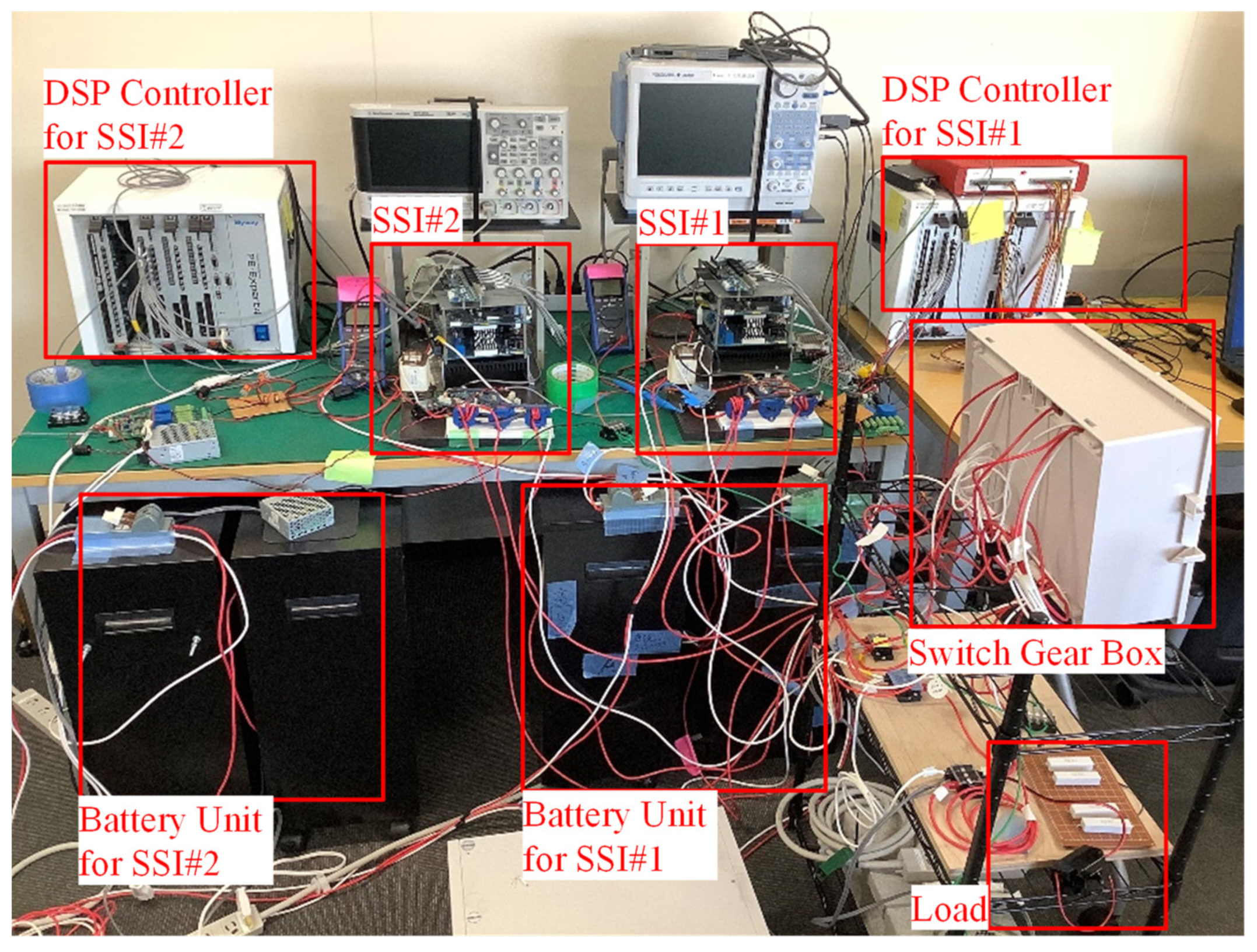
2.7. Hardware of the SSI
- DC voltage source: 16 lead-acid batteries (12 V) connected in series;
- Inductor: 10 mH/3.5 Apeak, Pony Electric, Gunma, Japan;
- Nosie Filter: NAH-20-472-B, COSEL, Toyama, Japan, is inserted at the output end to prevent noise on the power supply line;
- Current sensor: MWPE-IS-03, Myway Plus Corp, Yokohama, Japan;
- Voltage sensor: a self-made sensor circuit.
3. Development and Validation of the RMS Simulation Tool
3.1. Development of the RMS Simulation Tool Based on the NIC Design
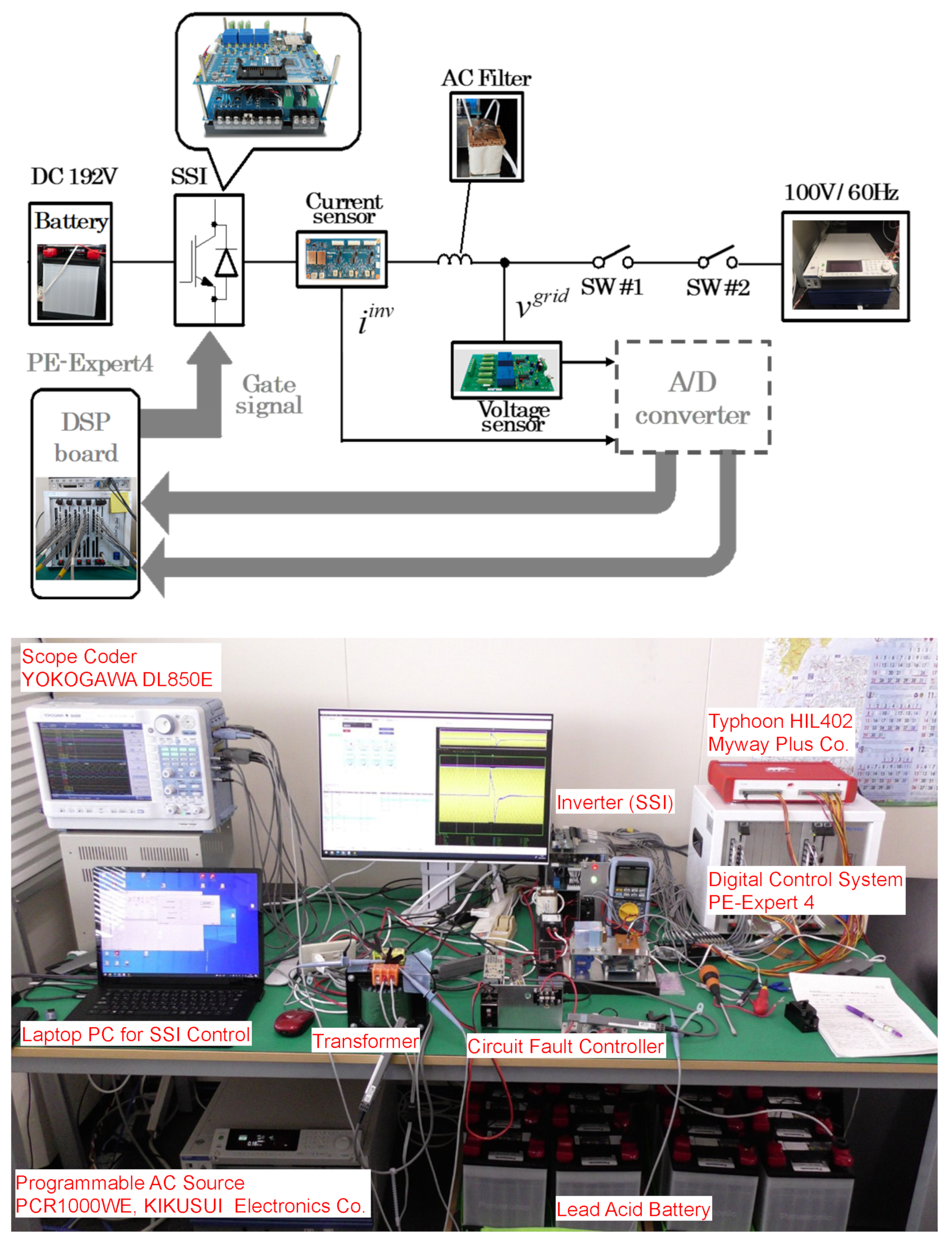
3.2. Experimental System of the Grid-Connected SSI for Validation
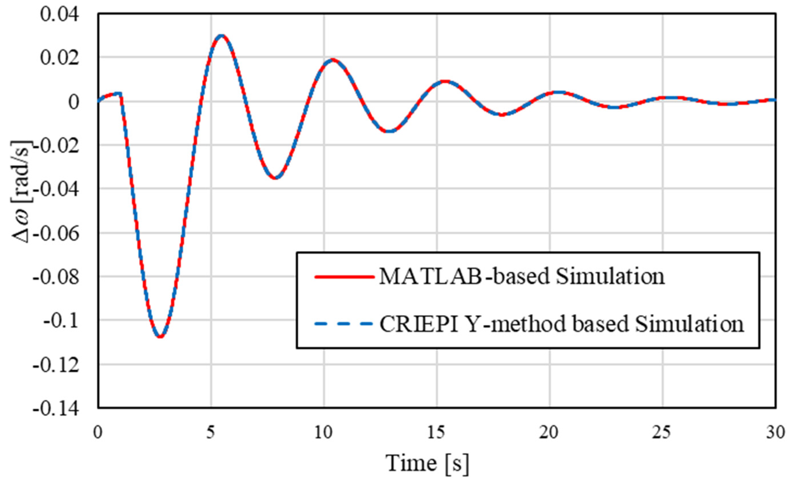
3.3. Comparison between Experiments, HIL, and RMS Simulations
4. Power System Stability Evaluation
4.1. Case Setting for Stability Assessment
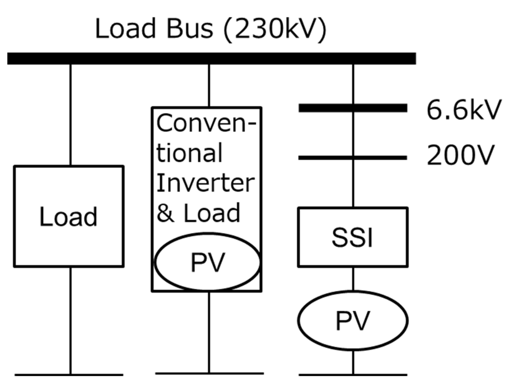
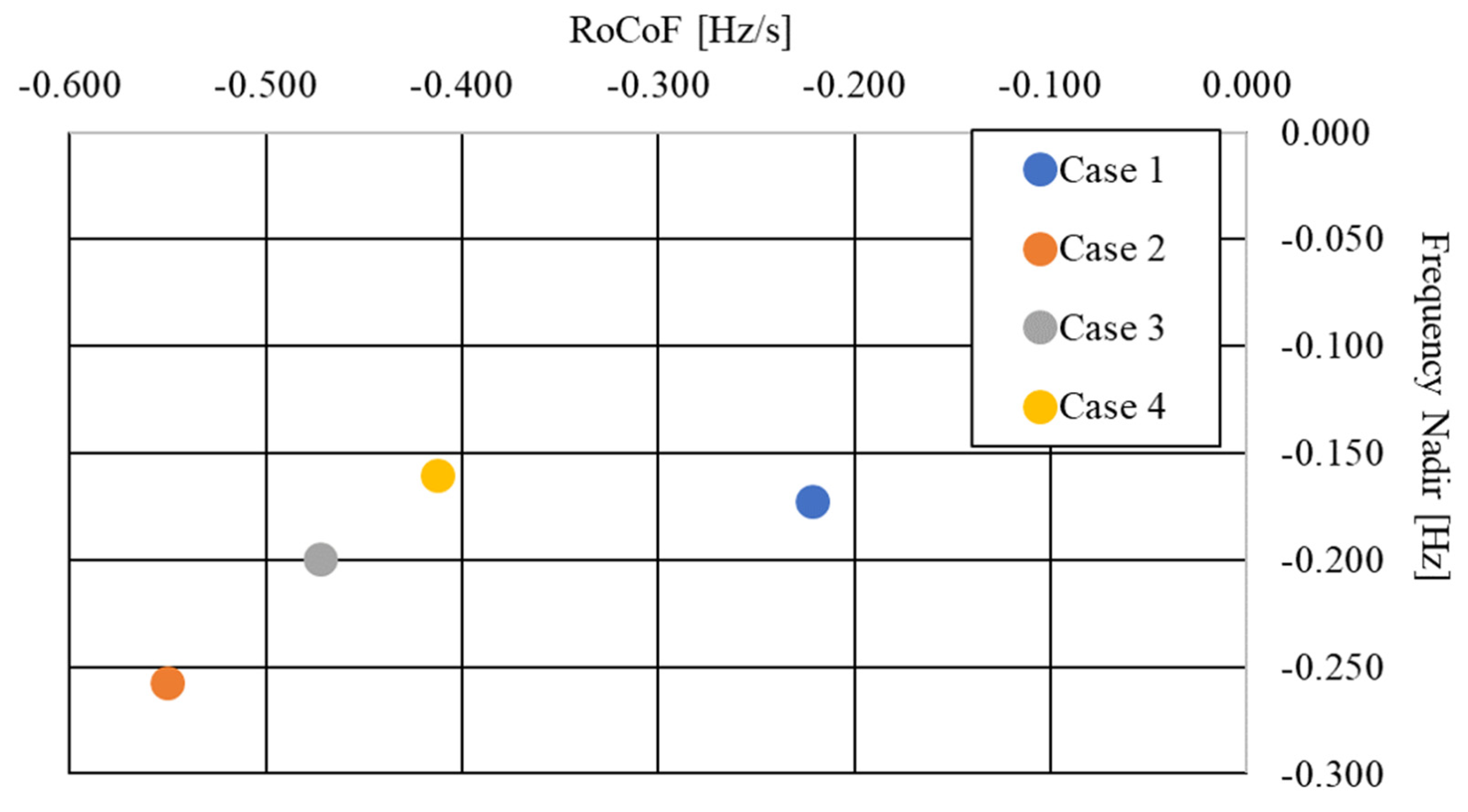
- Case 1: Represents the base condition of the test system in [40] where the total power is generated from the three conventional generators without any PV installations.
- Case 2: The PV penetration is 60% of the total power generation using conventional grid-following (GFL) inverters.
- Case 3: Half of the conventional GFL inverters of Case 2 are replaced by SSIs, which corresponds to about 80,000 SSIs of 1 kW.
- Case 4: All PV inverters are SSIs, about 160,000 SSIs.
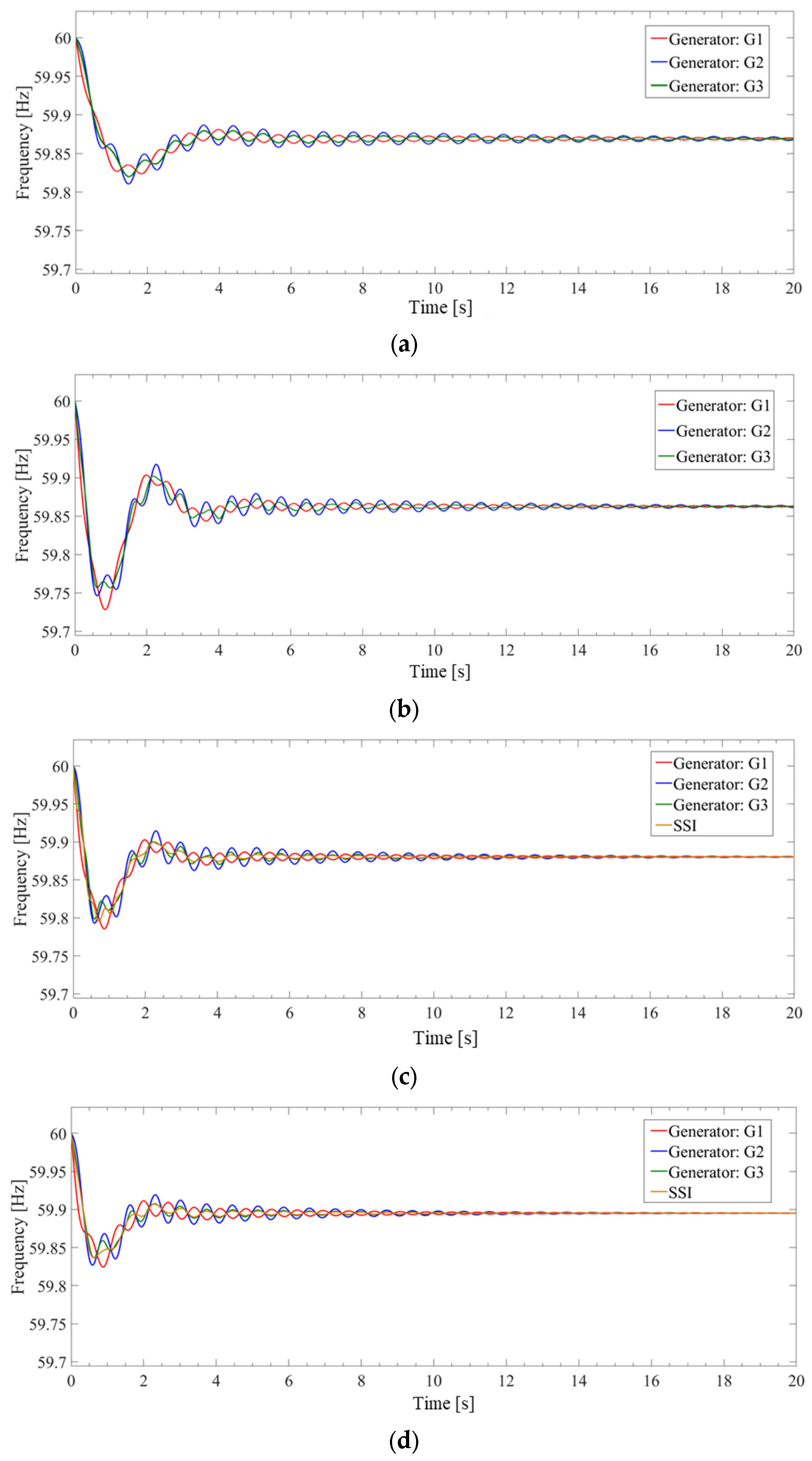
4.2. Frequency Stability Evaluation against Generator Trip
4.3. Transient Stability Evaluation for a Three-Phase Ground Fault
4.4. Small-Signal Stability Evaluation
5. Effective Design of the SMG Using the SSI
5.1. Design Concept of the SMG Using the NIC-SSI
5.2. Experimental Examinations of SMG Operations
5.2.1. Dynamic Performance of the SMG in Grid Connected (C0) and Stand-Alone (C1) Operations
| t = 0 [s]: |
|
| t = 15 [s]: |
|
| t = 25 [s]: |
|
| t = 40 [s]: |
|
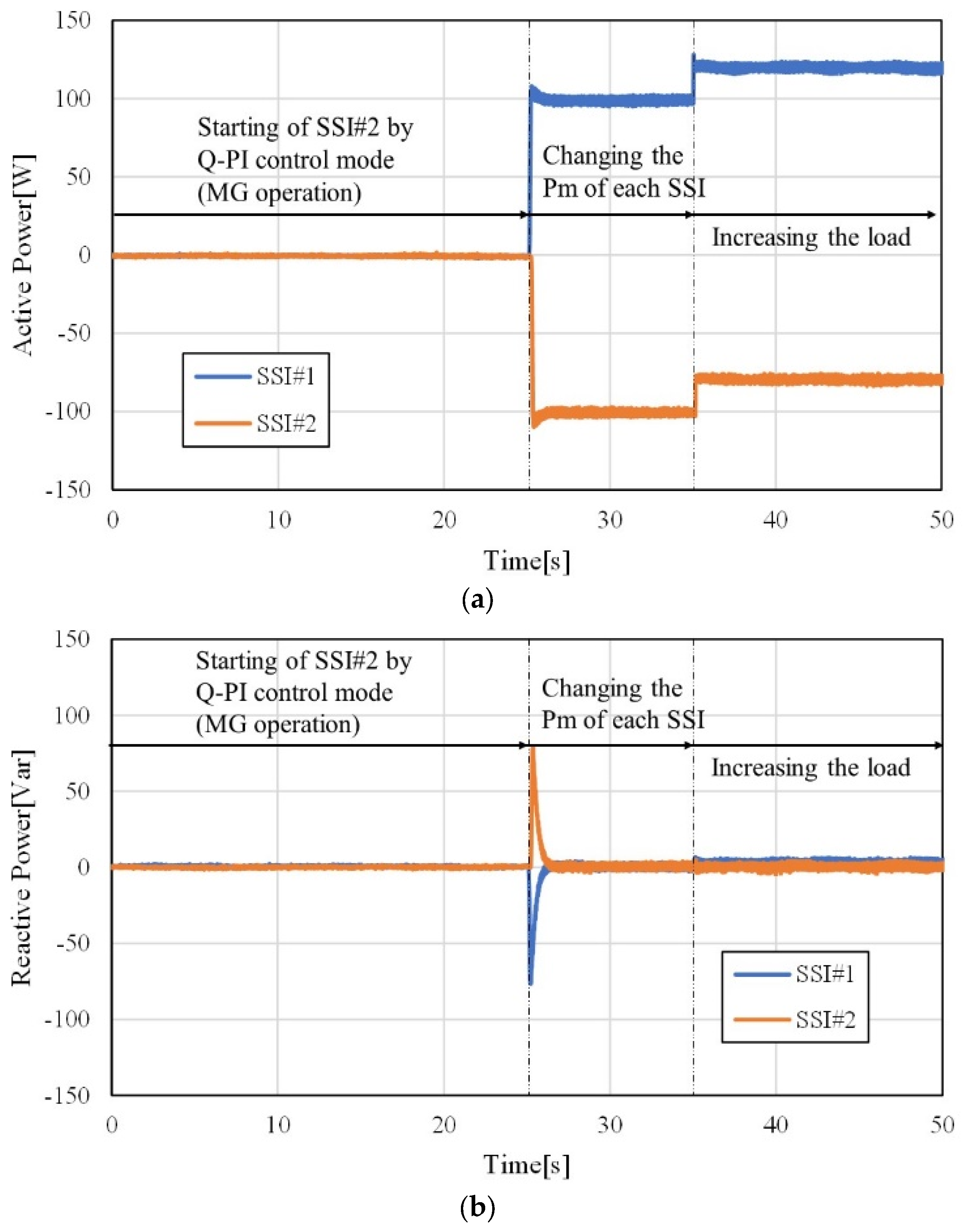
5.2.2. Dynamic Performance of the SMG in Stand-Alone (C1) to SMG (O2) Operations with Power Exchange between the SSIs
| t = 0 [s]: |
|
| t = 25 [s]: |
|
| t = 35 [s]: |
|
5.3. Experimental Examinations of SMG Operations with Ill-Conditioned Loads
5.3.1. SMG Operation Test Connected to a Grid-Simulated Power Supply
5.3.2. Off-Grid SMG Operation Test under Various Load Conditions
6. Conclusions
- An RMS simulation model was developed based on the NIC design method for stability analysis of a power system with SSIs as well as an SMG. The developed RMS model was accurate enough when compared with the experimental results. The error rate was about 10% for the maximum power swing (See Figure 10e, for example).
- Using the developed RMS analysis tool, the stabilization effects of the SSIs were investigated in the standard three-machine system. In the case where all PV inverters were replaced by SSIs on the demand side, considerable improvements were observed in terms of transient stability, small-signal stability, and frequency stability, where the frequency nadir was improved from −0.258 to −0.160, for example. (See Cases 2 and 4 in Table 7.)
- The performance of the SMG was demonstrated through experiments which show the feasibility and robust stability in terms of off-grid operations under various situations including ill-conditioned loads. (See the stable operation in Figure 32 for full-wave rectifier load.)
Author Contributions
Funding
Data Availability Statement
Conflicts of Interest
Abbreviations
| AC | Alternating Current |
| A/D | Analog-to-Digital Converter |
| AQR | Automatic Reactive Power Regulator |
| AVR | Automatic Voltage Regulator |
| CRIEPI | Central Research Institute of Electric Power Industry |
| DC | Direct Current |
| DSP | Digital Signal Processor |
| EMF | Electromotive Force |
| EMS | Energy Management System |
| FFR | Fast Frequency Response |
| GFL | Grid-Following |
| GFM | Grid-Forming |
| HIL | Hardware-In-the-Loop |
| HV | High-Voltage |
| IBR | Inverter-Based Resource |
| LV | Low-Voltage |
| MG | Microgrid |
| NEDO | New Energy and Industrial Technology Development Organization, National Research and Development Agency |
| NIC | Non-Interference Core |
| PI | Proportional Integration |
| PV | Photovoltaic Power Generation |
| Q-PI | Reactive Power Control with PI |
| RMS | Root Mean Square |
| RoCoF | Rate of Change of Frequency |
| SMG | Single-Phase Microgrid |
| SO-SOGI-QSG | Improved Second-Order–Second-Order Generalized Integrator based on Quadrature Signal Generation |
| SSI | Single-Phase Synchronous Inverter |
| THD | Total Harmonic Distortion |
| V-1L | Voltage Control with First-Order Delay |
| VRE | Variable Renewable Energy |
| VSCs | Voltage Source Converters |
| VSM | Virtual Synchronous Machine |
Appendix A


References
- Tayyebi, A.; Groß, D.; Anta, A.; Kupzog, F.; Dörfler, F. Frequency Stability of Synchronous Machines and Grid-Forming Power Converters. IEEE J. Emerg. Sel. Top. Power Electron. 2020, 8, 1004–1018. [Google Scholar] [CrossRef]
- Zhang, H.; Xiang, W.; Lin, W.; Wen, J. Grid Forming Converters in Renewable Energy Sources Dominated Power Grid: Control Strategy, Stability, Application, and Challenges. J. Mod. Power Syst. Clean Energy 2021, 9, 1239–1256. [Google Scholar] [CrossRef]
- Wang, X.; Taul, M.G.; Wu, H.; Liao, Y.; Blaabjerg, F.; Harnefors, L. Grid-Synchronization Stability of Converter-Based Resources—An Overview. IEEE Open J. Ind. Appl. 2020, 1, 115–134. [Google Scholar] [CrossRef]
- Laaksonen, H. Improvement of Power System Frequency Stability with Universal Grid-Forming Battery Energy Storages. IEEE Access 2023, 11, 10826–10841. [Google Scholar] [CrossRef]
- Milano, F.; Dorfler, F.; Hug, G.; Hill, D.J.; Verbič, G. Foundations and challenges of low-inertia systems (Invited Paper). In Proceedings of the 2018 Power Systems Computation Conference (PSCC), Dublin, Ireland, 11–15 June 2018. [Google Scholar] [CrossRef]
- Markovic, U.; Stanojev, O.; Aristidou, P.; Vrettos, E.; Callaway, D.; Hug, G. Understanding Small-Signal Stability of Low-Inertia Systems. IEEE Trans. Power Syst. 2021, 36, 3997–4017. [Google Scholar] [CrossRef]
- Paolone, M.; Gaunt, T.; Guillaud, X.; Liserre, M.; Meliopoulos, S.; Monti, A.; Van Cutsem, T.; Vittal, V.; Vournas, C. Fundamentals of power systems modelling in the presence of converter-interfaced generation. Electr. Power Syst. Res. 2020, 189, 106811. [Google Scholar] [CrossRef]
- Ahmed, F.; Kez, D.A.; McLoone, S.; Best, R.J.; Cameron, C.; Foley, A. Dynamic grid stability in low carbon power systems with minimum inertia. Renew. Energy 2023, 210, 486–506. [Google Scholar] [CrossRef]
- Kez, D.A.; Foley, A.; Ahmed, F.; Morrow, D.J. Overview of frequency control techniques in power systems with high inverter-based resources: Challenges and mitigation measures. IET Smart Grid 2023, 6, 447–469. [Google Scholar] [CrossRef]
- Li, L.; Zhu, D.; Zou, X.; Hu, J.; Kang, Y.; Guerrero, J.M. Review of frequency regulation requirements for wind power plants in international grid codes. Renew. Sustain. Energy Rev. 2023, 187, 113731. [Google Scholar] [CrossRef]
- Hong, Q.; Khan, M.A.U.; Henderson, C.; Egea-Àlvarez, A.; Tzelepis, D.; Booth, C. Addressing Frequency Control Challenges in Future Low-Inertia Power Systems: A Great Britain Perspective. Engineering 2021, 7, 1057–1063. [Google Scholar] [CrossRef]
- Su, L.; Qin, X.; Zhang, S.; Zhang, Y.; Jiang, Y.; Han, Y. Fast frequency response of inverter-based resources and its impact on system frequency characteristics. Glob. Energy Interconnect. 2020, 3, 475–485. [Google Scholar] [CrossRef]
- D’Arco, S.; Suul, J.A.; Fosso, O.B. A Virtual Synchronous Machine implementation for distributed control of power converters in SmartGrids. Electr. Power Syst. Res. 2015, 122, 180–197. [Google Scholar] [CrossRef]
- D’Arco, S.; Suul, J.A. Equivalence of virtual synchronous machines and frequency-droops for converter-based Microgrids. IEEE Trans. Smart Grid 2014, 5, 394–395. [Google Scholar] [CrossRef]
- Gunasekara, R.; Muthumuni, D.; Filizadeh, S.; Kho, D.; Marshall, B.; Ponnalagan, B.; Adeuyi, O.D. A Novel Virtual Synchronous Machine Implementation and Verification of Its Effectiveness to Mitigate Renewable Generation Connection Issues at Weak Transmission Grid Locations. IET Renew. Power Gener. 2022, 17, 2433–2678. [Google Scholar] [CrossRef]
- Zhong, Q.C.; Weiss, G. Synchronverters: Inverters that mimic synchronous generators. IEEE Trans. Ind. Electron. 2011, 58, 1259–1267. [Google Scholar] [CrossRef]
- Kryonidis, G.C.; Malamaki, K.N.D.; Mauricio, J.M.; Demoulias, C.S. A New Perspective on the Synchronverter Model. Int. J. Electr. Power Energy Syst. 2022, 140, 108072. [Google Scholar] [CrossRef]
- Zhang, L.; Harnefors, L.; Nee, H.P. Power-synchronization control of grid-connected voltage-source converters. IEEE Trans. Power Syst. 2010, 25, 809–820. [Google Scholar] [CrossRef]
- Alawasa, K.M.; Mohamed, Y.A.R.I. Impedance and damping characteristics of grid-connected VSCs with power synchronization control strategy. IEEE Trans. Power Syst. 2015, 30, 952–961. [Google Scholar] [CrossRef]
- Tayab, U.B.; Roslan, M.A.B.; Hwai, L.J.; Kashif, M. A review of droop control techniques for microgrid. Renew. Sustain. Energy Rev. 2017, 76, 717–727. [Google Scholar] [CrossRef]
- Sekizaki, S.; Nakamura, Y.; Sasaki, Y.; Yorino, N.; Zoka, Y.; Nishizaki, I. A development of pseudo-synchronizing power VSCs controller for grid stabilization. In Proceedings of the 2016 Power Systems Computation Conference (PSCC), Genoa, Italy, 20–24 June 2016. [Google Scholar] [CrossRef]
- Sekizaki, S.; Yorino, N.; Sasaki, Y.; Matsuo, K.; Nakamura, Y.; Zoka, Y.; Shimizu, T.; Nishizaki, I. Proposal of a single-phase synchronous inverter with noninterference performance for power system stability enhancement and emergent microgrid operation. Electr. Eng. Jpn. 2019, 207, 3–13, Original paper: IEEJ Trans. Power Energy 2018, 138, 893–901. [Google Scholar] [CrossRef]
- EU Project POSYTYF—Powering System Flexibility in the Future Renewable Energy Sources, On-Going as of 2023. Available online: https://posytyf-h2020.eu/ (accessed on 8 January 2024).
- US Project Unifi (Universal Interoperability for Grid-Forming Inverters)—Unifing Inverters and Grids, On-Going as of 2023. Available online: https://sites.google.com/view/unifi-consortium/home (accessed on 8 January 2024).
- Australia ARENA Project Broken Hill Battery Energy Storage System, On-Going as of 2023. Available online: https://arena.gov.au/projects/agl-broken-hill-grid-forming-battery/ (accessed on 8 January 2024).
- Marinescu, S.; Gomis-Bellmunt, O.; Dörfler, F.; Schulte, H.; Sigrist, L. Dynamic Virtual Power Plant: A New Concept for Grid Integration of Renewable Energy Sources. IEEE Access 2022, 10, 104980–104995. [Google Scholar] [CrossRef]
- Collados-Rodriguez, C.; Spier, W.D.; Cheah-Mane, M.; Prieto-Araujo, E.; Gomis-Bellmunt, O. Preventing loss of synchronism of droop-based grid-forming converters during frequency excursions. Int. J. Electr. Power Energy Syst. 2023, 148, 108989. [Google Scholar] [CrossRef]
- Collados-Rodríguez, C.; Antolí-Gil, E.; Sánchez-Sánchez, E.; Girona-Badia, J.; Lacerda, V.A.; Cheah-Mañe, M.; Prieto-Araujo, E.; Gomis-Bellmunt, O. Definition of Scenarios for Modern Power Systems with a High Renewable Energy Share. Glob. Chall. 2023, 7, 2200129. [Google Scholar] [CrossRef] [PubMed]
- Lacerda, V.A.; Araujo, E.P.; Chea-Mañe, M.; Gomis-Bellmunt, O. Phasor and EMT models of grid-following and grid-forming converters for short-circuit simulations. Electr. Power Syst. Res. 2023, 223, 109662. [Google Scholar] [CrossRef]
- Liu, Y.; Huang, R.; Du, W.; Singhal, A.; Huang, Z. Highly-Scalable Transmission and Distribution Dynamic Co-Simulation with 10,000+ Grid-Following and Grid-Forming Inverters. IEEE Trans. Power Deliv. 2023, 1–12, Early Access. [Google Scholar] [CrossRef]
- Lu, M.; Cai, W.; Dhople, S.; Johnson, B. Large-signal Stability of Phase-balanced Equilibria in Single-phase Grid-forming Inverter Systems. IEEE Trans. Power Electron. 2023, 1–14, Early Access. [Google Scholar] [CrossRef]
- Islam, M.D.; Muttaqi, K.M.; Sutanto, D.; Rahman, M.M.; Alonso, O. Design of a Controller for Grid Forming Inverter-Based Power Generation Systems. IEEE Access 2023, 11, 2169–3536. [Google Scholar] [CrossRef]
- Areed, E.F.; Yan, R.; Saha, T.K. Impact of Battery Ramp Rate Limit on Virtual Synchronous Machine Stability During Frequency Events. IEEE Trans. Sustain. Energy 2024, 15, 567–580. [Google Scholar] [CrossRef]
- Yorino, N.; Sekizaki, S.; Adachi, K.; Sasaki, Y.; Zoka, Y.; Bedawy, A.; Shimizu, T.; Amimoto, K. A Novel Design of Single-phase Microgrid Based on Non-Interference Core Synchronous Inverters for Power System Stabilization. IET Gener. Transm. Distrib. 2022, 17, 2861–2875. [Google Scholar] [CrossRef]
- Farrokhabadi, M.; Canizares, C.A.; Simpson-Porco, J.W.; Nasr, E.; Fan, L.; Mendoza-Araya, P.A.; Tonkoski, R.; Tamrakar, U.; Hatziargyriou, N.; Lagos, D.; et al. Microgrid Stability Definitions, Analysis, and Examples. IEEE Trans. Power Syst. 2020, 35, 3513–3529. [Google Scholar] [CrossRef]
- Sekizaki, S.; Matsuo, K.; Sasaki, Y.; Yorino, N.; Nakamura, Y.; Zoka, Y.; Shimizu, T.; Nishizaki, I. A Development of Single-phase Synchronous Inverter and Integration to Single-phase Microgrid effective for frequency stability enhancement. IFAC-Pap. OnLine 2018, 51, 245–250. [Google Scholar] [CrossRef]
- Yorino, N.; Sasaki, H.; Masuda, Y.; Tamura, Y.; Kitagawa, M.; Oshimo, A. An investigation of voltage instability problems. IEEE Trans. Power Syst. 1992, 7, 600–611. [Google Scholar] [CrossRef]
- Sekizaki, S.; Yorino, N.; Sasaki, Y.; Zoka, Y.; Shimizu, T.; Nishizaki, I. Single-phase Synchronous Inverter with Overcurrent Protection using Current Controller with Latched Limit Strategy. IEE J. Trans. Electr. Electron. Eng. 2021, 18, 1001–1014. [Google Scholar] [CrossRef]
- Xin, Z.; Wang, X.; Qin, Z.; Lu, M.; Loh, P.C.; Blaabjerg, F. An Improved Second-Order Generalized Integrator Based Quadrature Signal Generator. IEEE Trans. Power Electron. 2016, 31, 8068–8073. [Google Scholar] [CrossRef]
- Anderson, P.M.; Fouad, A.A. Power System Control and Stability, 2nd ed.; Wiley—IEEE Press: Hoboken, NJ, USA, 2003. [Google Scholar]
- KAKEN—Research Projects | Construction of a Single-Phase Microgrid Using an Actual Machine (KAKENHI-PROJECT-20H00251). Available online: https://kaken.nii.ac.jp/en/grant/KAKENHI-PROJECT-20H00251/ (accessed on 22 October 2021).


| Parameters | Values |
|---|---|
| Rfil | 0.48 Ω |
| Lfil | 10 mH |
| Lnf | 1.4 mH |
| Rnf | 470 kΩ |
| Cnf | 0.95 μF |
| Rfault | 100/3 Ω |
| Rt1 | 1.00 Ω |
| Lt1 | 1.48 mH |
| Rt2 | 43.4 Ω |
| Lt2 | 516.1 mH |
| Parameters | Values |
|---|---|
| [W·s2/rad] | 1 * |
| Pm [W] | 0 |
| ωref [rad/s] | 120π |
| (Simulink, HIL) [W∙s/rad] | 100 |
| (Experimental) [W∙s/rad] | 50 * |
| Vref [V] | 100 |
| Qref [var] | 0 |
| Qsig (“0”: AVR, “1”: AQR) | 1 |
| SW condition (“0” = 1 L, “1” = PI) | 1 |
| Ka | 1 |
| Kp | 0 |
| Ki | 5 |
| KQ | 0.05 |
| Fault Timing | Fault Duration Time | Pe [W] (Maximum RMS) | |
|---|---|---|---|
| [°] | [s] | ||
| 0 | 0.4160 | 0.0160 | 50.51 |
| 10 | 0.4158 | 0.0158 | 52.73 |
| 20 | 0.4153 | 0.0153 | 52.61 |
| 30 | 0.4147 | 0.0147 | 50.40 |
| 40 | 0.4142 | 0.0142 | 49.65 |
| 50 | 0.4136 | 0.0136 | 48.08 |
| 60 | 0.4133 | 0.0133 | 50.79 |
| 70 | 0.4123 | 0.0123 | 45.30 |
| 80 | 0.4205 | 0.0205 | 45.97 |
| 90 | 0.4201 | 0.0201 | 47.06 |
| 100 | 0.4197 | 0.0197 | 48.74 |
| 110 | 0.4194 | 0.0194 | 50.24 |
| 120 | 0.4189 | 0.0189 | 50.08 |
| 130 | 0.4186 | 0.0186 | 51.69 |
| 140 | 0.4179 | 0.0179 | 52.02 |
| 150 | 0.4177 | 0.0177 | 52.68 |
| 160 | 0.4173 | 0.0173 | 53.06 |
| 170 | 0.4167 | 0.0167 | 53.70 |
| 180 | 0.4161 | 0.0161 | 51.93 |
| Disturbance | Stability | Evaluation Indices |
|---|---|---|
| Generator Outage | Frequency Stability Small-Signal Stability | RoCoF, Frequency Nadir Eigenvalues |
| Three-Phase Ground Fault | Transient Stability Small-Signal Stability | Generator Swings Eigenvalues |
| Case | Total Generator’ Output [%] | Total PV Output [%] | |
|---|---|---|---|
| (G1 + G2 + G3) | Conventional Inverters | Proposed SSIs | |
| Case 1 | 100 | 0 | 0 |
| Case 2 | 40 | 60 | 0 |
| Case 3 | 30 | 30 | |
| Case 4 | 0 | 60 | |
| Parameters | Generators and SSI | |||
|---|---|---|---|---|
| G1 | G2 | G3 | SSI(/Machine) | |
| Rated Capacity | 247.5 [MVA] | 192.0 [MVA] | 128.0 [MVA] | 1 [kVA] |
| H [s] | 23.64 | 6.4 | 3.01 | 9.42 |
| D [p.u.] | 2.0 | 2.0 | 2.0 | 37.7 |
| xd′ [p.u.] | 0.0608 | 0.1198 | 0.1813 | 0.4298 |
| KGOV | 0.0663 | 0.0663 | 0.0663 | 0.1 |
| TGOV [s] | 1.0 | 0.5 | 0.5 | 0.02 |
| KAVR [s] | 0.1 | 0.1 | 0.1 | 0.1 |
| TAVR [s] | 0.5 | 0.5 | 0.5 | 0.5 |
| Cases | Nadir [Hz] | RoCoF [Hz/s] |
|---|---|---|
| Case 1 | −0.173 | −0.222 |
| Case 2 | −0.258 | −0.551 |
| Case 3 | −0.199 | −0.472 |
| Case 4 | −0.160 | −0.413 |
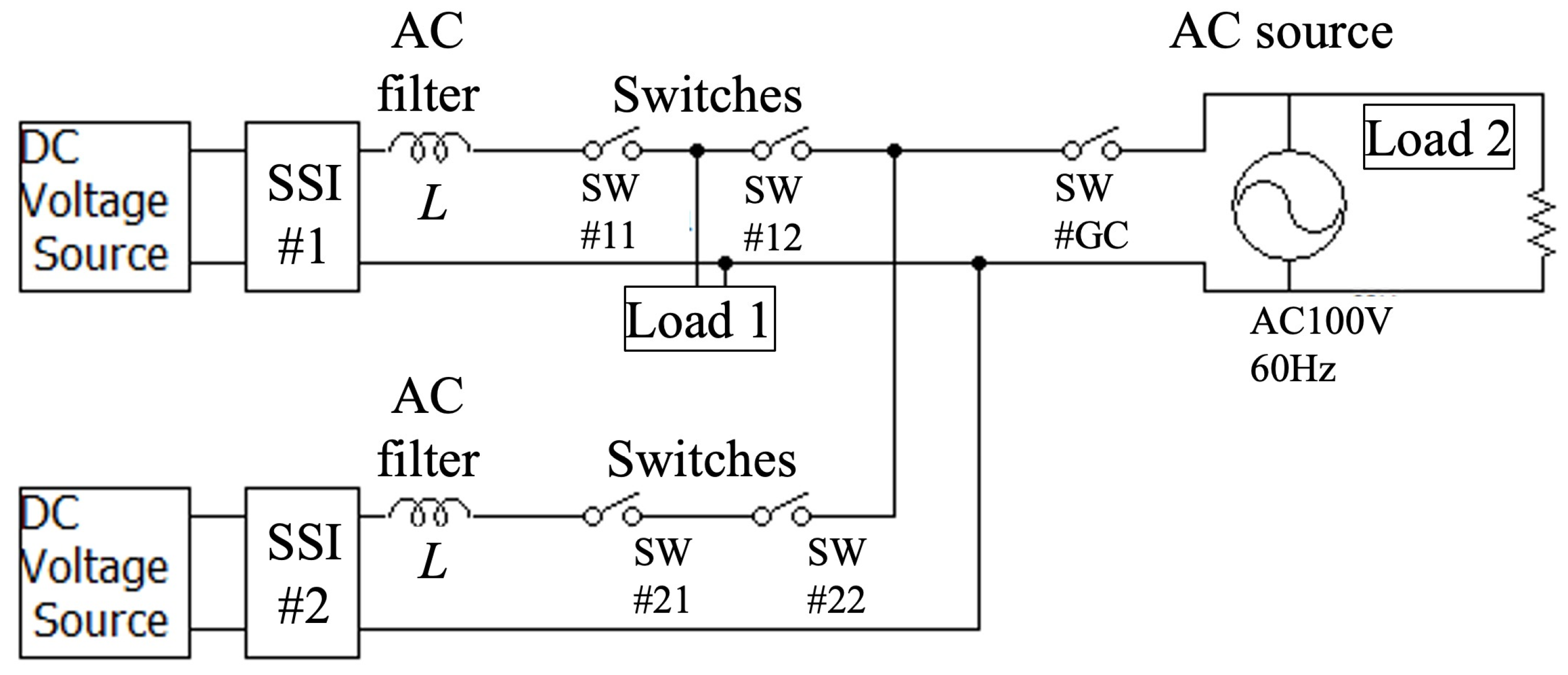
| Operation Mode | SW #11 | SW #21 | SW #12 | SW #22 | SW #GC | Control Mode | |
|---|---|---|---|---|---|---|---|
| Case C0 | In a normal state | × | × | ○ | ○ | ○ | |
| Case O0 | In a power outage | × | × | ○ | ○ | × | |
| Case C1 | SSI#1 grid-connected operation | ○ | × | ○ | ○ | ○ | SSI#1: Q-PI |
| Case O1 | SSI#1 stand-alone operation | ○ | × | ○ | ○ | × | SSI#1: V-1L |
| Case O2 | SSI#1 off-grid operation | ○ | ○ | ○ | ○ | × | SSI#1: V-1L SSI#2: Q-PI |
| Parameters | Values |
|---|---|
| AC filter L | 10 mH |
| Load 1 | Light (AC100 V, 100 W) for the resistive load connection test |
| Light (AC100 V, 20 W) for the lag load connection test and distortion load connection test | |
| Load 2 | Transformer (T-200, 2.1 kVA, Yamabishi, Tokyo, Japan) for the lag load connection test |
| Switching regulator (PR18-3A, KENWOOD, Tokyo, Japan) for the lag load connection test | |
| Variable resistance (D-8, Yamabishi) for the lag load connection test |
| (1) Grid-connection Test | No-load, depending on system voltage |
| (2) Resistive Load Connection Test | System Voltage: V = 98.2 V, THD = 0.35% SSI#1: I1 = 0.49A, THD1 = 1.53% SSI#2: I2 = 0.49A, THD2 = 0.00% |
| (3) Lag Load Connection Test | System Voltage: V = 97.2 V, THD = 1.44% SSI#1: I1 = 0.59A, THD1 = 16.66%, P.F. = 0.796 SSI#2: I2 = 0.59A, THD2 = 16.45% |
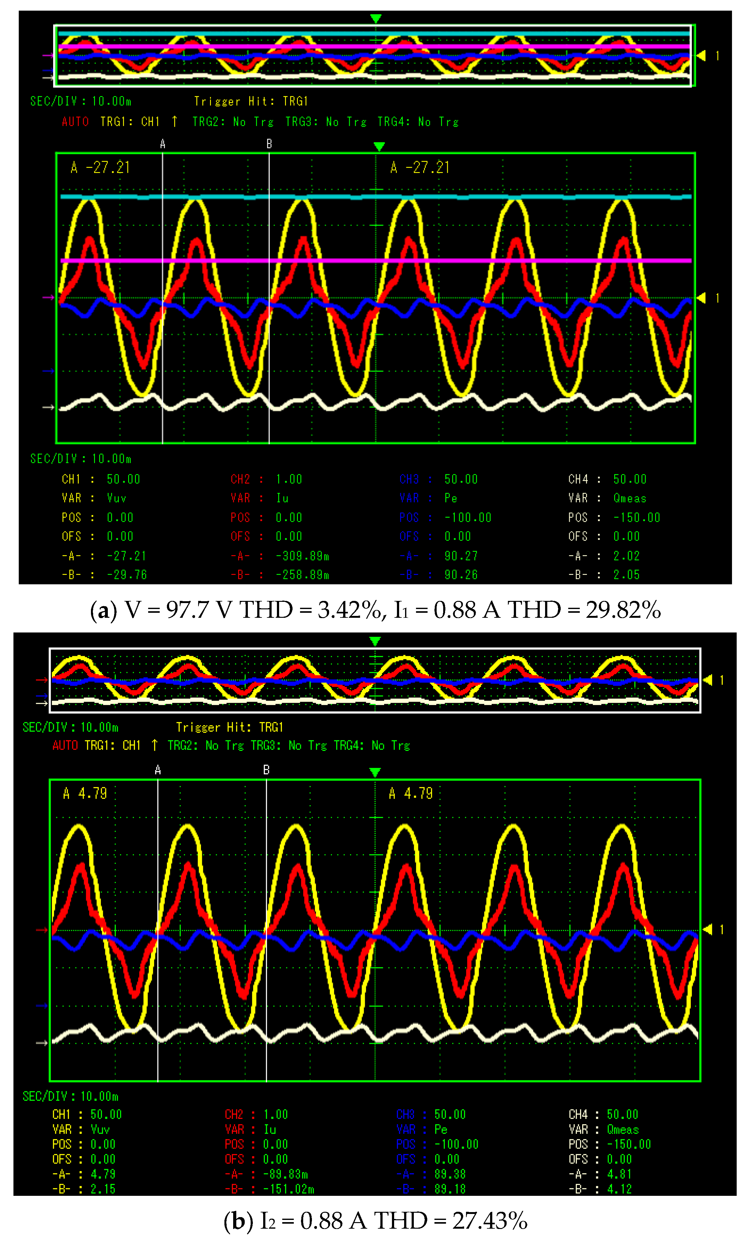
| (4) Distortion LoadConnection Test | System Voltage: V = 97.7 V, THD = 3.42% SSI#1: I1 = 0.88A, THD1 = 29.82% SSI#2: I2 = 0.88A, THD2 = 27.43% |
Disclaimer/Publisher’s Note: The statements, opinions and data contained in all publications are solely those of the individual author(s) and contributor(s) and not of MDPI and/or the editor(s). MDPI and/or the editor(s) disclaim responsibility for any injury to people or property resulting from any ideas, methods, instructions or products referred to in the content. |
© 2024 by the authors. Licensee MDPI, Basel, Switzerland. This article is an open access article distributed under the terms and conditions of the Creative Commons Attribution (CC BY) license (https://creativecommons.org/licenses/by/4.0/).
Share and Cite
Yorino, N.; Zoka, Y.; Sasaki, Y.; Sekizaki, S.; Yokonuma, M.; Himuro, T.; Kuroki, F.; Fujii, T.; Inoue, H. Development of Single-Phase Synchronous Inverter for Single-Phase Microgrid. Electronics 2024, 13, 478. https://doi.org/10.3390/electronics13030478
Yorino N, Zoka Y, Sasaki Y, Sekizaki S, Yokonuma M, Himuro T, Kuroki F, Fujii T, Inoue H. Development of Single-Phase Synchronous Inverter for Single-Phase Microgrid. Electronics. 2024; 13(3):478. https://doi.org/10.3390/electronics13030478
Chicago/Turabian StyleYorino, Naoto, Yoshifumi Zoka, Yutaka Sasaki, Shinya Sekizaki, Mitsuo Yokonuma, Takahiro Himuro, Futoshi Kuroki, Toshinori Fujii, and Hirotaka Inoue. 2024. "Development of Single-Phase Synchronous Inverter for Single-Phase Microgrid" Electronics 13, no. 3: 478. https://doi.org/10.3390/electronics13030478