Article

A Method for Visualization of Images by Photon-Counting Imaging Only Object Locations under Photon-Starved Conditions

1
Department of Computer Science and Networks, Kyushu Institute of Technology, 680-4 Kawazu, Iizuka-shi 820-8502, Fukuoka, Japan
2
School of ICT, Robotics, and Mechanical Engineering, Hankyong National University, IITC, 327 Chungang-ro, Anseong 17579, Kyonggi-do, Republic of Korea
*
Authors to whom correspondence should be addressed.
These authors contributed equally to this work.
Electronics 2024, 13(1), 38; https://doi.org/10.3390/electronics13010038
Submission received: 13 November 2023 / Revised: 11 December 2023 / Accepted: 18 December 2023 / Published: 20 December 2023

Abstract

:
Recently, many researchers have been studying the visualization of images and the recognition of objects by estimating photons under photon-starved conditions. Conventional photon-counting imaging techniques estimate photons by way of a statistical method using Poisson distribution in all image areas. However, Poisson distribution is temporally and spatially independent, and the reconstructed image has a random noise in the background. Random noise in the background may degrade the quality of the image and make it difficult to accurately recognize objects. Therefore, in this paper, we apply photon-counting imaging technology only to the area where the object is located to eliminate the noise in the background. As a result, it can be seen that the image quality using the proposed method is better than that of the conventional method and the object recognition rate is also higher. Optical experiments were conducted to prove the denoising performance of the proposed method. In addition, we used the structure similarity index measure (SSIM) as a performance metric. To check the recognition rate of the object, we applied the YOLOv5 model. Finally, the proposed method is expected to accelerate the development of astrophotography and medical imaging technologies.

1. Introduction

Recently, research on estimating and visualizing photons under photon-starved conditions has been conducted in various fields such as aerospace optics, medical optics, etc. Furthermore, there is a new field of research using photon-counting detectors (PCDs), which detect photon energy to visualize images [1,2,3,4,5,6,7,8,9,10,11,12,13,14,15,16,17,18,19]. The Hubble Space Telescope (HST), launched from Earth in 1990, is a space telescope developed by the National Aeronautics and Space Administration (NASA) and the European Space Agency (ESA) that is used for observational astronomy from space [2]. The HST is equipped with a variety of cameras, spectrographs, and optical instruments, including a spectrograph optimized for ultraviolet observation, which uses PCDs with photon-counting technology that perform better than a CCD (Charge-Coupled Device) at estimating and visualizing ultraviolet photons even under photon-starved conditions such as in space [2,3,4,5]. As a result, the HST has enabled the observation of the expanding universe as well as the Hubble constant measurement project, which has provided us with a deeper understanding of the universe and its structure [6,7].
Hounsfield was awarded the 1979 Nobel Prize in Physiology or Medicine for developing and first introducing the medical imaging technology computed tomography (CT) into medicine [8,9]. X-ray CT is a medical imaging technique that non-destructively reconstructs three-dimensional (3D) images of human internal structures. More recently, advances in X-ray CT imaging technology have led to the development of photon-counting computed tomography (PCCT), which uses PCDs to estimate individual incoming X-ray photons and measure their energy levels [10,11,12]. PCDs can significantly reduce image noise and increase spatial resolution, and k-edge imaging can be used to measure the concentration of specific elements for material discrimination. Moreover, these technological advances will reduce radiation dose by at least 30–40% compared to traditional X-ray CT imaging techniques [10]. Techniques, such as using PCDs to estimate individual incoming X-ray photons and measure their energy levels, have been developed by many researchers in recent years [2,3,4,5,6,7,8,9,10,11,12,13,14]. However, PCDs may have some imperfections. First, charge sharing occurs when an X-ray photon arrives near the boundary between two pixels. This causes the X-ray photon to be detected both times at the wrong energy, reducing spatial resolution. Second, two independent photons may arrive at the same pixel at very high speeds, causing the signal to “pile up” and be interpreted by the electronic processing unit as a single photon. Finally, PCDs can be susceptible to electron noise, similar to CCDs, and suffer from the problem that measurements become uncertain when low-energy photons are detected [15]. Many researchers have studied these problems [20], and research is ongoing to accurately estimate photons to visualize images.
In general, photon-counting imaging techniques use a specialized sensor such as an EM-CCD camera, rather than a general camera, to acquire images. However, these specialized sensors require high prices and are difficult to commercialize. To overcome this problem, in this paper, we use a computational algorithm with a general camera to implement a photon-counting imaging technique [18,21,22,23,24,25,26]. Photon-counting imaging techniques, which estimate photons in a statistical way, may be an alternative to the conventional PCD problem. The computational photon-counting imaging method is an image processing technique that solves the hardware problems of photon-counting imaging by using software methods similar to the physical photon-counting imaging method. Photon-counting imaging techniques can visualize images by estimating photons that rarely occur in a unit of time and space based on Poisson distribution [16,17,18,19,21,22,23,24,25,26]. However, it also has a problem of random noise, and photons can be detected from objects as well as from the background, which degrade the visual quality of the image. Several studies have applied filters to remove the random noise in this background, most notably the median filter or the Kalman filter [21,22]. Using these filters can reduce the quality of the image because they remove not only background noise, but also information about the object. To solve these problems, in this paper, we propose a novel photon-counting imaging method to classify object location and the number of photons by section (COLaNoPS). Since the conventional photon-counting imaging technique applies a Poisson random process to all of the image, we can recognize the random noise from both the object and the background. Therefore, we need to remove noise from the background by applying Poisson distribution only to the area where the object exists. To estimate the location of an object, we assume that the photon energy at the location of the object is higher than that of the background. A threshold for the presence of an object is defined by measuring the photon energy as a section of a certain size moves throughout it. This algorithm reduces noise in the background by applying Poisson distribution only to the area in which the object is present, based on the threshold. As the section moves throughout the image, it applies spatial overlap to the area where the photons overlap each other to improve the photon energy of the object. As a result, we can estimate the photon energy of the object, improving the visual quality of the image.
This paper is organized as follows. In Section 2, we describe conventional photon-counting imaging techniques and the proposed method that estimates the photon energy of the object to reduce background noise. Then, we perform the optical experiment and show the results in Section 3. Finally, in Section 4, we present our conclusions and future works.

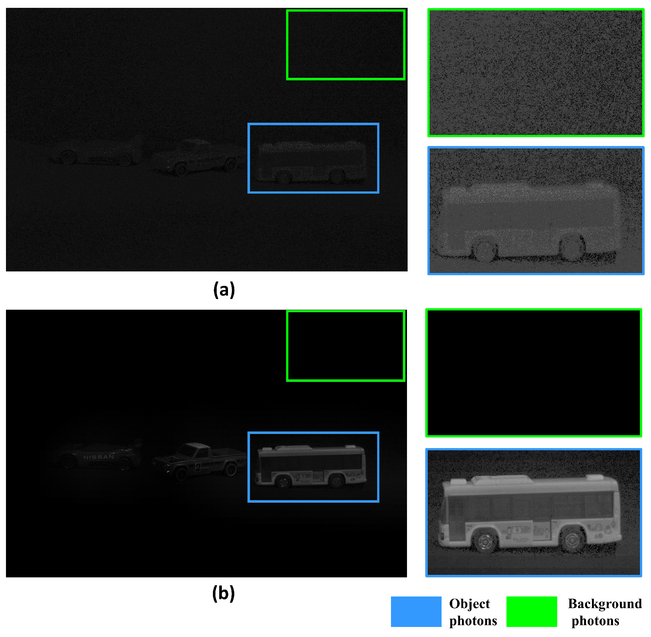
2. Reducing Background Noise by Estimating Photons Only in the Object Area

2.1. Photon-Counting Imaging

The human eye can see objects by converting the properties of light reflected from them into electrical signals through the rod and cone cells of the retinal cells. The image sensor (CCD or complementary metal-oxide semiconductor (CMOS) sensor) in the camera is a device similar to the human eye, which uses the photoelectric effect to detect the nature of reflected light and can visualize objects. Therefore, the image sensor in the camera suffers from the inability to visualize objects under photon-starved conditions. To solve this problem, photon-counting imaging techniques [16,17,18,19,21,22,23] can be one of the alternatives to visualizing images under photon-starved conditions. Photon-counting imaging technology estimates photons for an object by applying a statistical process of Poisson distribution to each image pixel under photon-starved conditions. Furthermore, the accuracy of the estimated photons can be improved by applying the maximum likelihood estimation (MLE) and a Bayesian approach such as the maximum a posteriori (MAP). MLE and MAP are the main methods for solving the classification problems using probability. MLE is the method of selecting the class with the maximum likelihood, and MAP is the method of selecting the class with the maximum posterior probability [16,19]. We apply a Poisson distribution to probabilistically estimate the photons of an object under photon-starved conditions. We apply MLE and MAP to the estimated photons for solving the classification problem of determining whether a photon occurs or not. Since photons rarely occur in unit time and space under photon-starved conditions, we can assume that they follow a Poisson distribution, and the Poisson distribution is defined by the following equations:
λ E ( x , y ) = I E ( x , y ) x = 1 N x y = 1 N y I E ( x , y )
C E x , y N p λ E ( x , y ) P o i s s o n N p λ E x , y ,
where λ E ( x , y ) is the normalized intensity of the image at position ( x , y ) of each elemental image in the array, I E is the intensity of the elemental image, N x and N y are the total number of image pixels, and x and y are the pixel positions of each elemental image, respectively. In addition, C E is the estimated photons in the elemental image, and N p is the expected number of photons for each elemental image. The likelihood function and log-likelihood function of the λ E normalized elemental images are defined as follows [16,17,18,19,21,22,23]:
P C k l | N p λ k l = k = 0 k 1 l = 0 L 1 e N p λ k l ( N p λ k l ) C k l C k l ! ,
L N p λ k l | C k l k = 0 K 1 l = 0 L 1 C k l l o g N p λ k l k = 0 K 1 l = 0 L 1 N p λ k l ,
where λ k l is assumed to be a matrix of k rows and l columns all extracted independently from the elemental images. P ( C k l | N p λ k l ) is the likelihood function, L ( N p λ k l | C k l ) is the log-likelihood function. The MLE for estimating by maximizing the likelihood function is defined as follows:
L N p λ k l | C k l λ k l = C k l λ k l N p = 0 ,
λ k l M L E = C k l N p .
In Equations (5) and (6), we can define the MLE for the normalized elemental image λ k l as λ k l M L E by taking a partial derivative of L ( N p λ k l | C k l ) to λ k l . As a result, we can derive the MLE of each elemental image as shown in Figure 1 [16,17,18].
Figure 1 shows the process of the photon-counting imaging by MLE. However, in MLE, the estimation accuracy may be low because it uses uniform distribution as the prior information, which means that the occurrence of photons for each pixel has the same probability. Therefore, more specific prior information is required to obtain better estimation accuracy. A Bayesian approach such as MAP uses the specific statistical distribution as the prior information. In this paper, we assume that the normalized elemental image with the expected number of photons N p λ k l follows a Gamma ( Γ ) distribution because a general image has a [0 255] pixel range. The MAP method uses the statistical parameters α and β of the image’s prior probability distribution, which is defined as a Γ distribution. To estimate λ k l , a posterior distribution is calculated and maximized by multiplying the likelihood function for each elemental image using prior information [19,21,22,23].
π N p λ k l = β α Γ α ( N p λ k l ) α 1 e β N p λ k l , N p λ k l > 0
μ = α β , σ 2 = α β 2 α 2 = μ 2 σ 2 , β = μ σ 2 ,
π N p λ k l | C k l G a m m a C k l + α , 1 + β ,
where π ( N p λ k l ) is a Γ distribution of the normalized elemental image with the expected number of photons, which is a prior probability distribution and a conjugate prior of Poisson distribution; α and β are the statistical parameters of the Γ distribution and they are both positive; μ , σ 2 are the mean and variance of N p λ k l ; π ( N p λ k l | C k l ) is modeled as a conjugate family of distributions for ease of calculating the G a m m a distribution, respectively [22,23].
λ k l M A P = C k l + α N p 1 + β , C k l > 0 .
By using Equations (7)–(9), we can calculate the posterior distribution and the estimator of elemental images as written in Equation (10). The original image is reconstructed using the mean of the posterior distribution from each elemental image. That is, λ k l M A P can be defined as the mean of a posterior distribution by MAP [23].
Figure 2 shows the reconstructed images by MLE and MAP under photon-starved conditions. The MAP method can reconstruct the image by estimating the photons more accurately than the MLE method under these conditions with the same number of photons.
Figure 3 shows a noisy image from the background when the image is reconstructed by estimating photons with MAP. To visualize the noise, we increased the brightness by 40% and decreased the contrast by 40%. As shown in Figure 3, the MAP method can estimate photons more accurately than the MLE method to visualize the image under photon-starved conditions. However, since the MAP method applies a Poisson distribution to all areas, random noise occurs in the background. In this case, the noise in the background degrades the image quality of the object and makes it difficult to recognize the object accurately. In the next subsection, we propose a new photon-counting imaging technique to solve these problems.

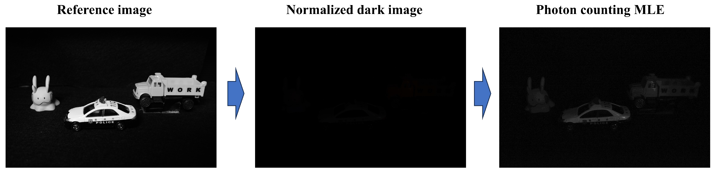
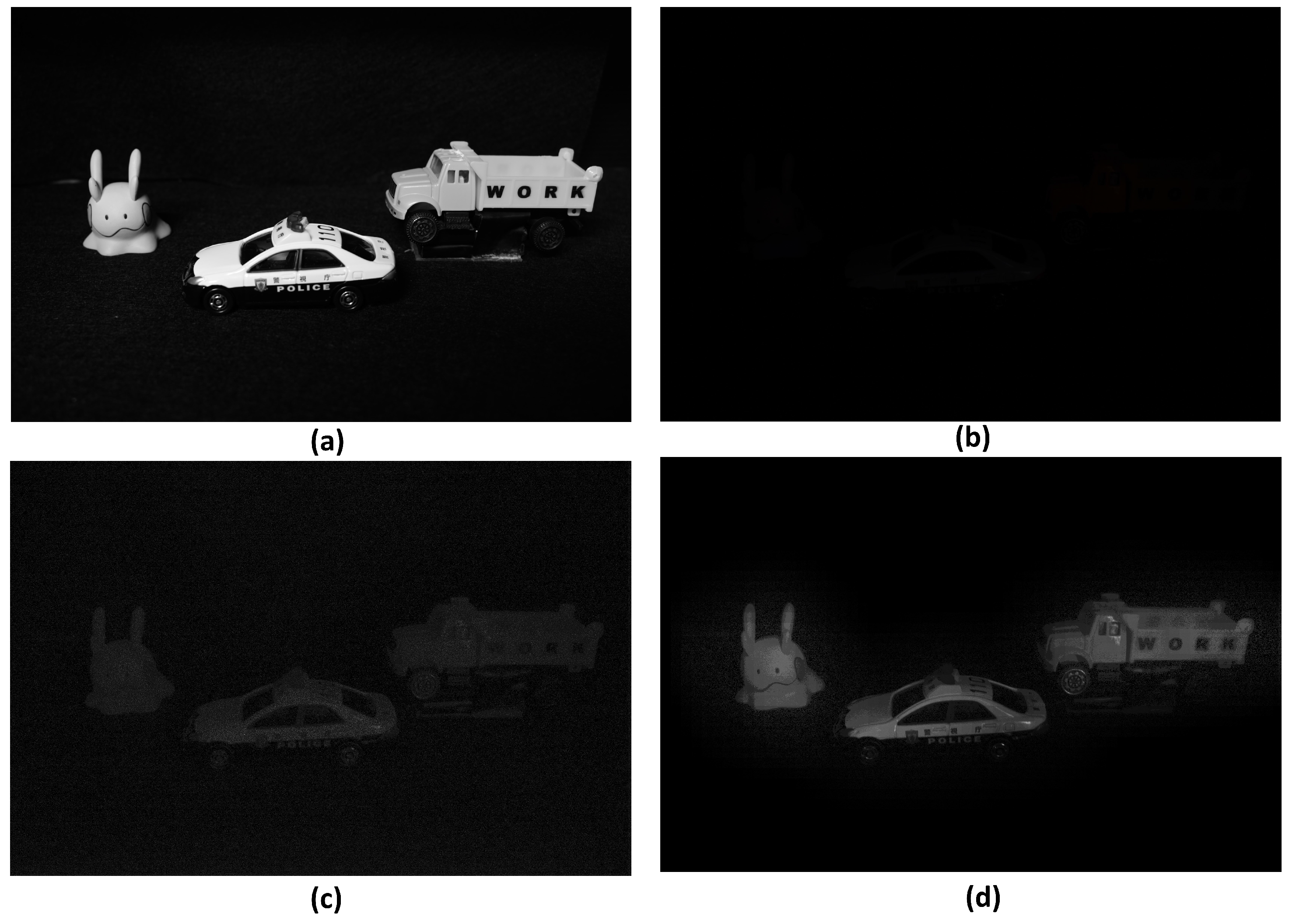
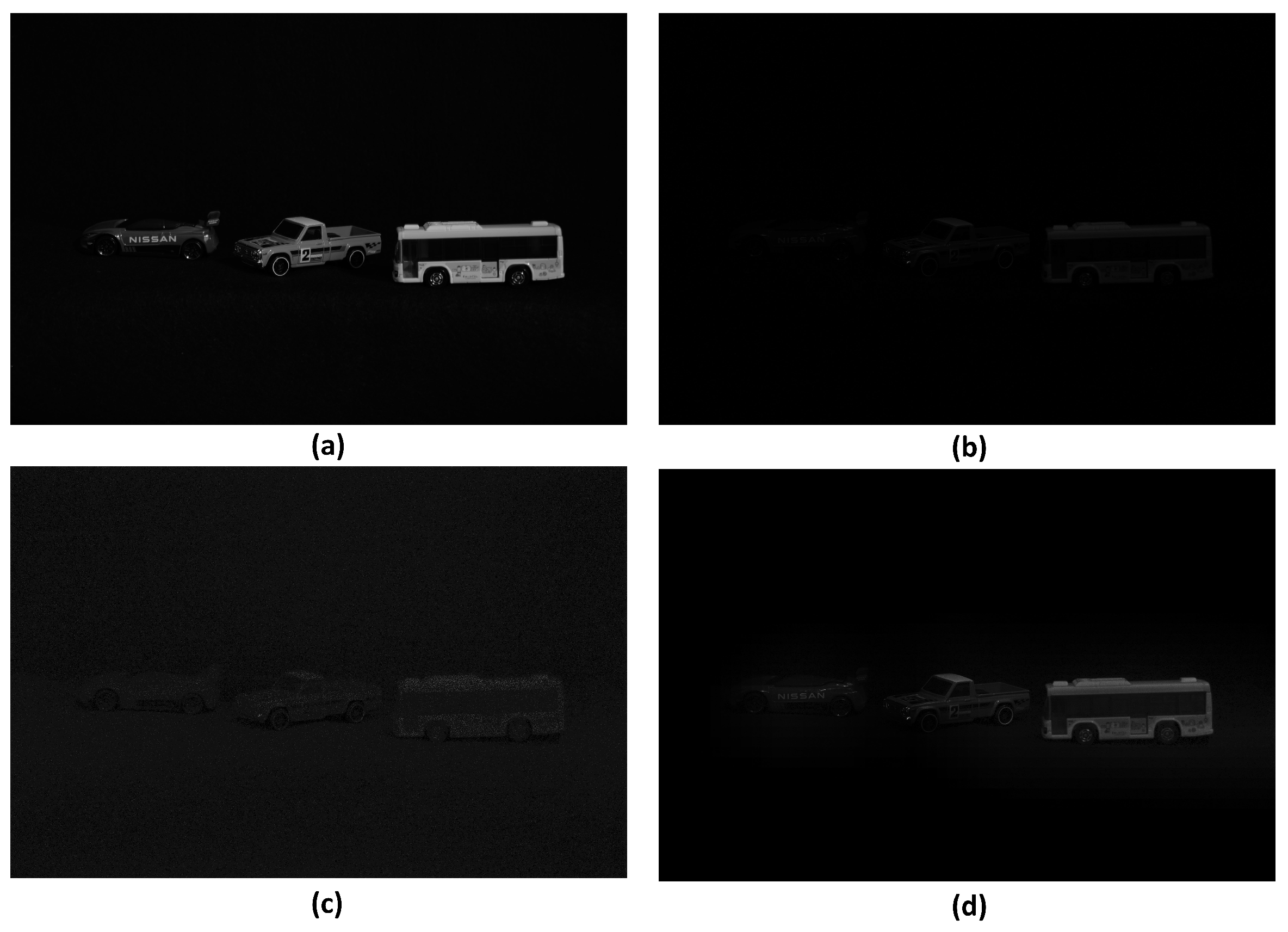
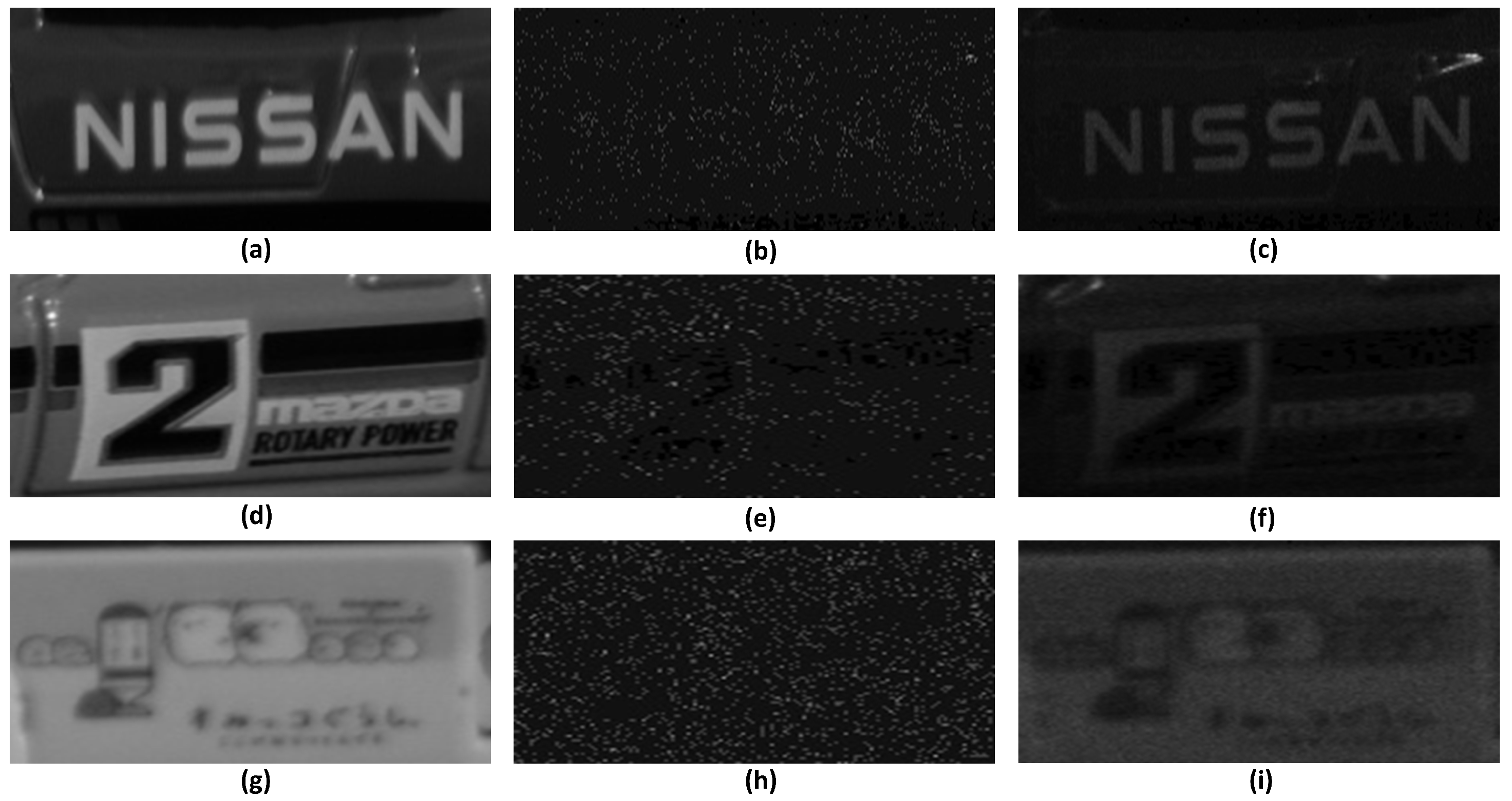
2.2. Proposed Method

To remove background noise from conventional photon-counting imaging techniques, we propose a novel photon-counting method to classify object location and the number of photons by section (COLaNoPS). The proposed method, COLaNoPS, estimates photons in the section where an object is located by calculating the overall intensity of the section rather than applying Poisson random distribution in all areas, and visualizes it by applying a Poisson distribution only where the object is located to prevent generating noise in the background. Furthermore, spatial overlap is used in areas where photons overlap as the section moves, improving the image quality of objects and the recognition rate of objects. The proposed method assumes that the overall intensity value of the section in the presence of the object is higher than in the absence of the object. The method for estimating the location of an object calculates the overall intensity of the section and the overall intensity of the image as a section of a certain size is moved. By comparing the background pixel intensity to the object pixel intensity, we define the threshold for the presence of the object using the median value. The thresholds for determining the presence of an object are as follows.
I i n t e n x , y = k = 0 k 1 l = 0 L 1 I k l a n d K i n t e n x , y = k = 0 k 1 l = 0 L 1 K k l
γ m ( x , y ) = M e d K i n t e n x , y I i n t e n x , y × 100
μ p = { N p , K i n t e n x , y > γ m x , y 0 , K i n t e n x , y γ m x , y ,
where I i n t e n ( x , y ) is the overall pixel intensity of the original image and K i n t e n ( x , y ) is the overall pixel intensity of the section. γ m is the threshold to determine the presence of the object, μ p is the estimated number of photons in the object based on the threshold, and N p is the expected number of photons in each elemental image. The presence of an object is determined based on a defined threshold to estimate photons in the object.
λ ^ k l M A P = C ^ k l + α μ p 1 + β , μ p 0
C ˜ k l μ p λ ^ k l M A P P o i s s o n μ p λ ^ k l M A P .
Using Equations (14) and (15), we can calculate the posterior distribution and estimator of the area in which the object exists. λ ^ k l M A P is the posterior mean of the photons estimated in the object by the Bayesian approach MAP method, and C ˜ k l is the photon estimated from the object of each elemental image. The area in which the object exists is modeled using an estimated posterior mean. As a result, we can define a posterior mean from the MAP method of the photons estimated in the area where the object exists.
R x , y = 1 O s p a t i a l x , y i = 0 N x 1 j = 0 N y 1 λ ^ i j M A P x S i , y S j , N i j > S i j ,
where R is the elemental image reconstructed by the COLaNoPS method; O s p a t i a l is the matrix of spatial overlaps of photons in the object as the section moves; and S i and S j is the section’s x and y-axis shifting pixel, respectively. Finally, the photon-counting imaging technique is applied only to the areas that are estimated to be objects; where photons overlap, the image can be reconstructed by applying the spatial overlapping.
Figure 4 illustrates a flowchart of the COLaNoPS method. We use the median value to define a threshold for the presence of an object, and we calculate the spatial overlap in the space where photons overlap due to section movement. Finally, we visualize the image by estimating the photons for the object under photon-starved conditions.
Figure 5 shows the results of the conventional photon-counting imaging technique and the proposed COLaNoPS method under photon-starved conditions, and shows that the COLaNoPS method improves the image quality of objects more than the conventional photon-counting imaging technique.

3. Experimental Setup and Results

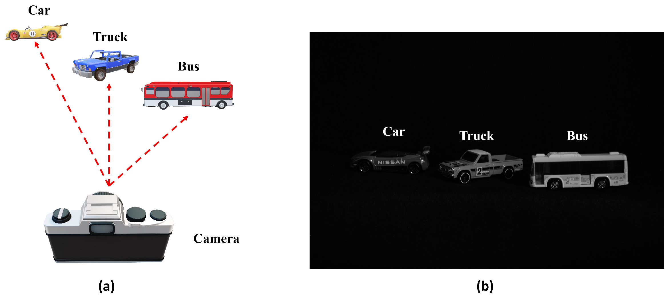
3.1. Experimental Setup
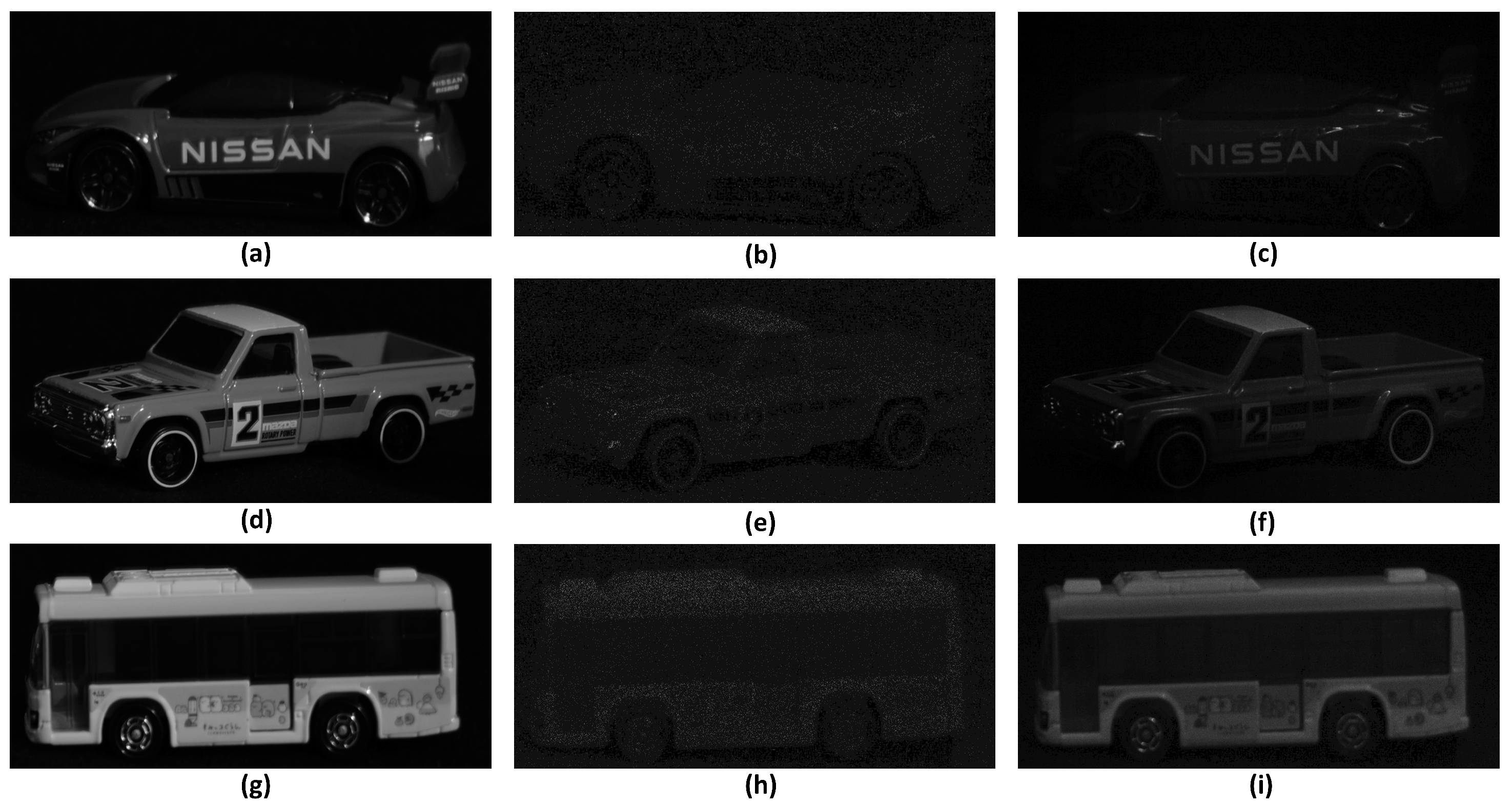
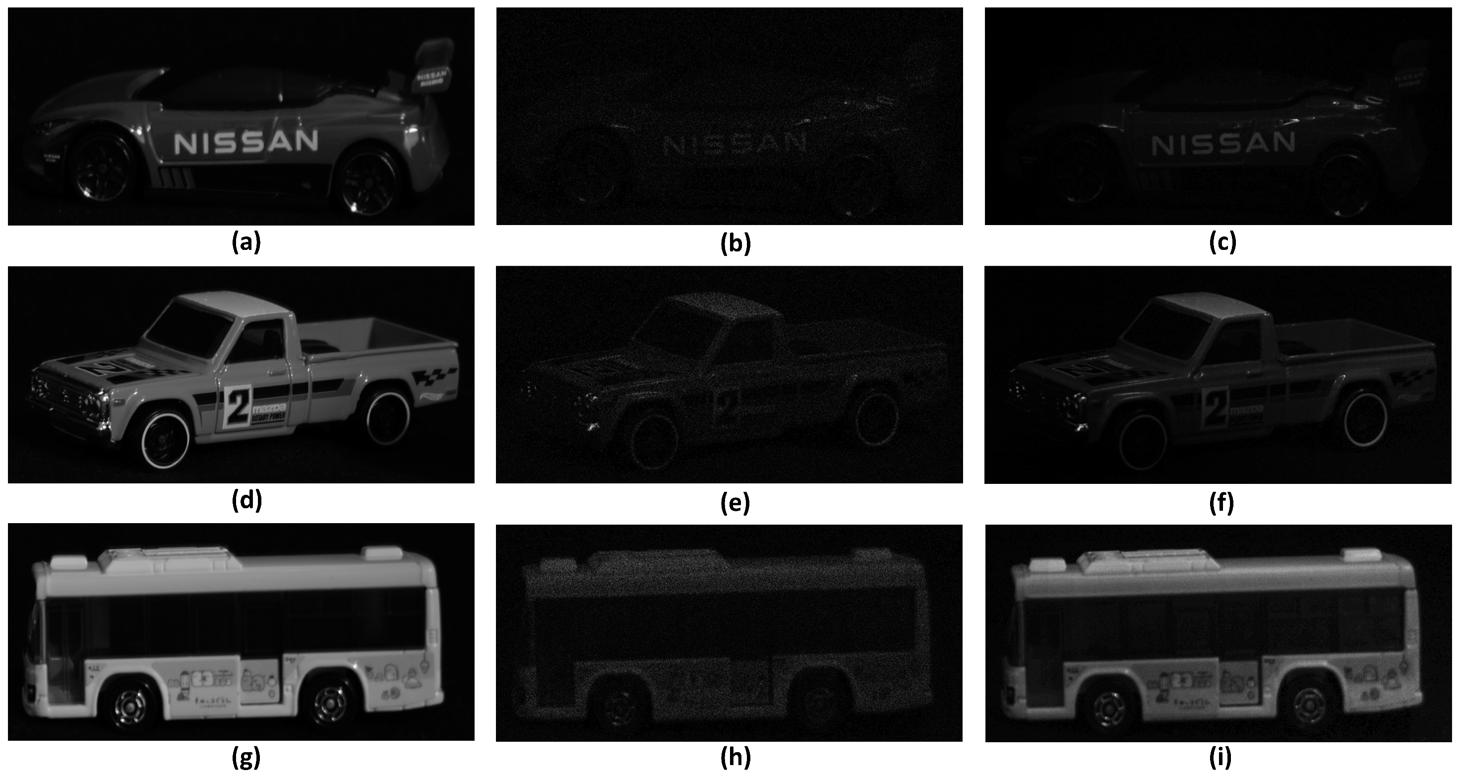
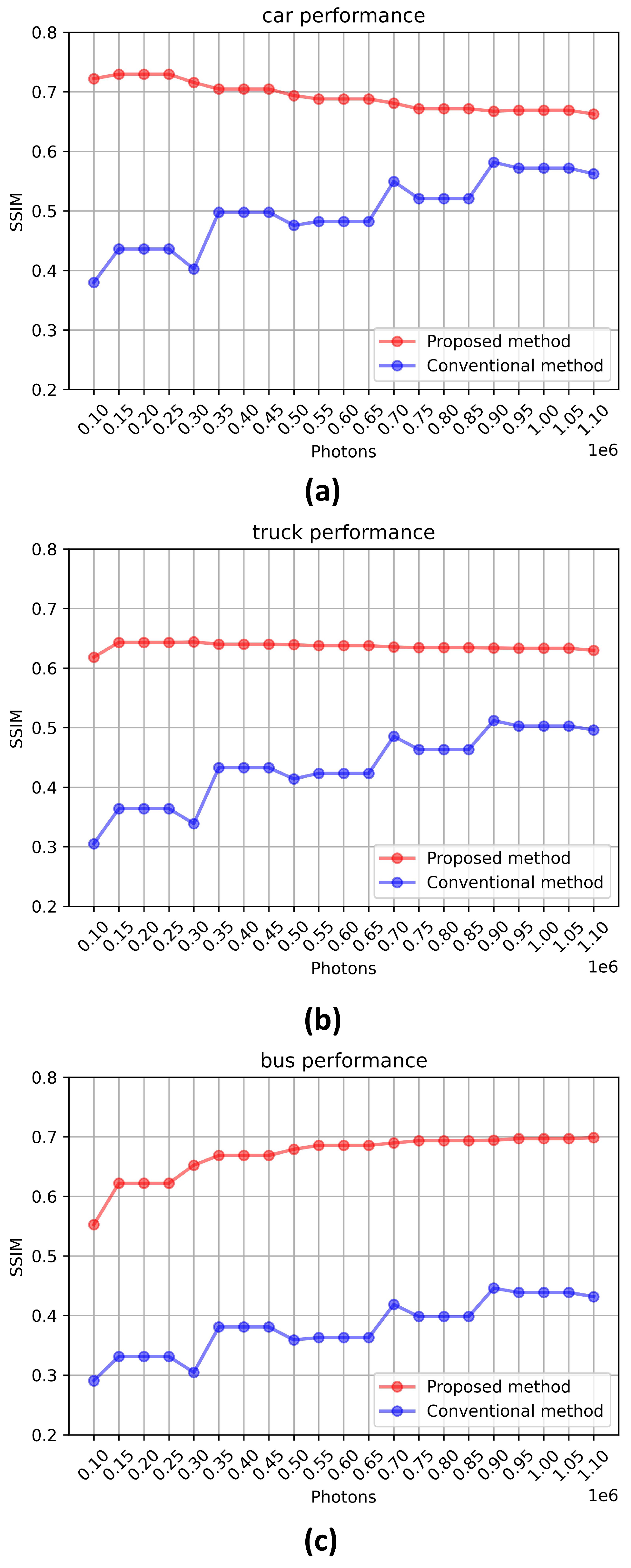
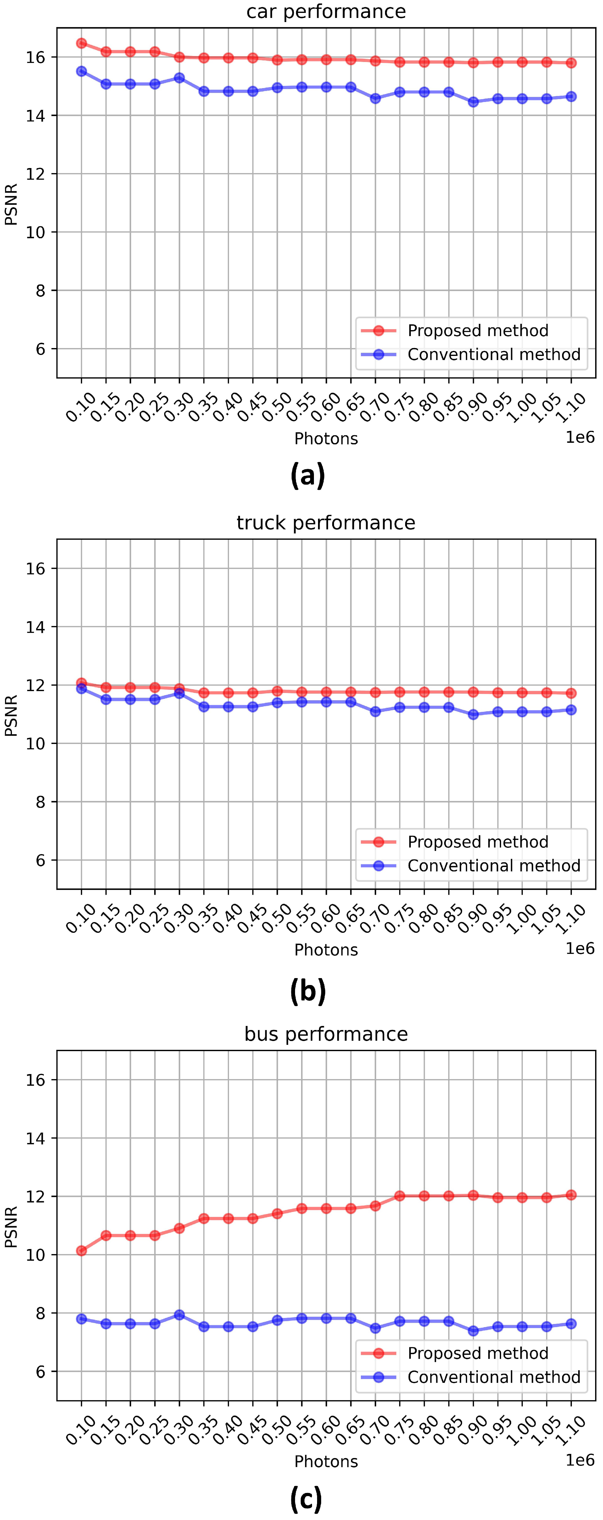
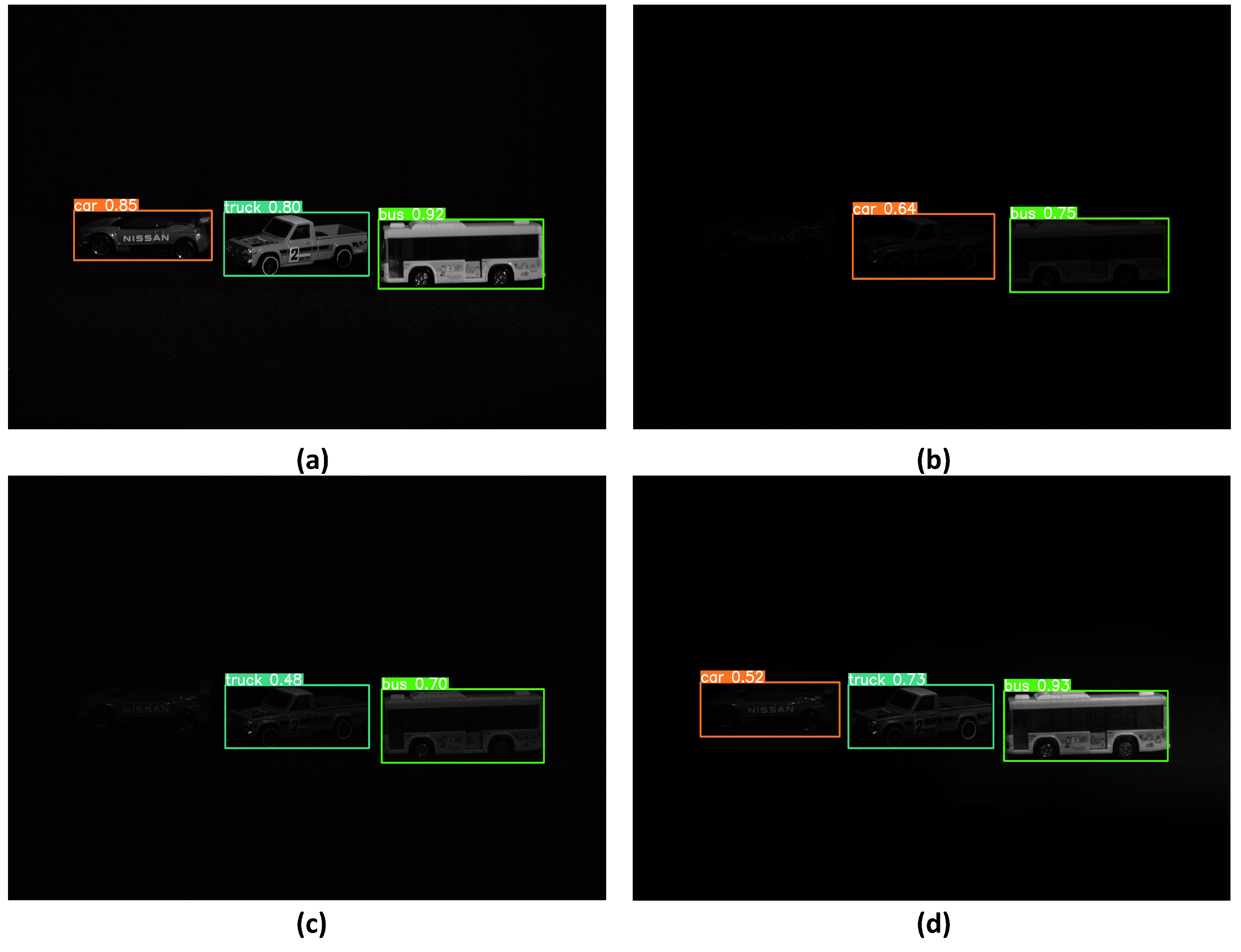
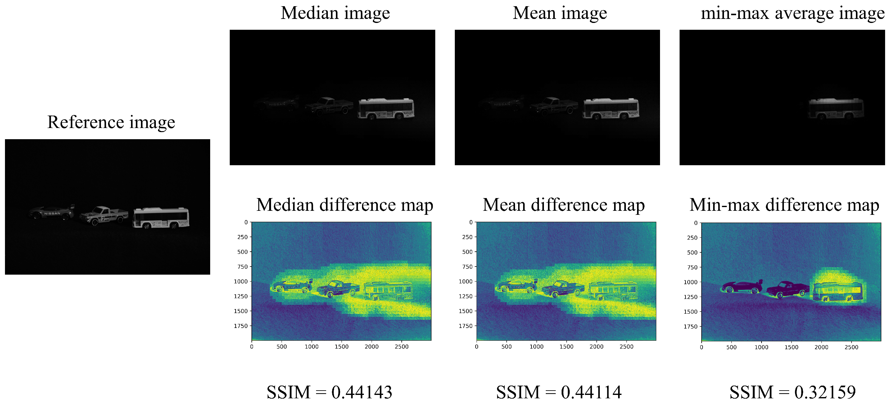
In this subsection, we describe the experimental setup to compare the conventional photon-counting imaging technique with the COLaNoPS method. Figure 6a shows the experimental setup in this paper. Figure 6b is the image obtained by the experimental setup. Photon-starved conditions are set by controlling the amount of light in this experiment. In this experiment, we use a Nikon D5300 to take experimental scenes because our proposed method is the computational algorithm with a general camera to implement photon-counting imaging technique as we mentioned earlier in the first section. All three objects are metal objects, and they are located at different distances from the camera. The distances from the camera to the objects are 400 mm, 430 mm, and 460 mm, with a distance difference of 30 mm for each object.
Table 1 shows the specifications and setup of the camera used in this experiment. The number of photons is gradually increased from 100,000 to 1,100,000 based on images obtained under photon-starved conditions.

3.2. Results

In this subsection, we show the results of the conventional method and the proposed method. Figure 7a is the image obtained under normal light conditions, and Figure 7b is the image obtained under photon-starved conditions. As shown in Figure 7b, the object cannot be visualized because it is too dark. Figure 7c is the reconstruction result by applying conventional photon-counting imaging techniques to the image in Figure 7b, which is not visible to the human eye. Figure 7d shows the reconstruction result by applying the COLaNoPS technique to the image in Figure 7b. For fair comparison, the number of photons applied to the images in Figure 7c and Figure 7d is 100,000. As a result, the reconstructed result by the conventional photon-counting imaging technique as shown in Figure 7c can visualize the object better than the image in Figure 7b, but it cannot accurately recognize the object due to the insufficient number of estimated photons. In contrast, the reconstruction result obtained using the COLaNoPS method as shown in Figure 7d can visualize the object better than the reconstruction result in Figure 7c, and the object can be visualized more clearly than the conventional photon-counting imaging technology when the same number of photons is estimated.
Figure 8 shows the background noise generated by the conventional photon-counting imaging method and the proposed method, and shows the improvement in the quality of the objects. In this experiment, we increase the brightness by 40% and decrease the contrast by 40% to visualize the background noise and object noise. Figure 8a is the result of the conventional photon-counting imaging technique. It shows the random noise in the background as the Poisson distribution is applied in all areas. Furthermore, objects cannot be accurately recognized when the number of estimated photons is insufficient. Figure 8b is the result of the COLaNoPS method. It shows that the background noise is also removed by applying the Poisson distribution only to the area where the object exists. Furthermore, by applying spatial overlap to the areas where photons overlap as the section moves, the object can be visualized more clearly and accurately than the result obtained using the conventional photon-counting imaging technique as shown in Figure 8a.
Figure 9 shows the images reconstructed for each object by the conventional photon-counting imaging technique and the COLaNoPS method, where the number of photons is 100,000. Figure 9a,d,g show reference images obtained under normal light conditions. The objects are listed in the order of car, truck, and bus. All of them are identifiable. Figure 9b,e,h show the results of applying the conventional photon-counting imaging technology. The insufficient photon count estimation makes it difficult to identify the object. Figure 9c,f,i is the result of applying the COLaNoPS method. As shown in Figure 9, in the conventional method, the numbers or letters cannot be recognized accurately due to random noise. On the other hand, we can recognize numbers or letters accurately using the proposed method.
Figure 10 shows the result of increasing the number of photons by 1,100,000. Figure 10a,d,g show the reference image obtained under normal light conditions. The objects are listed in the order of car, truck, and bus, and all of them are identifiable. Figure 10b,e,h show the result of applying the conventional photon-counting imaging technology. The objects are listed in the order of car, truck, and bus, and it is difficult to identify them due to the lack of estimated photons, similar to Figure 9. Figure 10c,f,i show the result of applying the COLaNoPS method. The objects are listed in the same order and the objects can be recognized. As shown in the results of Figure 9 and Figure 10, we can see that, as the number of assumed photons increases, the photons for the object are more accurately estimated. As a result, our proposed method can reduce the background noise and visualize the letters or numbers on the surface of the object more accurately than the conventional photon-counting imaging technique.
Although it is noticed that the proposed method can reconstruct the image under photon-starved conditions more accurately than the conventional method, the numerical comparison analysis may be required to verify our proposed method. In this paper, we use the structural similarity index measure (SSIM) metric for numerical comparison [27]. In SSIM analysis, we measured the change in SSIM as we incremented the photons from 100,000 to 1,100,000. Figure 11 shows the SSIM results for the conventional photon-counting imaging technique and the COLaNoPS method via various numbers of photons. Figure 11a shows the performance metrics of SSIM on car images. The average SSIM of the proposed method is 0.6917, while that of the conventional method is 0.4987, and there is a difference of about 1.387 times. Figure 11b shows the performance metrics of SSIM on truck images, where the average SSIM of the proposed method is 0.6363 and that of the existing method is 0.4336, and a difference of about 1.467 times. Figure 11c shows the performance metrics of SSIM for bus images, and the average SSIM of the proposed method is 0.6697, while that of the existing method is 0.3801, a difference of about 1.761 times. It can be seen that the SSIM value increases with the position of the object, because the closer the object is, the more photons can be estimated, so the image can be reconstructed clearly. However, photon-counting imaging cannot accurately estimate photons for dark objects, and dark objects are subject to frequent random noise. As a result, dark objects such as cars and trucks have a lower SSIM. As shown in Figure 11, the proposed method in this paper shows better SSIM results than the conventional method.
Figure 12 shows the reconstructed images for each object using the conventional photon-counting imaging technique and the COLaNoPS method with 100,000 photons. Figure 12a,d,g show the reference images obtained under normal lighting conditions and show a magnified image of the numbers or letters on objects. Figure 12 b,e,h show the results of applying the conventional photon-counting imaging technique. It is difficult to identify the numbers or letters on objects due to insufficient photons. Figure 12c,f,i present the results of applying the COLaNoPS technique. As shown in Figure 12, the numbers or letters cannot be recognized accurately with the conventional method due to random noise, while they can be recognized accurately with the proposed method.
Figure 13 uses the peak signal-to-noise ratio (PSNR) [28] metric to compare numbers and letters on objects. In the PSNR analysis, we measured the change in PSNR when the number of photons increased from 100,000 to 1,100,000. Figure 13 shows the PSNR results of the conventional photon-counting imaging technique and the COLaNoPS method for different numbers of photons. Figure 13a shows the performance metric of PSNR for the image of letters on the car. The average PSNR of the proposed method is 15.94 and that of the conventional method is 14.85. Their difference is about 1.073 times. Figure 13b shows the performance metrics of PSNR for numbers or letters on the truck, where the average PSNR of the proposed method is 11.78 and that of the conventional method is 11.31. Their difference is about 1.041 times. Figure 13c shows the performance metrics of PSNR for characters on the bus, where the average PSNR of the proposed method is 11.44 and that of the traditional method is 7.647. Their difference is about 1.497 times. As shown in Figure 13, the proposed method in this paper shows better PSNR results than the traditional method.
Figure 14 shows the object recognition rate by applying the YOLOv5 model [29] to the results of the conventional photon-counting imaging technology and the COLaNoPS method. Figure 14a shows the recognition rate of objects for the image obtained under normal light conditions, where all objects are correctly recognized with a high recognition rate. Figure 14b shows the object recognition rates for images obtained under photon-starved conditions. Only the bus object is correctly recognized, and the truck is incorrectly recognized as a car. Figure 14c shows the recognition rate of objects for the reconstructed image using the conventional photon-counting imaging technology. Only the truck and bus objects are recognized, and it shows that the recognition rate of the two objects is low. Figure 14d shows the recognition rate of objects for the image reconstructed using COLaNoPS technology. It can be seen that all objects, such as car, truck, and bus, are recognized more accurately, and the recognition rate is higher than that of the conventional photon-counting imaging technique.
Finally, the proposed method removes background noise by applying a Poisson distribution only to the areas where objects exist under photon-starved conditions, and improves image quality by applying spatial overlap. As a result, the object can be visualized by estimating only the photons for the object, and the recognition rate of the object can be improved.

4. Conclusions

In this paper, we have proposed the COLaNoPS method to remove random noise from the background by estimating only photons for an object under photon-starved conditions. The proposed method has solved the background noise problem by calculating the total intensity of the background and the total intensity of the object as the section moves to estimate where the object exists, and applying spatial overlap to the areas where photons overlap. In addition, to verify the effect of the proposed method, we have compared the numerical analysis of the proposed method using SSIM performance metrics and the YOLOv5 model. As a result, the proposed method has been able to accurately estimate photons only for an object better than the conventional method, and improves the image quality of the object and can improve the object recognition rate of deep learning techniques.
In this experiment, we have applied the median, mean value, and the average of the maximum and minimum values to define the threshold for determining the presence of an object, and found that the median value can accurately classify the object. Figure 15 shows the difference in SSIM among median, mean, and min-max average. The median and mean values can classify the objects correctly, and we can see that the SSIM for the median value is slightly higher than that for the mean value. The min-max average does not classify correctly, so only the bus is visualized. Furthermore, we can see that the min-max average has the lowest SSIM.
The proposed method is expected to contribute to the overall development of technologies utilizing photon energy, including astrophotography, medical imaging, photon encryption, autonomous driving, and AR/VR technologies.
The method proposed in this paper is a technology that visualizes 2D images in a situation where the number of photons is insufficient, but it can be visualized as a 3D image, and it is judged that the distance information of the object and the image quality of the object can be improved when reconstructed as a 3D image [30,31,32].

Author Contributions

Writing—original draft preparation, J.-U.H.; Data curation, H.-W.K.; Conceptualization, J.-U.H. and M.C.; Writing—review and editing, M.C.; Supervision, M.-C.L. All authors have read and agreed to the published version of the manuscript.

Funding

This work was supported under the framework of international cooperation program managed by the National Research Foundation of Korea (NRF-2022K2A9A2A08000152, FY2022) and this work was supported by Kyushu Institute of Technology, On-campus Support Program 2023.

Data Availability Statement

All data underlying the results are available as part of the article and no additional source data are required.

Conflicts of Interest

The authors declare no conflicts of interest.

References

  1. Morton, G. Photon counting. Appl. Opt. 1968, 7, 1–10. [Google Scholar] [CrossRef] [PubMed]
  2. Kröger, H.; Schmidt, G.; Pailer, N. Faint object camera: European contribution to the Hubble Space Telescope. Acta Astronaut. 1992, 26, 827–834. [Google Scholar] [CrossRef]
  3. Brandt, J.; Heap, S.; Beaver, E.; Boggess, A.; Carpenter, K.; Ebbets, D.; Hutchings, J.; Jura, M.; Leckrone, D.; Linsky, J.; et al. The Goddard high resolution spectrograph: Instrument, goals, and science results. Publ. Astron. Soc. Pac. 1994, 106, 890. [Google Scholar] [CrossRef]
  4. Adorf, H.M. Hubble space telescope image restoration in its fourth year. Inverse Probl. 1995, 11, 639. [Google Scholar] [CrossRef]
  5. Sirianni, M.; Jee, M.; Benítez, N.; Blakeslee, J.; Martel, A.; Meurer, G.; Clampin, M.; De Marchi, G.; Ford, H.; Gilliland, R.; et al. The photometric performance and calibration of the Hubble Space Telescope Advanced Camera for Surveys. Publ. Astron. Soc. Pac. 2005, 117, 1049. [Google Scholar] [CrossRef]
  6. Freedman, W.L.; Madore, B.F.; Gibson, B.K.; Ferrarese, L.; Kelson, D.D.; Sakai, S.; Mould, J.R.; Kennicutt, R.C., Jr.; Ford, H.C.; Graham, J.A.; et al. Final results from the Hubble Space Telescope key project to measure the Hubble constant. Astrophys. J. 2001, 553, 47. [Google Scholar] [CrossRef]
  7. Riess, A.G.; Yuan, W.; Macri, L.M.; Scolnic, D.; Brout, D.; Casertano, S.; Jones, D.O.; Murakami, Y.; Anand, G.S.; Breuval, L.; et al. A comprehensive measurement of the local value of the Hubble constant with 1 km s-1 Mpc-1 uncertainty from the Hubble Space Telescope and the SH0ES team. Astrophys. J. Lett. 2022, 934, L7. [Google Scholar] [CrossRef]
  8. Richmond, C. Sir Godfrey Hounsfield. BMJ Brit. Med. J. 2004, 329, 687. [Google Scholar] [CrossRef]
  9. Buzug, T.M. Computed tomography. In Springer Handbook of Medical Technology; Springer: Titisee, Germany, 2011; pp. 311–342. [Google Scholar]
  10. Willemink, M.J.; Persson, M.; Pourmorteza, A.; Pelc, N.J.; Fleischmann, D. Photon-counting CT: Technical principles and clinical prospects. Radiology 2018, 289, 293–312. [Google Scholar] [CrossRef]
  11. Flohr, T.; Petersilka, M.; Henning, A.; Ulzheimer, S.; Ferda, J.; Schmidt, B. Photon-counting CT review. Physica Med. 2020, 79, 126–136. [Google Scholar] [CrossRef]
  12. Tortora, M.; Gemini, L.; D’Iglio, I.; Ugga, L.; Spadarella, G.; Cuocolo, R. Spectral photon-counting computed tomography: A review on technical principles and clinical applications. J. Imaging 2022, 8, 112. [Google Scholar] [CrossRef] [PubMed]
  13. Leng, S.; Bruesewitz, M.; Tao, S.; Rajendran, K.; Halaweish, A.F.; Campeau, N.G.; Fletcher, J.G.; McCollough, C.H. Photon-counting detector CT: System design and clinical applications of an emerging technology. Radiographics 2019, 39, 729–743. [Google Scholar] [CrossRef] [PubMed]
  14. Kreisler, B. Photon counting Detectors: Concept, technical Challenges, and clinical outlook. Eur. J. Radiol. 2022, 149, 110229. [Google Scholar] [CrossRef] [PubMed]
  15. Hsieh, S.S.; Leng, S.; Rajendran, K.; Tao, S.; McCollough, C.H. Photon counting CT: Clinical applications and future developments. IEEE Trans. Radiat. Plasma Med. Sci. 2020, 5, 441–452. [Google Scholar] [CrossRef] [PubMed]
  16. Myung, I.J. Tutorial on maximum likelihood estimation. J. Math. Psychol. 2003, 47, 90–100. [Google Scholar] [CrossRef]
  17. Guillaume, M.; Melon, P.; Réfrégier, P.; Llebaria, A. Maximum-likelihood estimation of an astronomical image from a sequence at low photon levels. J. Opt. Soc. Am. A 1998, 15, 2841–2848. [Google Scholar] [CrossRef]
  18. Aloni, D.; Stern, A.; Javidi, B. Three-dimensional photon counting integral imaging reconstruction using penalized maximum likelihood expectation maximization. Opt. Express 2011, 19, 19681–19687. [Google Scholar] [CrossRef]
  19. Bassett, R.; Deride, J. Maximum a posteriori estimators as a limit of Bayes estimators. Math. Program. 2019, 174, 129–144. [Google Scholar] [CrossRef]
  20. Kuin, N.; Rosen, S. The measurement errors in the Swift-UVOT and XMM-OM. Mon. Not. R. Astron. Soc. 2008, 383, 383–386. [Google Scholar] [CrossRef]
  21. Lee, J.; Kurosaki, M.; Cho, M.; Lee, M.C. Noise Reduction for Photon Counting Imaging Using Discrete Wavelet Transform. J. Inf. Commun. Converg. Eng. 2021, 19, 276–283. [Google Scholar]
  22. Kim, H.W.; Cho, M.; Lee, M.C. Three-Dimensional (3D) Visualization under Extremely Low Light Conditions Using Kalman Filter. Sensors 2023, 23, 7571. [Google Scholar] [CrossRef] [PubMed]
  23. Lee, J.; Cho, M. Enhancement of three-dimensional image visualization under photon-starved conditions. Appl. Opt. 2022, 61, 6374–6382. [Google Scholar] [CrossRef] [PubMed]
  24. Tavakoli, B.; Javidi, B.; Watson, E. Three dimensional visualization by photon counting computational integral imaging. Optics Express 2008, 16, 4426–4436. [Google Scholar] [CrossRef] [PubMed]
  25. Markman, A.; Javidi, B.; Tehranipoor, M. Photon-counting security tagging and verification using optically encoded QR codes. IEEE Photonics J. 2013, 6, 1–9. [Google Scholar] [CrossRef]
  26. Markman, A.; Javidi, B. Full-phase photon-counting double-random-phase encryption. JOSA A 2014, 31, 394–403. [Google Scholar] [CrossRef]
  27. Wang, Z.; Bovik, A.C.; Sheikh, H.R.; Simoncelli, E.P. Image quality assessment: From error visibility to structural similarity. IEEE Trans. Image Process 2004, 13, 600–612. [Google Scholar] [CrossRef]
  28. Gonzalez, R.C.; Woods, R.E. Digital Image Processing, 4th ed.; Pearson: New York, NY, USA, 2018. [Google Scholar]
  29. Jiang, P.; Ergu, D.; Liu, F.; Cai, Y.; Ma, B. A Review of Yolo algorithm developments. Procedia Comput. Sci. 2022, 199, 1066–1073. [Google Scholar] [CrossRef]
  30. Lee, J.; Cho, M.; Lee, M.C. 3D Visualization of Objects in Heavy Scattering Media by Using Wavelet Peplography. IEEE Access 2022, 10, 134052–134060. [Google Scholar] [CrossRef]
  31. Hong, S.H.; Jang, J.S.; Javidi, B. Three-dimensional volumetric object reconstruction using computational integral imaging. Opt. Express 2004, 12, 483–491. [Google Scholar] [CrossRef]
  32. Schulein, R.; DaneshPanah, M.; Javidi, B. 3D imaging with axially distributed sensing. Opt. Lett. 2009, 34, 2012–2014. [Google Scholar] [CrossRef]
Figure 1. Computational photon-counting imaging by MLE.
Electronics 13 00038 g001
Figure 2. Reconstructed images by photon-counting imaging system under photon-starved conditions. (a) Reference image, (b) image obtained under photon-starved conditions, (c) image reconstructed by MLE, and (d) image reconstructed by MAP, where N p is 400,000.
Electronics 13 00038 g002
Figure 3. Problem with the background noise of photon-counting imaging.
Electronics 13 00038 g003
Figure 4. Flow chart of COLaNoPS.
Electronics 13 00038 g004
Figure 5. COLaNoPS method results. (a) Reference image, (b) image obtained under photon-starved conditions, (c) conventional photon-counting image with Bayesian approach, and (d) reconstructed image by COLaNoPS, where N p is 400,000.
Electronics 13 00038 g005
Figure 6. (a) Experimental setup and (b) the image obtained by the experimental setup.
Electronics 13 00038 g006
Figure 7. Reconstruction results. (a) Reference image, (b) image obtained under photon-starved conditions, (c) image reconstructed by the conventional photon-counting imaging with Bayesian, and (d) image reconstructed by COLaNoPS method, where N p is 100,000.
Electronics 13 00038 g007
Figure 8. Comparison of the noise of the background and the object. (a) Conventional photon-counting image and (b) COLaNoPS method image, where N p is 100,000.
Electronics 13 00038 g008
Figure 9. Cropped object images, where objects are car, truck, and bus. (a,d,g) are the reference images obtained under normal light conditions; (b,e,h) are images obtained using the conventional photon-counting imaging technique; and (c,f,i) are images obtained using our proposed method, where N p is 100,000.
Electronics 13 00038 g009
Figure 10. Cropped object images, where objects are car, truck, and bus.(a,d,g) are reference images obtained under normal light conditions; (b,e,h) are images obtained using the conventional photon-counting imaging technique; and (c,f,i) are images obtained using our proposed method, N p is 1,100,000.
Electronics 13 00038 g010
Figure 11. SSIM comparison for (a) car, (b) truck, and (c) bus images.
Electronics 13 00038 g011
Figure 12. Magnified image of the number or character on the object. (a,d,g) are reference images obtained under normal light conditions; (b,e,h) are images obtained using the conventional photon-counting imaging technique; and (c,f,i) are images obtained using our proposed method, where N p is 100,000.
Electronics 13 00038 g012
Figure 13. PSNR comparison for (a) car, (b) truck, and (c) bus images.
Electronics 13 00038 g013
Figure 14. Object recognition result by YOLOv5. (a) Reference image, (b) image obtained under photon-starved conditions, (c) image reconstructed using conventional photon-counting imaging, and (d) image reconstructed using the COLaNoPS method, where N p is 5,984,000.
Electronics 13 00038 g014
Figure 15. Result of the SSIM for the median, mean, and min-max average.
Electronics 13 00038 g015
Table 1. Camera specifications and setup.
SetupNikon D5300
Resolution2992 × 2000
Sensor size23.5 mm × 15.7 mm
Section size400 × 400
Section shifting pixel50
Focal length5 mm
ISO160
Shutter speedNormal5 s
Extremely low-light180 s
Disclaimer/Publisher’s Note: The statements, opinions and data contained in all publications are solely those of the individual author(s) and contributor(s) and not of MDPI and/or the editor(s). MDPI and/or the editor(s) disclaim responsibility for any injury to people or property resulting from any ideas, methods, instructions or products referred to in the content.

