Application of an Output Filtering Method for an Unstable Wheel-Driven Pendulum System Parameter Identification

Abstract

This research aims to apply an output filtering method to conduct the system parameter identification of an unstable wheel-driven pendulum system. First, the nonlinear dynamic model of the system is established by utilizing the Lagrangian dynamic theorem. Next, the Least-Square (LS) is introduced for system parameter identification formulation. Nevertheless, considering the real scenario, the wheel displacement is acquired from encoders subject to quantization errors. The pitch angle of the pendulum cart is also accompanied by Gaussian noise. Therefore, using numerical differentiation for angular acceleration in the LS estimations directly would induce incorrect state information seriously. To address this practical issue, an output filtering method is considered. The developed parameter identification algorithm could attenuate the influence of the quantization effect as well as noisy data and thus obtain much more accurate parameter identification results. Comparative simulation reveals that the output filtering method has a superior parameter estimation performance than the direct numerical difference method.

1. Introduction

System parameter identification (SPI) uses the input and output histories to establish to describe its dynamic behavior [1,2,3,4]. Several data-driven identification methods for a nonlinear mechanical system can be found in [5,6]. The reason why SPI is important is that system parameters coupling with states would have a great effect on the system’s dynamic response. Namely, those parameters represent the system’s features. If those parameters can be identified accurately, it is without a doubt that the procedure of designing a control law will become more time-saving, efficient, and robust.

Nevertheless, without an accurate dynamic model, all attempts at parameter identification and rule-based controller designs are inefficient or even futile. Thus, establishing an accurate system model becomes the primary step. In the past decade, significant progress has been made in the research on self-stabilizing two-wheeled robots. Various models and controllers have been employed to interpret and control the dynamics of two-wheeled robots. Further research on the dynamic modeling of two-wheeled robots is also reviewed in [7]. There are several ways to derive the wheel-driven pendulum’s dynamics equation, such as the Newton methods [8] and the Lagrangian dynamic theorem [9]. Among different approaches, this paper adopts the Lagrangian dynamic theorem owing to its systematic formulation procedures. Moreover, due to the unstable nature of an inverted pendulum, a simple PID controller must be applied firstly to stabilize the system’s attitude when conducting the SPI processes.

Secondly, based on the derived model, it can be found that the SPI can be formulated as a standard LS solution. The LS method is widely applied in parameter identifications [10,11]. According to the LS, an over-determined normal equation $\mathbf{Y}\left(t\right)=\Phi \left(t\right)X$ is formulated, where the output vector $\mathbf{Y}\left(t\right)$ and the observation matrix $\mathbf{\Phi }\left(t\right)$ are the key measurements to determine the parameter vector $X$ accurately. To fulfill the observation matrix $\Phi \left(t\right)$, some states need to be estimated through numerical differentiation [12,13]. Nonetheless, from the practical realization point of view, the wheel angle data measured from encoders are subjected to quantization effect. Meanwhile, the measured pitch angle and angular velocity from an orientation sensor, such as the inertial measurement unit (IMU), would accompanied by inevitable Gaussian noise. As pointed out in [14], the measurement noise will be amplified if $Y\left(t\right)$ and $\Phi \left(t\right)$ contain serious noise, which further gives rise to a negative influence on parameter identification.

To address the potential issue discussed above, the filter regression model is applied to the identification methodology for robot manipulators and industrial robots, eliminating the need for either the measurement or off-line calculation of the linear and angular accelerations [15,16,17,18,19]. Inspired by the works [20,21], an output filtering method is considered to tackle this problem and is applied to the unstable wheel-driven pendulum system. The advantage of the presented method is that the observation matrix of the filtering method does not contain the raw noise corrupted measurements, the filtered ones are adopted instead. Moreover, there is no need to involve the acceleration information, which is not directly available from sensors. Refer to the associated studies [22,23]; they present an energy-based regression model that only involves position and velocity. This approach avoids using numerical differentiation for acceleration estimations and applies integration on the joint/motor velocities. However, there is no extra degree of freedom to adjust the pure integration, which can be taken as a special case of a low-pass filter. Therefore, the command trajectories should be properly designed. Recent research [24] has emphasized the significance of coarse encoder quantization errors in angular measurements, which introduce noise affecting the estimation of velocity and acceleration. Consequently, the article addresses this issue by applying the filter-based method. Notably, in comparison to the differentiation-based method found in the existing literature, the filter-based primary feature is its avoidance of direct differentiation for velocity information acquisition. Moreover, the filter-based approach offers a more efficient approach to mitigate the influence of quantization noise. Experimental results presented in [24] affirm that filter-based SPI surpasses differentiation-based SPI in terms of parameter estimation accuracy. However, a simple stable motor system was presented [24]. To exploration the potential capability of the filter-based method, this work applied it to highly nonlinear unstable wheel-driven pendulum system.

Note that the selection of a filtering operator is highly important. A great integral operator should preserve the system’s dominant frequencies and filter out the unwanted noises. Otherwise, the integral operator might distort the dominant frequencies or could not remove the redundant noises. In summary, the importance of SPI mainly includes two parts: first, SPI allows control engineers to develop a robust control law more easily; second, dynamics modeling together with SPI can be used as a digital twin to monitor the system behavior online [25].

The main contributions of the paper are summarized as follows: (1) extending the filter-based SPI to a nonlinear unstable wheel-driven pendulum system; (2) presenting an output filtering method which can suppress the Gaussian noise and quantization noise effects; (3) conducting a performance comparison study between the proposed output filtering method and the direct numerical differentiation method; and (4) demonstrating the use of aggressive command input citation can enhance the precision of the parameter estimations.

2. System Description

The description of the wheel-driven pendulum dynamics model can be found in [26]. Figure 1 shows the position of the system, where ${\theta }_w$ and ${\theta }_p$ are the wheel’s rotational angle, and the inclined angle of the body, respectively. $M$ represents the mass of the body and $m$ denotes the mass of the wheels. $J_w$ and $J_p$ are the moment of inertia with respect to the wheel’s axles of the wheel and the body, respectively. $R$ is the wheel radius. $W$ and $L$ are the distance between two wheels and the distance between the wheel and the center of mass, respectively. The positions of the left and right wheels, and the center of mass are represented by the coordinates $\left(x_i,y_i,z_i\right)$, where $i$ corresponds to $l, r,$ or $b$.

2.1. Modeling of a Wheel-Driven Pendulum Cart

According to the Lagrangian dynamics, it is composed of the kinetic energy $T$ and the potential energy $U$, which can be described as $L=T-U$, in which

$$\begin{array}{c}L=m{R}^2{\dot{\theta }}_w{}^2+\frac{1}{2}M{R}^2{\dot{\theta }}_w{}^2+MR{\dot{\theta }}_w{\dot{\theta }}_{p}L\cos \left({\theta }_p\right)+\frac{1}{2}M{\dot{\theta }}_p{}^2{L}^2+J_w{\dot{\theta }}_w{}^2+\frac{1}{2}{J}_b{\dot{\theta }}_p{}^2+{\epsilon }^2{J}_m{\dot{\theta }}_w{}^2\hfill \\ \hspace{1em}-2{\epsilon }^2{J}_m{\dot{\theta }}_w{\dot{\theta }}_p+{\epsilon }^2{J}_m{\dot{\theta }}_p{}^2-MgR-MgL\cos {\theta }_p\hfill \end{array}$$

(1)

Based on the definition of the Lagrangian dynamics, one has

$$\frac{d}{dt}\left(\frac{\partial L}{\partial {\dot{\theta }}_q}\right)-\frac{\partial L}{\partial {\theta }_q}=F_q$$

(2)

where $q$ denotes the general coordinate, and $F_q$ represents the general force with respect to the general coordinate. Hence, the dynamics equation of a wheel-driven pendulum cart can be written as

$$F_{{\theta }_w}=\left(\left(2m+M\right)R^2+2J_W+2{\epsilon }^2{J}_m\right){\ddot{\theta }}_w+\left(MLR\cos \left({\theta }_p\right)-2{\epsilon }^2{J}_m\right){\ddot{\theta }}_p-MLR{\dot{\theta }}_p{}^2\sin \left({\theta }_p\right)$$

(3)

and

$$F_{{\theta }_p}=\left(MLR\cos \left({\theta }_p\right)-2{\epsilon }^2{J}_m\right){\ddot{\theta }}_w+\left(M{L}^2+J_b+2{\epsilon }^2{J}_m\right){\ddot{\theta }}_p-MgL\sin \left({\theta }_p\right)$$

(4)

where $F_{{\theta }_w}$, $F_{{\theta }_p}$ denotes the generalized force with respect to the general coordinate $\left[\begin{array}{cc}{\theta }_w& {\theta }_p\end{array}\right]$, respectively.

2.2. Model Description of a Motor

The governing equations of the electrical driving circuit and the motor mechanism can be expressed by

$$L\frac{di}{dt}+i{R}_m+K_{e}w=V_{in}$$

(5)

and

$$J_m\frac{dw}{dt}=K_{t}i-B_{m}w-T_L$$

(6)

respectively, in Equation (5), $L$ is the inductance, $R_m$ is the resistance, $K_e$ is the back emf constant, $V_{in}$ is the applied voltage, $i$ is the armature current, and $w$ is the motor’s angular velocity which is equivalent to the wheel’s angular velocity ${\dot{\theta }}_w$. Moreover, in (6), $J_m$ is the motor’s moment of inertia, $K_t$ is the torque constant, $B_m$ is the viscous coefficient, and $T_L$ represents the external load.

According to the property that electric power is equivalent to mechanical power, it follows that $\left(K_{e}w\right)i=\left(K_{t}i\right)w$. Therefore, one has $K_e=K_t:=K$. Since the mechanical dynamics of a wheel-driven pendulum cart are much slower than electrical dynamics, (5) reduces to

$$V_{in}\approx i{R}_m+Kw$$

(7)

Based on (4)–(7), the actuator dynamics can be simplified by

$$J_m\frac{dw}{dt}=\frac{K}{R_m}{V}_{in}-\left(\frac{K^2}{R_m}+B_m\right)w-T_L$$

(8)

The external loads are mainly caused by the friction between the cart’s body and wheels, and also between the wheels and the ground. Moreover, the influence of the motor’s viscosity can be neglected. Thus, $T_L$ can be modeled by

$$T_L=f_m\left({\dot{\theta }}_p-{\dot{\theta }}_w\right)$$

(9)

Substituting (9) into (8) yields

$$J_m\frac{dw}{dt}=F_{{\theta }_w}$$

(10)

in which

$$F_{{\theta }_w}=\alpha V_{in}-2\left(\beta +f_w\right){\dot{\theta }}_w+2\beta {\dot{\theta }}_p$$

(11)

and the equivalent coefficients $\alpha$ and $\beta$ are

$$\begin{array}{l}\alpha =\frac{2\epsilon K_t}{R_m},\\ \beta =\frac{\epsilon K_t{K}_b}{R_m}+f_m\end{array}$$

(12)

Furthermore, because of the inverted pendulum’s physical behavior, it is obvious that $F_{{\theta }_w}=-F_{{\theta }_p}$. Therefore, one has

$$F_{{\theta }_p}=-\alpha V_{in}+2\left(\beta +f_w\right){\dot{\theta }}_w-2\beta {\dot{\theta }}_p$$

(13)

2.3. Integrate the Model of a Pendulum Cart and Motors

Based on (4), (11) and (13), the complete dynamics equations of the wheel-driven pendulum cart can be represented by

$$\begin{array}{c}\alpha V_{in}=2\left(\beta +f_w\right){\dot{\theta }}_w-2\beta {\dot{\theta }}_p-MLR{\dot{\theta }}_p{}^2\sin \left({\theta }_p\right)+\left(\left(2m+M\right)R^2+2J_W+2{\epsilon }^2{J}_m\right){\ddot{\theta }}_w\hfill \\ \hspace{1em}\hspace{1em} +\left(MLR\cos \left({\theta }_p\right)-2{\epsilon }^2{J}_m\right){\ddot{\theta }}_p\hfill \end{array}$$

(14)

and

$$\begin{array}{c}\alpha V_{in}=2\left(\beta +f_w\right){\dot{\theta }}_w-2\beta {\dot{\theta }}_p-\left(M{L}^2+J_b+2{\epsilon }^2{J}_m\right){\ddot{\theta }}_p+MgL\sin \left({\theta }_p\right)\hfill \\ \hspace{1em}\hspace{1em} -\left(MLR\cos \left({\theta }_p\right)-2{\epsilon }^2{J}_m\right){\ddot{\theta }}_w\hfill \end{array}$$

(15)

Apparently, the dynamics of the wheel-driven pendulum are highly nonlinear and unstable. In order to estimate the parameters, the equivalent parameter representation should be further considered. Moreover, since the system is unstable, a stabilizing control law must be applied for the collection of input/output excitation signals.

3. System Parameter Identification

3.1. Least-Square Algorithm

The LS algorithm has been widely used to identify a system’s parameters since this approach enables the provision of a globally optimal solution to minimize the residual error. As a result, the LS algorithm plays an important role in this paper to perform the system parameter identification.

Consider the regression model as $y\left(t\right)=\mathsf{\phi }\left(t\right)X$, in which $y\left(t\right)\in {ℝ}^p$ is the output of the regression model, $\mathsf{\phi }\left(t\right)\in {ℝ}^{p\times n}$ is the regressor, and $X={\left[\begin{array}{ccc}{X}_1& \dots & X_n\end{array}\right]}^T\in {ℝ}^n$ is the unknown parameter vector to be identified.

Based on a sufficiently long period of observation for $t=T, 2T, \cdots , NT$, where $T$ is the sampling interval, it gives the following over-determined equation $Y=\Phi X$, where

$$Y={\left[\begin{array}{c}y\left(T\right)\\ y\left(2T\right)\\ ⋮\\ y\left(NT\right)\end{array}\right]}_{m\times 1}, \Phi ={\left[\begin{array}{c}\mathsf{\phi }\left(T\right)\\ \mathsf{\phi }\left(2T\right)\\ ⋮\\ \mathsf{\phi }\left(NT\right)\end{array}\right]}_{m\times n}$$

(16)

and $m=pN>n$. The LS algorithm aims to determine the estimated parameter $\widehat{X}={\left[\begin{array}{ccc}{\widehat{X}}_1& \dots & {\widehat{X}}_n\end{array}\right]}^T\in {ℝ}^n$ to minimize the residual error $E$, which equals to $\underset{\widehat{X}}{\min }{\Vert E\Vert }^2\triangleq {\Vert Y-\Phi X\Vert }^2$. For the residual error $E$, the optimal solution is

$$\widehat{X}={\left({\Phi }^T\Phi \right)}^{-1}{\Phi }^{T}Y\triangleq {\Phi }^{†}Y$$

(17)

in which ${\Phi }^{†}={\left({\Phi }^T\Phi \right)}^{-1}{\Phi }^T$ is the pseudo-inverse of the observation matrix $\Phi$, and the matrix ${\Phi }^T\Phi$ must be invertible. Moreover, it is worth to note that the identified parameters $\widehat{X}$ will deviate from their references significantly if obvious noise appears in (16).

3.2. Regression Model of a Wheel-Driven Pendulum System

To facilitate the system identification, according to (14) and (15), define $X={\left[X_1,X_2,X_3,X_4,X_5,X_6,X_7\right]}^T$ as follows,

$$\begin{array}{l}{X}_1=\frac{\left(2m+M\right)R^2+2J_w}{\alpha }, X_2=\frac{2\epsilon J_m}{\alpha }, X_3=\frac{MLR}{\alpha },\\ X_4=\frac{M{L}^2+J_b}{\alpha }, X_5=\frac{MgL}{\alpha }, X_6=\frac{2\left(\beta +f_w\right)}{\alpha }, X_7=\frac{2\beta }{\alpha }\end{array}$$

(18)

Based on the equivalent parameter representation (18), Equations (14) and (15) become

$$V_{in}=\left(X_1+X_2\right){\ddot{\theta }}_w+\left(X_3\cos \left({\theta }_p\right)-X_2\right){\ddot{\theta }}_p-X_3{\dot{\theta }}_p{}^2\sin \left({\theta }_p\right)+X_6{\dot{\theta }}_w-X_7{\dot{\theta }}_p$$

(19)

and

$$V_{in}=-\left(X_3\cos \left({\theta }_p\right)-X_2\right){\ddot{\theta }}_w-\left(X_4+X_2\right){\ddot{\theta }}_p-X_5\sin \left({\theta }_p\right)+X_6{\dot{\theta }}_w-X_7{\dot{\theta }}_p$$

(20)

respectively. Next, to apply the LS algorithm, it is necessary to express the unknown system parameters in terms of a linear regression form

$$\mathsf{\tau }\left(t\right)=\mathsf{\phi }\left(t\right)X$$

(21)

in which $\mathsf{\tau }\left(t\right)={\left[V_{in}\left(t\right),V_{in}\left(t\right)\right]}^T$ and

$$\mathsf{\phi }\left(t\right)=\left[\begin{array}{ccccccc}{\ddot{\theta }}_w& {\ddot{\theta }}_w-{\ddot{\theta }}_p& {\phi }_{13}& 0& 0& {\dot{\theta }}_w& -{\dot{\theta }}_p\\ 0& {\ddot{\theta }}_w-{\ddot{\theta }}_p& {\phi }_{23}& -{\ddot{\theta }}_p& {\phi }_{25}& {\dot{\theta }}_w& -{\dot{\theta }}_p\end{array}\right]$$

(22)

where

$$\begin{array}{l}{\phi }_{13}=\cos \left({\theta }_p\right){\ddot{\theta }}_p-\sin \left({\theta }_p\right){\dot{\theta }}_p^2,\\ {\phi }_{23}=-\cos \left({\theta }_p\right){\ddot{\theta }}_w,\\ {\phi }_{25}=\sin \left({\theta }_p\right)\end{array}$$

(23)

Given the sampled data for $t=T, 2T, \cdots , NT$, the LS equation can be constructed by $Y=\Phi X$, where

$$Y={\left[\begin{array}{c}\mathsf{\tau }\left(T\right)\\ \mathsf{\tau }\left(2T\right)\\ ⋮\\ \mathsf{\tau }\left(NT\right)\end{array}\right]}_{2N\times 1}, \Phi ={\left[\begin{array}{c}\mathsf{\phi }\left(T\right)\\ \mathsf{\phi }\left(2T\right)\\ ⋮\\ \mathsf{\phi }\left(NT\right)\end{array}\right]}_{2N\times 7}$$

(24)

Theoretically, the optimal parameters can be obtained by applying the LS solution $\widehat{X}={\Phi }^{†}Y$ to minimize the residual error.

However, an examination of the observation matrix $\mathbf{\Phi }$ reveals that it involves not only the wheel rotation angle and the cart’s pitch angle and angular velocity but also the wheel’s angular velocity, acceleration, and the cart’s pitch angular acceleration. From a practical realization scenario, the wheel rotation angle can be directly measured through an encoder. Nevertheless, the angle measurement is subject to the quantization effect. Simultaneously, the pitch angle and the pitch angular velocity are also measurable by an IMU but are prone to measurement noise. Additionally, the regression matrix (22) includes unmeasurable variables such as the cart’s pitch angular acceleration, wheel angular velocity, and wheel angular acceleration, which must be obtained through numerical differencing. It is well known that the numerical differencing method can significantly amplify the noise. This amplification of measurement noise leads to the problem formulation of the ideal LS from $Y=\Phi X$ to $Y+\Delta Y=\left(\Phi +\Delta \Phi \right)X$, which causes parameter identification bias even using the optimal solution $\widehat{X}={\Phi }^{†}Y$. In other words, the reduction in $\Delta Y$ and $\Delta \Phi$ would effectively contribute to the improvement of parameter identification accuracy. This issue is going to be addressed by applying a filtering based regression model, introduced in the following section.

3.3. Filtering-Based Regression Model

It is well known that the measurement encoder quantization effect as well as the Gaussian noise may be amplified by taking the numerical differentiation. To avoid this potential weakness, the filtering-based regression model is considered. In other words, (21) should be rewritten as

$$\mathsf{\tau }\left(t\right)=\left[\frac{d^2}{d{t}^2}{\mathsf{\phi }}_2\left(t\right)+\frac{d}{dt}{\mathsf{\phi }}_1\left(t\right)+{\mathsf{\phi }}_0\left(t\right)\right]X$$

(25)

in which

$$\begin{array}{l}{\mathsf{\phi }}_2\left(t\right)=\left[\begin{array}{ccccccc}{\theta }_w& {\theta }_w-{\theta }_p& 0& 0& 0& 0& 0\\ 0& {\theta }_w-{\theta }_p& 0& -{\theta }_p& 0& 0& 0\end{array}\right],\\ {\mathsf{\phi }}_1\left(t\right)=\left[\begin{array}{ccccccc}0& 0& \cos \left({\theta }_p\right){\dot{\theta }}_p& 0& 0& {\theta }_w& -{\theta }_p\\ 0& 0& -\cos \left({\theta }_p\right){\dot{\theta }}_w& 0& 0& {\theta }_w& -{\theta }_p\end{array}\right],\\ {\mathsf{\phi }}_0\left(t\right)=\left[\begin{array}{ccccccc}0& 0& 0& 0& 0& 0& 0\\ 0& 0& -\sin \left({\theta }_p\right){\dot{\theta }}_p{\dot{\theta }}_w& 0& \sin \left({\theta }_p\right)& 0& 0\end{array}\right]\end{array}$$

(26)

Taking the Laplace transform of (25) yields

$$\mathsf{\tau }\left(s\right)=\mathsf{\phi }\left(s\right)X$$

(27)

in which $s$ represents the Laplace operator; $\mathsf{\tau }\left(s\right)$ and $\mathsf{\phi }\left(s\right)$ are defined as

$$\begin{array}{l}\mathsf{\tau }\left(s\right)=ℒ\left\{\mathsf{\tau }\left(t\right)\right\},\\ \mathsf{\phi }\left(s\right)={\mathsf{\phi }}_a\left(s\right)+{\mathsf{\phi }}_b\left(s\right)+{\mathsf{\phi }}_c\left(s\right)\end{array}$$

(28)

and

$$\begin{array}{c}{\mathsf{\phi }}_a\left(s\right)=ℒ\left\{{\ddot{\mathsf{\phi }}}_2\left(t\right)\right\}=s^2{\mathsf{\phi }}_2\left(s\right)-s{\mathsf{\phi }}_2\left(0\right)-{\dot{\mathsf{\phi }}}_2\left(0\right),\hfill \\ {\mathsf{\phi }}_b\left(s\right)=ℒ\left\{{\dot{\mathsf{\phi }}}_1\left(t\right)\right\}=s{\mathsf{\phi }}_1\left(s\right)-{\mathsf{\phi }}_1\left(0\right),\hfill \\ {\mathsf{\phi }}_c\left(s\right)=ℒ\left\{{\mathsf{\phi }}_0\left(t\right)\right\}={\mathsf{\phi }}_0\left(s\right)\hfill \end{array}$$

(29)

Introduce a double filtering operator

$$I_o\left(s\right)=\frac{1}{\left({\tau }_{1}s+1\right)\left({\tau }_{2}s+1\right)}$$

(30)

where the time constants ${\tau }_1\ge 0$ and ${\tau }_2\ge 0$ are to be determined. As highlighted in the recent work [21], the selection of the time constants is supposed to consider the excitation frequency of the input as well as the dynamic nature of the control system. An inadequate selection of the time constant may result in an obvious deviation of the identified parameters. Applying (30) to the Laplace transform (27) gives

$${\mathsf{\tau }}^{2f}\left(s\right)={\mathsf{\phi }}^{2f}\left(s\right)X$$

(31)

where

$$\begin{array}{l}{\mathsf{\tau }}^{2f}\left(s\right)=I_o\left(s\right)\mathsf{\tau }\left(s\right),\\ {\mathsf{\phi }}^{2f}\left(s\right)={\mathsf{\phi }}_2^{2f}\left(s\right)+{\mathsf{\phi }}_1^{2f}\left(s\right)+{\mathsf{\phi }}_0^{2f}\left(s\right)\end{array}$$

(32)

and

$$\begin{array}{l}{\mathsf{\phi }}_2^{2f}\left(s\right)=I_o\left(s\right)\left(s^2{\mathsf{\phi }}_2\left(s\right)-s{\mathsf{\phi }}_2\left(0\right)-{\dot{\mathsf{\phi }}}_2\left(0\right)\right),\\ {\mathsf{\phi }}_1^{2f}\left(s\right)=I_o\left(s\right)\left(s{\mathsf{\phi }}_1\left(s\right)-{\mathsf{\phi }}_1\left(0\right)\right),\\ {\mathsf{\phi }}_0^{2f}\left(s\right)=I_o\left(s\right){\mathsf{\phi }}_0\left(s\right)\end{array}$$

(33)

To avoid the use of $s^2{\mathsf{\phi }}_2\left(s\right)$, reformulate ${\mathsf{\phi }}_2^{2f}\left(s\right)$ as follows

$$\begin{array}{l}{\mathsf{\phi }}_2^{2f}\left(s\right)=\frac{1}{{\tau }_1{\tau }_2}\frac{1}{{\nu }_1}\left(s^2{\mathsf{\phi }}_2\left(s\right)-s{\mathsf{\phi }}_2\left(0\right)-{\dot{\mathsf{\phi }}}_2\left(0\right)\right)\\ =\frac{1}{{\tau }_1{\tau }_2}{\mathsf{\phi }}_2\left(s\right)+\frac{1}{{\tau }_1{\tau }_2{\nu }_1}\left[-{\nu }_2{\mathsf{\phi }}_2\left(s\right)-\left(s+\frac{1}{{\tau }_1}\right){\mathsf{\phi }}_2\left(0\right)\right]\\ +\frac{1}{{\tau }_1{\tau }_2{\nu }_1}\left[\left({\nu }_2\frac{1}{{\tau }_1}-\frac{1}{{\tau }_1{\tau }_2}\right){\mathsf{\phi }}_2\left(s\right)+\frac{1}{{\tau }_1}{\mathsf{\phi }}_2\left(0\right)-{\dot{\mathsf{\phi }}}_2\left(0\right)\right]\\ ={{\mathsf{\phi }}^{\prime }}_2\left(s\right)+Y_{2,1}\left(s\right)+Y_{2,2}\left(s\right)\end{array}$$

(34)

where

$$\begin{array}{l}{{\mathsf{\phi }}^{\prime }}_2\left(s\right)=\frac{1}{{\tau }_1{\tau }_2}{\mathsf{\phi }}_2\left(s\right),\\ Y_{2,1}\left(s\right)=\frac{1}{{\tau }_1{\tau }_2}\frac{{\tau }_2}{{\tau }_{2}s+1}\left[-{\nu }_2{\mathsf{\phi }}_2\left(s\right)-{\mathsf{\phi }}_2\left(0\right)\right],\\ Y_{2,2}\left(s\right)=\frac{1}{{\tau }_1{\tau }_2}\frac{1}{{\nu }_1}\left[\frac{1}{{\tau }_1^2}{\mathsf{\phi }}_2\left(s\right)+\frac{1}{{\tau }_1}{\mathsf{\phi }}_2\left(0\right)-{\dot{\mathsf{\phi }}}_2\left(0\right)\right]\end{array}$$

(35)

and

$$\begin{array}{l}{\nu }_1=\left(s+1/{\tau }_1\right)\left(s+1/{\tau }_2\right),\\ {\nu }_2=\left(1/{\tau }_1+1/{\tau }_2\right)\end{array}$$

(36)

In the same manner, removing $s{\mathsf{\phi }}_1\left(s\right)$ in ${\mathsf{\phi }}_1^{2f}\left(s\right)$ is followed by

$$\begin{array}{l}{\mathsf{\phi }}_1^{2f}\left(s\right)=\frac{1}{\left({\tau }_{1}s+1\right)\left({\tau }_{2}s+1\right)}\left(s{\mathsf{\phi }}_1\left(s\right)-{\mathsf{\phi }}_1\left(0\right)\right)\\ \hspace{1em}\hspace{1em} =\frac{1}{{\tau }_1{\tau }_2}\frac{{\tau }_{1}s+1}{{\nu }_1{\tau }_1}{\mathsf{\phi }}_1\left(s\right)+\frac{1}{{\tau }_1{\tau }_2}\frac{1}{{\nu }_1}\left[-\frac{1}{{\tau }_1}{\mathsf{\phi }}_1\left(s\right)-{\mathsf{\phi }}_1\left(0\right)\right]\\ \hspace{1em}\hspace{1em} =Y_{1,1}\left(s\right)+Y_{1,2}\left(s\right)\end{array}$$

(37)

where

$$\begin{array}{l}{Y}_{1,1}\left(s\right)=\frac{1}{{\tau }_1{\tau }_2}\frac{{\tau }_2}{{\tau }_{2}s+1}{\mathsf{\phi }}_1\left(s\right),\\ Y_{1,2}\left(s\right)=\frac{1}{{\tau }_1{\tau }_2}\frac{1}{{\nu }_1}\left[-\frac{1}{{\tau }_1}{\mathsf{\phi }}_1\left(s\right)-{\mathsf{\phi }}_1\left(0\right)\right]\end{array}$$

(38)

Taking the inverse Laplace transformation of ${\mathsf{\tau }}^{2f}\left(s\right)={\mathsf{\phi }}^{2f}\left(s\right)X$ yields the filtering-based regression model as

$${\mathsf{\tau }}^{2f}\left(t\right)={\mathsf{\phi }}^{2f}\left(t\right)X$$

(39)

in which

$$\begin{array}{l}{\mathsf{\tau }}^{2f}\left(t\right)={ℒ}^{-1}\left\{{\mathsf{\tau }}^{2f}\left(s\right)\right\},\\ {\mathsf{\phi }}^{2f}\left(t\right)={ℒ}^{-1}\left\{{\mathsf{\phi }}^{2f}\left(s\right)\right\}\\ \hspace{1em}\hspace{1em} ={\mathsf{\phi }}_2^{2f}\left(t\right)+{\mathsf{\phi }}_1^{2f}\left(t\right)+{\mathsf{\phi }}_0^{2f}\left(t\right)\\ \hspace{1em}\hspace{1em} ={{\mathsf{\phi }}^{\prime }}_2\left(t\right)+Y_{2,1}\left(t\right)+Y_{2,2}\left(t\right)+Y_{1,1}\left(t\right)+Y_{1,2}\left(t\right)+{\mathsf{\phi }}_0^{2f}\left(t\right)\end{array}$$

(40)

where ${{\mathsf{\phi }}^{\prime }}_2\left(t\right)={\mathsf{\phi }}_2\left(t\right)/{\mathsf{\tau }}_1{\mathsf{\tau }}_2$. The filtering quantities ${\mathsf{\tau }}^{2f}\left(t\right)$, $Y_{2,1}\left(t\right)$, $Y_{2,2}\left(t\right)$, $Y_{1,1}\left(t\right)$, $Y_{1,2}\left(t\right)$ and ${\mathsf{\phi }}_0^{2f}\left(t\right)$ can be estimated by numerically integrating the following matrix differential equations:

$$\begin{array}{l}{\ddot{\mathsf{\tau }}}^{2f}\left(t\right)=-{\nu }_3{\dot{\mathsf{\tau }}}^{2f}\left(t\right)-\frac{1}{{\tau }_1{\tau }_2}{\mathsf{\tau }}^{2f}\left(t\right)+\frac{1}{{\tau }_1{\tau }_2}\mathsf{\tau }\left(t\right),\\ {\dot{Y}}_{2,1}\left(t\right)=-\frac{1}{{\tau }_2}{Y}_{2,1}\left(t\right)-\frac{{\nu }_2}{{\tau }_1{\tau }_2}{\mathsf{\phi }}_2\left(t\right),\\ {\ddot{Y}}_{2,2}\left(t\right)=-{\nu }_3{\dot{Y}}_{2,2}\left(t\right)-\frac{1}{{\tau }_1{\tau }_2}{Y}_{2,2}\left(t\right)+\frac{1}{{\tau }_1{\tau }_2{\tau }_1^2}{\mathsf{\phi }}_2\left(t\right),\\ {\dot{Y}}_{1,1}\left(t\right)=-\frac{1}{{\tau }_2}{Y}_{1,1}\left(t\right)+\frac{1}{{\tau }_1{\tau }_2}{\mathsf{\phi }}_1\left(t\right),\\ {\ddot{Y}}_{1,2}\left(t\right)=-{\nu }_3{\dot{Y}}_{1,2}\left(t\right)-\frac{1}{{\tau }_1{\tau }_2}{Y}_{1,2}\left(t\right)-\frac{1}{{\tau }_1{\tau }_2{\tau }_1}{\mathsf{\phi }}_1\left(t\right),\\ {\ddot{\mathsf{\phi }}}_0^{2f}\left(t\right)=-{\nu }_3{\dot{\mathsf{\phi }}}_0^{2f}\left(t\right)-\frac{1}{{\tau }_1{\tau }_2}{\mathsf{\phi }}_0^{2f}\left(t\right)+\frac{1}{{\tau }_1{\tau }_2}{\mathsf{\phi }}_0\left(t\right)\end{array}$$

(41)

Among (41), ${\nu }_3=1/{\tau }_1+1/{\tau }_2$ and the initial conditions are

$$\begin{array}{l}{\mathsf{\tau }}^{2f}\left(0\right)={\dot{\mathsf{\tau }}}^{2f}\left(0\right)=0, \\ Y_{2,1}\left(0\right)=-\frac{1}{{\tau }_1{\tau }_2}{\mathsf{\phi }}_2\left(0\right),\\ Y_{2,2}\left(0\right)=0,\\ {\dot{Y}}_{2,2}\left(0\right)=\frac{1}{{\tau }_1{\tau }_2}\left(\frac{1}{{\tau }_1}{\mathsf{\phi }}_2\left(0\right)-{\dot{\mathsf{\phi }}}_2\left(0\right)\right),\\ Y_{1,1}\left(0\right)=0,\\ Y_{1,2}\left(0\right)=0,\\ {\dot{Y}}_{1,2}\left(0\right)=-\frac{1}{{\tau }_1{\tau }_2}{\mathsf{\phi }}_1\left(0\right),\\ {\mathsf{\phi }}_0^{2f}\left(0\right)={\dot{\mathsf{\phi }}}_0^{2f}\left(0\right)=0\end{array}$$

(42)

Similar to (16) and (24), and considering the regression model (39), the LS equation can now be modified by the filtered normal equation $Y_{2f}={\mathbf{\Phi }}_{2f}X$, where

$$Y_{2f}={\left[\begin{array}{c}{\mathsf{\tau }}^{2f}\left(T\right)\\ {\mathsf{\tau }}^{2f}\left(2T\right)\\ ⋮\\ {\mathsf{\tau }}^{2f}\left(NT\right)\end{array}\right]}_{2N\times 1}, {\Phi }_{2f}={\left[\begin{array}{c}{\mathsf{\phi }}^{2f}\left(T\right)\\ {\mathsf{\phi }}^{2f}\left(2T\right)\\ ⋮\\ {\mathsf{\phi }}^{2f}\left(NT\right)\end{array}\right]}_{2N\times 7}$$

(43)

Hence, the least-square solution to minimize the residual error is given by $\widehat{X}={\Phi }_{2f}^{†}{Y}_{2f}$, where ${\Phi }_{2f}^{†}$ is the pseudo-inverse of the filtering operator-based observation matrix. Compared to the original LS method, the proposed filtering method only contains the output measurable position and filtered velocity measurements. In short, the filtering method avoids the direct use of noisy acceleration measurements through numerical differentiation estimation and thereby provides a more accurate parameter estimation.

Further, owing to the introduction of the filtering factors ${\tau }_1$ and ${\tau }_2$, the regression model can suppress the influence of initial condition and the measurement quantization and Gaussian errors. A guidance of the selection of the filtering factors, which plays a significant role in enhancing the accuracy of parameter identification results, has been addressed and proven in [21].

Regarding the realization of the filtering method presented in this section, firstly, the output filtering method is built upon the output filtering-based regression model (39) and involves arranging the time histories to formulate the least squares equation for optimal parameter estimation. The computational process of the entire method is not overly complex. The filtering quantities at each time point, $t=T, 2T, \dots , NT$, as indicated in (39), can be estimated through numerical integration of the matrix differential equation provided in (41). We have transformed (41) under the assumption of zero-order hold to a discrete equation for numerical iteration. Further details regarding the numerical integration can be found in the Appendix A of reference [24]. Moreover, for the computation of the optimal solution using the least-squares method, a significant amount of memory may be required to allocate measurement matrices ${\Phi }_{2f}$. Considering the constraints of memory in embedded systems, it is not feasible to store all time data within the microprocessor. Therefore, to achieve real-time parameter identification, an iterative approach is necessary for the solution of the least squares method. The relevant methodology can be found in reference [21].

4. Numerical Simulation of the Filtering Method

The following simulation is performed in MATLAB/Simulink with the solver Runge-Kutta 4, where the time-step $T=0.001$ s is applied. Since the wheel-driven pendulum cart is unstable, to meet the real situation when conducting SPI, a simple proportional–integral–derivative (PID) controller is implemented based on the linearized model applied to stabilize the cart’s attitude. The control gains are adjusted as follows: the proportional (P) gain, the integral (I) gain and the derivative (D) gain are set to be −168, −800, and −8.8, respectively. Note that the negative sign of the PID gains is from the definition of the tracking error.

The exact parameters are listed as follows: $m=4.6 \mathrm{kg}$, $L=1.8 \mathrm{m}$, $M=110 \mathrm{kg}$, $R=0.2413 \mathrm{m}$, $\epsilon =14$, $f_m=0.3$, $K_b=0.722 \mathrm{Vs}/\mathrm{rad}$, $K_t=0.833 \mathrm{Nm}/\mathsf{A}$, $R_m=0.141 \mathsf{\Omega }$, $J_w=0.1339 \mathrm{kg}{\mathsf{m}}^2$, and $J_b=87.89 \mathrm{kg}{\mathsf{m}}^2$. The nominal parameters which are used for the PID control design are set to be around $90\%$ of the exact parameters. The corresponding reference equivalent parameters are displayed in

Table 1. Simple command based on differentiation versus filtering.

Reference Parameter.	Differentiation-Based		Filter-Based
	Est. Para.	Error (%)	Est. Para.	Error (%)
$X_1=0.0436$	0.004628	89.38	0.02921	33.04
$X_2=0.0178$	-0.006094	134.24	0.03071	72.52
$X_3=0.1149$	-0.003984	103.47	0.06709	41.60
$X_4=0.8719$	0.008320	99.05	0.51477	40.96
$X_5=4.6701$	3.43352	26.48	2.85297	38.91
$X_6=0.7268$	0.75595	4.012	0.72685	0.0073
$X_7=0.7256$	−2.12978	393.52	0.72526	0.0474

.

In regard to wheel encoder quantization, the resolution 60,000 counts per revolution is made. Thus, the resulting measurement quantization error is $2\pi /\mathrm{60,000} \mathrm{rad}/\mathrm{count}$. On the other hand, the standard deviation of the noise for pitch angle and its angular velocity are 0.5 degrees and 0.5 degrees/s, respectively.

The following are the comparison of simulation results between the true parameters and the identified parameters under the condition: time constants ${\tau }_1=2.25$ and ${\tau }_2=6.5$, the initial conditions $\left[\begin{array}{cccc}{\theta }_w=0& {\theta }_p=0^{。}& {\dot{\theta }}_w=0& {\dot{\theta }}_p\end{array}=0\right]$ are applied for all the following simulations.

Table 1 summarizes the performance comparison of the SPI between the direct numerical differentiation method and the proposed output filtering method. The results clearly illustrate that the proposed SPI method is able to provide a better accuracy as expected.

Moreover, as analyzed in [21], different excitation of the input commands has a significant impact on the observation matrix ${\Phi }_{2f}^{-1}{\Phi }_{2f}$. The simpler the command is, the more likely that the condition number of ${\Phi }_{2f}^{-1}{\Phi }_{2f}$ would become bigger. In other words, ${\Phi }_{2f}^{-1}{\Phi }_{2f}$ is likely to be ill-conditioned. On the contrary, the more active the input command is, the more probable that the matrix ${\Phi }_{2f}^{-1}{\Phi }_{2f}$ is well-conditioned. Therefore, in this paper, a simple as well as an aggressive command are applied. To note, the simple command input is a sinewave while the aggressive command is the combination of several sine and cosine waves with different frequencies and amplitude. To put it clearly, the simple command is designed as $R_{simple}\left(t\right)=20\sin \left(t\right)$, and the aggressive command is designed as $R_{aggressive}\left(t\right)=3\sin \left(7t\right)+6\left(\cos \left(4t\right)-\sin \left(t\right)\right)+10\cos \left(3t\right){\sin }^2\left(5t\right)$.

For the system identification of unstable systems, it is it is essential to begin by designing a controller and performing preliminary parameter tuning to ensure the stability of the closed-loop system. However, overly simplistic reference commands may not fully excite all aspects of the system’s behavior. By employing an aggressive command as a reference command to excite the system’s response, the controlled loop generates a control input signal to achieve the desired dynamic response of the system as close as possible. Subsequently, system parameter identification is conducted utilizing the closed-loop control input signal and historical data of system outputs. 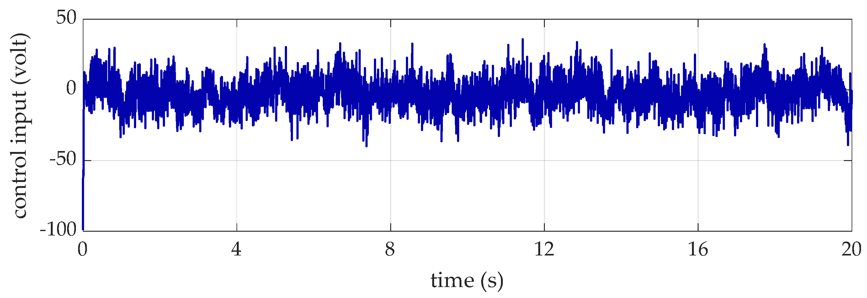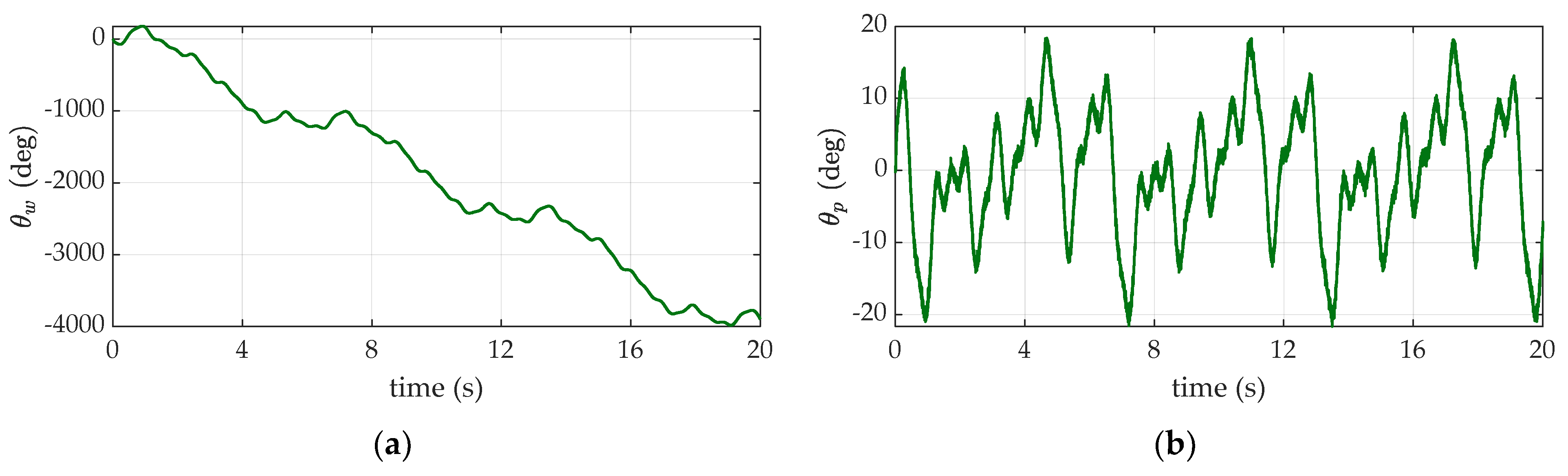Figure 2 illustrates the input signals used for closed-loop parameter identification under aggressive command excitation, while Figure 3 displays the corresponding system output responses. Apparently, due to the imperfection of the sensors, the input/output signals are contaminated by measurement noise. Therefore, the filter-based method becomes very important for noise suppression during the SPI, which has been highlighted in Table 1.

According to

Table 2. Parameter identification results with different excitation command input.

Reference Parameter	Simple Command		Aggressive Command
	Est. Para.	Error (%)	Est. Para.	Error (%)
$X_1=0.0436$	0.02921	33.04	0.04991	14.46
$X_2=0.0178$	0.03071	72.52	0.01276	28.26
$X_3=0.1149$	0.06709	41.60	0.10695	6.914
$X_4=0.8719$	0.51477	40.96	0.83680	4.027
$X_5=4.6701$	2.85297	38.91	4.67882	0.1025
$X_6=0.7268$	0.72685	0.0073	0.72695	0.0212
$X_7=0.7256$	0.72526	0.0474	0.70581	2.7282

, it is obvious that the parameters identified through the aggressive command are more accurate than the simple command. The results verify the assumption as mentioned before. In other words, an active command can excite wheel-driven pendulum cart’s dynamic response more obviously than just a simple command. Note that the selection of the filter time constants should not filter out the original system’s dynamic response, but should be able to suppress the measurement noise.

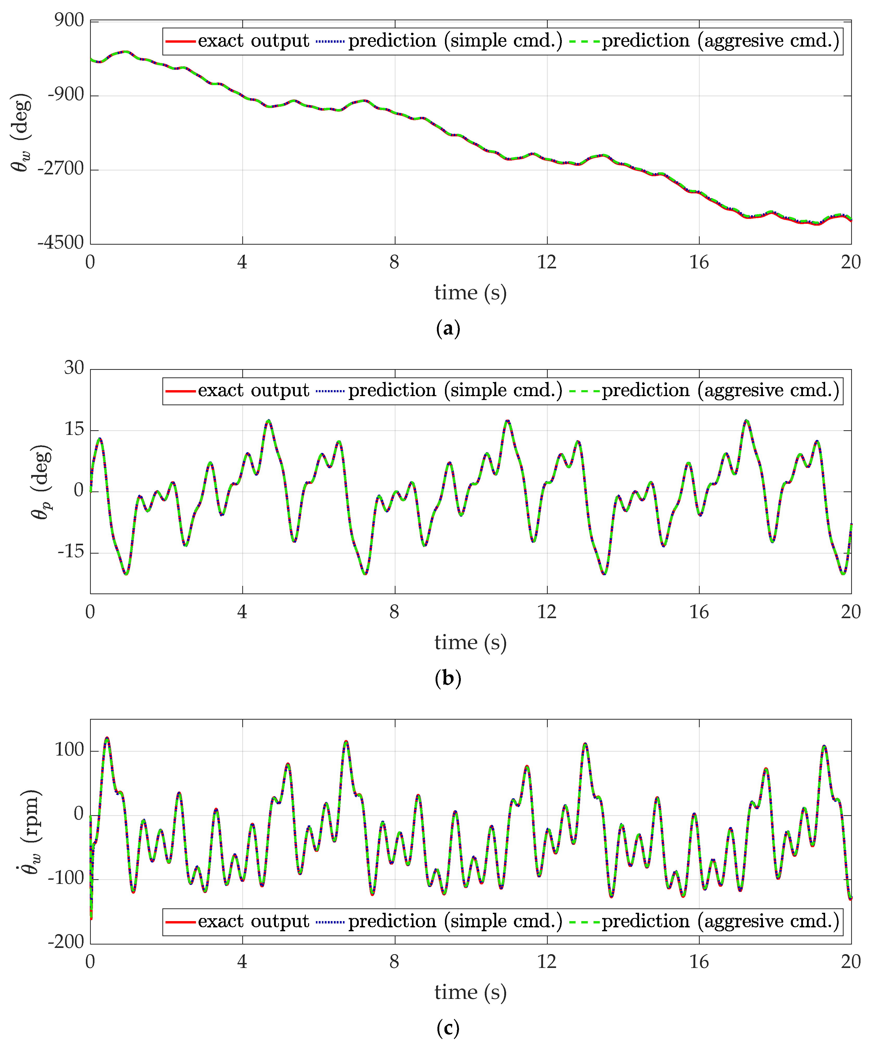
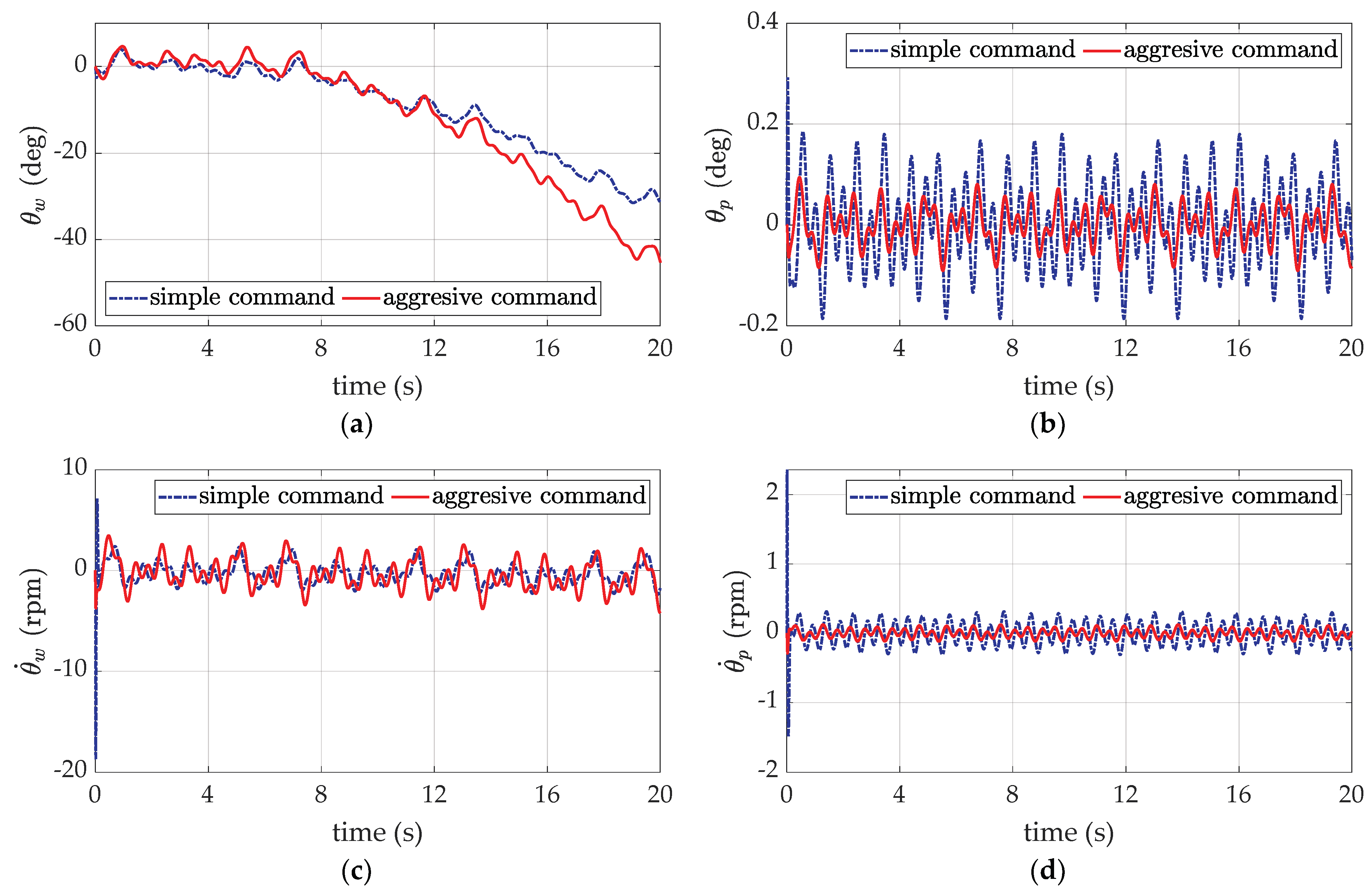
Based on the identified parameters, Figure 4 demonstrate the association output predictions. The red line represents the exact output response from true parameters. As for the blue and green line, the former stands for the prediction of parameters identified through simple command, while the latter is the prediction of parameters identified through aggressive command. One can observe that, from Figure 5, the RMSE (Root Mean Square Error) of the output prediction based on applying the identified parameters is very small. According to the simulation results, the RMSE for wheel angle output prediction is 0.3260 for the aggressive command and 0.2423 for the simple command, respectively. Besides, the RMSE for pitch angle output prediction is 6.8181e-04 for the aggressive command and 0.0016 for the simple command. Also, the RMSE for wheel angular rate output prediction is 0.1585 for the aggressive command and 0.1267 for the simple command. Lastly, the RMSE for pitch angular rate output prediction is 0.0064 for the aggressive command and 0.0201 for the simple command.

It is evident that states related to pitch, including pitch angle and pitch angular rate, exhibit lower output prediction errors when excited through an aggressive command compared to those excited by a simple command. In contrast, states associated with the wheel, although not showing significantly lower output prediction errors when excited through an aggressive command than when excited through a simple command, display very similar errors between the two cases.

This phenomenon can be attributed to the fact that the response of parameters identified through an aggressive command is superior to that of parameters identified through a simple command. The rationale behind this lies in the active command input’s capability to reduce the condition number of the observation matrix for the wheel-driven pendulum system. This reduction prevents the system from becoming ill-conditioned and thereby enhances the accuracy of parameter identification.

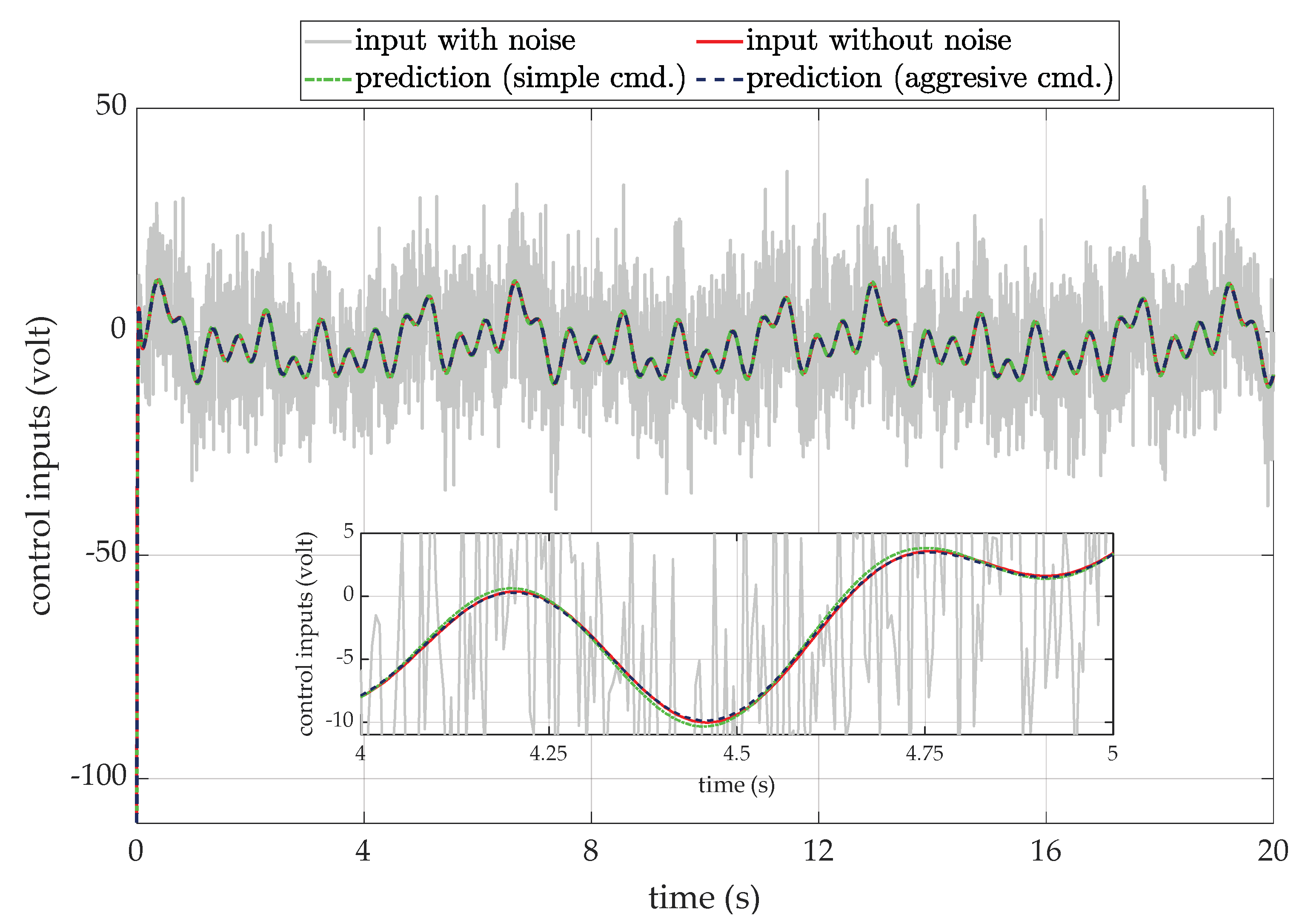
In the context of closed-loop system identification, the performance of system identification can be evaluated not only through the prediction of output responses but also by calculating the corresponding control inputs using the controller, thereby enabling control input predictions. Based on the results of closed-loop system identification, Figure 6 presents predictions of control inputs, comparing these predictions with both the measured and exact control inputs.

In Figure 6, the gray line represents the control input signal of the actual system with output measurement noise, the red line corresponds to the exact control input signal, while the green and blue lines represent the predicted control inputs obtained through the excitation of an simple command and an aggressive command, respectively. It is evident from the graph that the accuracy of control input prediction is influenced by the accuracy of pitch angle prediction, as control inputs are derived from the error between the reference command and the pitch angle. Consequently, the predictions generated through aggressive command excitation exhibit higher accuracy compared to those obtained through simple command excitation when compared to the exact control inputs.

When applying an output filtering method, it is necessary to perform numerical integration for specific system states as shown in (41), where the associated initial values for the integration is provided by (42). Consequently, any uncertainty in the initial value leading to bias results in the accumulation of errors in the system state over time, affecting the accuracy of the system state integration solution and, consequently, reducing the precision of parameter identification. Based on (42), it is evident that increasing the values of the filter parameters ${\tau }_1$ and ${\tau }_2$ can mitigate the impact of initial value uncertainty on numerical integration. To validate this statement, extra simulations are conducted to evaluate the accuracy of parameter identification under different cases. In order to clearly point out how the selection of the parameters ${\tau }_1$ and ${\tau }_2$ can affect the precision of the SPI, the following numerical cases are applied in the absence of output measurement noise. The results are summarized in

Table 3. The impact of various filter parameters on parameter identification results with initial value deviation.

Ref. Para.	Correct Initial Value		$\mathbf{Initial} \mathbf{Value} \mathbf{with} \mathbf{Uncertainty} ({\mathit{\theta }}_{\mathit{p}}$ Deviation Is +0.5 Degrees)
	$\mathbf{Case} \mathbf{A}. {\mathit{\tau }}_1 = {\mathit{\tau }}_2=0.014$		$\mathbf{Case} \mathbf{B}. {\mathit{\tau }}_1 = {\mathit{\tau }}_2 = 0.014$		$\mathbf{Case} \mathbf{C}. {\mathit{\tau }}_1={\mathit{\tau }}_2=0.14$		$\mathbf{Case} \mathbf{D}. {\mathit{\tau }}_1={\mathit{\tau }}_2=4.2$
	Est. Para.	Error (%)	Est. Para.	Error (%)	Est. Para.	Error (%)	Est. Para.	Error (%)
$X_1=0.0436$	0.04355	0.1074	0.00590	86.458	0.04033	7.4825	0.05016	15.053
$X_2=0.0178$	0.01781	0.0764	0.03485	95.787	0.01959	10.059	0.01248	29.844
$X_3=0.1149$	0.11475	0.1239	-0.00727	1.0633	0.10586	7.8629	0.12766	11.106
$X_4=0.8719$	0.87128	0.0707	-0.01024	1.0117	0.80374	7.8169	0.97554	11.886
$X_5=4.6701$	4.66554	0.0974	0.65966	85.874	4.34846	6.8870	5.24997	12.416
$X_6=0.7268$	0.72684	0.0061	0.72719	0.0546	0.72684	0.0064	0.72686	0.0084
$X_7=0.7256$	0.72516	0.0600	0.72203	0.4914	0.72592	0.0442	0.71614	1.3031

.

In this simulation comparison study, the controller parameters and initial system settings remain consistent with the previous simulations. As mentioned previously, the maximum system frequency of unstable systems is typically challenging to estimate beforehand. Therefore, the easiest way for the design of the filter parameters $\left({\tau }_1,{\tau }_2\right)$ is based on the system’s reference commands, see [10,11,18]. In Case A, serving as the ground truth, there is no initial value bias. Considering a cutoff frequency of the output filter that is 10 times the maximum reference command frequency, the filter parameters are designed with ${\tau }_1={\tau }_2=0.014$. In Case B, using the same filter parameters, the initial value uncertainty introduced by the IMU-based estimation of pitch angle is accounted for. Here, the initial value of the pitch angle bias is set to be with positive 0.5 degrees. Furthermore, to mitigate the effects of initial value uncertainty and assess the impact of increased filter parameters, we further conduct Case C, where filter parameters are adjusted to ${\tau }_1={\tau }_2=0.14$. To further discuss an inadequate selection of the parameters degrade the SPI precision, the Case D, where filter parameters are increased to ${\tau }_1={\tau }_2=4.2$, is demonstrated while keeping the same level of initial value uncertainty bias.

From Table 3, it can be observed that, as the ground truth in Case A, since there is no noise interference or initial value uncertainty, the filter-based SPI results in very low parameter estimation errors. However, under the influence of initial value bias in Case B, the accuracy of parameter identification is indeed affected, with some parameter estimation errors reaching up to 95%. To address the SPI error caused by initial value uncertainty, as shown in Case C, appropriately increasing the filter parameter values can effectively mitigate the impact of initial value uncertainty and reduce parameter estimation errors. Nevertheless, it should be emphasized that the filter parameter values cannot be infinitely increased, as previously discussed in the article. The concept of output filtering is based on the removal of noise from output data, and the physical significance of filter parameters is the cutoff frequency of the filter. Therefore, excessive increases in filter parameters may suppress the system’s dominant frequency response, making the original system behavior unobservable, which in turn decreases the accuracy of parameter estimation, as demonstrated in Case D.

In summary, when using the output filtering methods, the selection of the filter parameters carries significant implications. For unstable systems, under the condition of meeting basic tracking requirements, filter parameter design can be based on the maximum frequency of reference commands in the closed-loop control. The adjustment of filter parameters should not solely focus on noise removal, but should also consider the suppression of uncertainties in system initial value measurements.

Based on the above simulations, we can firmly conclude that the use of filtering-based system parameter identification can be applied to the nonlinear and unstable wheel-driven pendulum system successfully; the second-order output filtering method does not require the use of noisy acceleration signals, thus enabling more accurate parameter estimation; the filtering method is able to suppress the effects of Gaussian noise and quantization noise effectively; incorporation of aggressive command input can enhance the precision of parameter estimation.

Remark 1. 

In the process of system identification, unstable systems may lead to adverse experimental outcomes or even pose safety hazards. Therefore, utilizing closed-loop system identification not only ensures the stability during the SPI but also effectively estimates the parameters of unstable systems, subsequently reducing system uncertainties in later stages of control design. Furthermore, employing unstable systems for closed-loop model estimation as an application of digital twins holds significant value. Given the unique physical characteristics of unstable systems, arbitrary adjustments to system controller parameters may result in system divergence, or even more severe consequences such as system damage. Leveraging the concept of a digital twin, designers can perform preliminary assessments of physical systems within a virtual model and proceed with controller design. Through simulations, they can evaluate the expected performance of the controller, thus verifying the feasibility and effectiveness of the controller design. Ultimately, these designs can be applied to real-world systems, ensuring a safer and more reliable development of controllers prior to implementation and optimization.

5. Conclusions

This paper introduces an output filtering method to identify the system parameters of a nonlinear unstable wheel-driven pendulum cart. The detailed equations of motions and the associated measurement equations for the parameter identification are derived. Considering the real scenario, the measurement quantization as well as the Gaussian noises, which have a considerable impact on parameter estimations, are both taken into account. According to the presented filtering method, it cannot only suppress noisy acceleration, but preserve the dominant frequencies of the system’s response as well. Simulations firmly demonstrate that the presented output filtering method is superior to the direct numerical differentiation method. Furthermore, to excite the special dynamic response of the pendulum cart, a simple command and an aggressive command are applied to the system, respectively. Associated results show that the more active the reference command is, the more accurate the estimation results could be. In conclusion, precise system parameters can be obtained by applying the presented output filtering algorithm even in the presence of the measurement quantization effect as well as the measurement noise. Simulations are carried out to verify the feasibility of the purposed method.

References

1. Juang, J.-N.; Pappa, R.S. An eigensystem realization algorithm for modal parameter identification and model reduction. J. Guid. Control Dyn. 1985, 8, 620–627. [Google Scholar] [CrossRef]
2. Juang, J.-N. Applied System Identification; Prentice-Hall, Inc.: Hoboken, NJ, USA, 1994. [Google Scholar]
3. Juang, J.-N. Continuous-time bilinear system identification. Nonlinear Dyn. 2005, 39, 79–94. [Google Scholar] [CrossRef]
4. Juang, J.-N.; Phan, M.Q. Identification and Control of Mechanical Systems; Cambridge University Press: Cambridge, UK, 2001. [Google Scholar]
5. Jin, H.; Liu, Z.; Zhang, H.; Liu, Y.; Zhao, J. A dynamic parameter identification method for flexible joints based on adaptive control. IEEE/ASME Trans. Mechatron. 2018, 23, 2896–2908. [Google Scholar] [CrossRef]
6. Vicente, B.A.H.; James, S.S.; Anderson, S.R. Linear System Identification Versus Physical Modeling of Lateral–Longitudinal Vehicle Dynamics. IEEE Trans. Control Syst. Technol. 2021, 29, 1380–1387. [Google Scholar] [CrossRef]
7. Chan, R.P.M.; Stol, K.A.; Halkyard, C.R. Review of modelling and control of two-wheeled robots. Annu. Rev. Control 2013, 37, 89–103. [Google Scholar] [CrossRef]
8. Grasser, F.; D’arrigo, A.; Colombi, S.; Rufer, A.C. JOE: A mobile, inverted pendulum. IEEE Trans. Ind. Electron. 2002, 49, 107–114. [Google Scholar] [CrossRef]
9. Kim, H.; Jung, S. Control of a two-wheel robotic vehicle for personal transportation. Robotica 2016, 34, 1186–1208. [Google Scholar] [CrossRef]
10. Moreno-Valenzuela, J.; Miranda-Colorado, R.; Aguilar-Avelar, C. A matlab-based identification procedure applied to a two-degrees-of-freedom robot manipulator for engineering students. Int. J. Electr. Eng. Educ. 2017, 54, 319–340. [Google Scholar] [CrossRef]
11. Lopez-Sanchez, I.; Montoya-Cháirez, J.; Pérez-Alcocer, R.; Moreno-Valenzuela, J. Experimental Parameter Identifications of a Quadrotor by Using an Optimized Trajectory. IEEE Access 2020, 8, 167355–167370. [Google Scholar] [CrossRef]
12. Calanca, A.; Capisani, L.M.; Ferrara, A.; Magnani, L. MIMO Closed Loop Identification of an Industrial Robot. IEEE Trans. Control Syst. Technol. 2011, 19, 1214–1224. [Google Scholar] [CrossRef]
13. Jin, J.; Gans, N. Parameter identification for industrial robots with a fast and robust trajectory design approach. Robot. Comput.-Integr. Manuf. 2015, 31, 21–29. [Google Scholar] [CrossRef]
14. Peng, C.C.; Su, C.Y. Modeling and Parameter Identification of a Cooling Fan for Online Monitoring. IEEE Trans. Instrum. Meas. 2021, 70, 1–14. [Google Scholar] [CrossRef]
15. Moreno-Valenzuela, J.; Aguilar-Avelar, C. Motion Control of Underactuated Mechanical Systems; Springer: Berlin/Heidelberg, Germany, 2018; Volume 1. [Google Scholar]
16. Khalil, W.; Dombre, E. Modeling Identification and Control of Robots; CRC Press: Boca Raton, FL, USA, 2002. [Google Scholar]
17. Miranda-Colorado, R.; Moreno-Valenzuela, J. Experimental parameter identification of flexible joint robot manipulators. Robotica 2018, 36, 313–332. [Google Scholar] [CrossRef]
18. Chávez-Olivares, C.; Reyes-Cortés, F.; González-Galván, E.; Mendoza-Gutierrez, M.; Bonilla-Gutierrez, I. Experimental evaluation of parameter identification schemes on an anthropomorphic direct drive robot. Int. J. Adv. Robot. Syst. 2012, 9, 203. [Google Scholar] [CrossRef]
19. Guangjun, L.; Iagnemma, K.; Dubowsky, S.; Morel, G. A base force/torque sensor approach to robot manipulator inertial parameter estimation. In Proceedings of the 1998 IEEE International Conference on Robotics and Automation (Cat. No.98CH36146), Leuven, Belgium, 20–20 May 1998. [Google Scholar]
20. Guého, D.; Singla, P.; Majji, M.; Melton, R.G. Filtered Integral Formulation of the Sparse Model Identification Problem. J. Guid. Control Dyn. 2022, 45, 232–247. [Google Scholar] [CrossRef]
21. Peng, C.-C.; Chen, T.-Y. A recursive low-pass filtering method for a commercial cooling fan tray parameter online estimation with measurement noise. Measurement 2022, 205, 112193. [Google Scholar] [CrossRef]
22. Gautier, M.; Khalil, W.; Restrepo, P. Identification of the dynamic parameters of a closed loop robot. In Proceedings of the 1995 IEEE International Conference on Robotics and Automation, Nagoya, Japan, 21–27 May 1995. [Google Scholar]
23. Gautier, M. Dynamic identification of robots with power model. In Proceedings of the International Conference on Robotics and Automation, Albuquerque, NM, USA, 25 April 1997. [Google Scholar]
24. Li, Y.-R.; Peng, C.-C. Encoder position feedback based indirect integral method for motor parameter identification subject to asymmetric friction. Int. J. Non-Linear Mech. 2023, 152, 104386. [Google Scholar] [CrossRef]
25. Peng, C.-C.; Chen, Y.-H. A Hybrid Neural Ordinary Differential Equation Based Digital Twin Modeling and Online Diagnosis for an Industrial Cooling Fan. Future Internet 2023, 15, 302. [Google Scholar] [CrossRef]
26. Arvidsson, M.; Karlsson, J. Design, Construction and Verification of a Self-Balancing Vehicle. 2012. Available online: http://publications.lib.chalmers.se/records/fulltext/163640.pdf (accessed on 24 September 2023).
Figure 1. Cartesian coordinate of the wheel-driven cart schematic diagram, where red dot represents the center of mass of the cart.
Electronics 12 04569 g001
Figure 2. Input data for system identification.
Electronics 12 04569 g002
Figure 3. Output data for system identification. (a) Wheel angle. (b) Pitch angle. (c) Wheel angular speed. (d) Pitch angular speed.
Electronics 12 04569 g003aElectronics 12 04569 g003b
Figure 4. Outputs response predictions of the closed-loop model for the wheel-driven pendulum system. (a) Wheel angle. (b) Pitch angle. (c) Wheel angular speed. (d) Pitch angular speed.
Electronics 12 04569 g004aElectronics 12 04569 g004b
Figure 5. Outputs prediction errors of the closed-loop model. (a) Wheel angle. (b) Pitch angle. (c) Wheel angular speed. (d) Pitch angular speed.
Electronics 12 04569 g005
Figure 6. Control input prediction for closed-loop system.
Electronics 12 04569 g006