Robust Wind Power Ramp Control Strategy Considering Wind Power Uncertainty

Abstract

Recent climate change has worsened the risk of extreme weather events, among which extreme offshore wind storms threaten secure operation by inducing offshore wind power ramps. Offshore wind power ramps cause the instantaneous power fluctuation of interconnected onshore grids and may lead to unexpected load shedding or generator tripping. In this paper, considering offshore wind power uncertainties, we propose a novel robust coordinated offshore wind power ramp control strategy by dispatching thermal units, energy storage systems, and hydrogen storage systems cooperatively. First, the impact of extreme wind storms on an offshore wind farm output power ramp is analyzed, and the general framework of offshore wind power ramp control is presented based on the two-stage robust optimization considering the dual uncertainties of load demand and wind power. Second, a coordinated wind power ramp control model is established considering the operational characteristics of different ramp control sources such as thermal units, energy storage systems, and offshore wind farms. Third, a robust ramp control strategy is developed using the column-and-constraint generation (CC&G) algorithm. Simulation results show the effectiveness of the proposed ramp control strategy.

1. Introduction

Offshore wind power has attracted widespread attention for modern power systems, characterized by the high penetration of renewable power [1,2]. Nevertheless, climate change-driven wind storms frequently invade coastal areas, leading to more wind power fluctuation and ramp events. Wind power ramps can stress turbine components and lead to operational issues or even catastrophic failures. Besides, under the grid-connected mode, wind power ramp causes instantaneous power imbalance of the onshore grid, resulting in frequency instability and even unexpected load shedding or generator tripping. Therefore, it is essential to control offshore wind power ramps and enhance the secure operation of the onshore grid.

When injecting large-scale wind power into the power system, one of the main challenges is evaluating wind power variability [3]. Unlike conventional generation, wind power has unpredictability and high variability due to uncertain meteorological factors [4], posing challenges for power system energy management such as power planning, scheduling, and operation. Researchers have proposed various methods to quantify wind power uncertainties in energy management activities. Ref. [5] introduced the conditional range metric (CRM) to quantify short-term wind power variability. Ref. [6] further enhanced the accuracy and adaptability of the CRM-based method for sparsely sampled wind power time series using a gamma distribution model. Ref. [7] considered the quantification of wind power variability on various timescales. Taking wind resources in China as an example, ref. [8] assessed both temporal variability and spatial correlation. Ref. [9] studied the dependency between weather regimes and wind capacity variability. Rather than investigating the variability of wind power, some researchers considered the influence of wind power variability on system operation. Ref. [10] studied the impact of wind power variability on system operating reserves. Ref. [11] proposed robustness metrics to assess a wind farm’s ability to generate power with high mean value and low variability under changing wind conditions.

In order to alleviate the influence of wind power uncertainties on power system operation, researchers use scenario generation methods to generate multiple varying wind power scenarios to transform stochastic operational models into deterministic ones. Ref. [12] implemented scenario generation on the uncertain short-term wind power, which used the empirical cumulative distribution function to capture forecast error distribution and fluctuation distribution. Ref. [13] used a Gaussian mixture model to develop analytical conditional distributions for forecast errors in multiple wind farms and to generate scenarios from the non-Gaussian interdependent conditional distributions. Ref. [14] introduced a data-driven scenario generation approach based on generative adversarial networks, which effectively captured the temporal and spatial patterns of renewable energy production for multiple correlated resources, offering scalability compared with traditional probabilistic models. Ref. [15] developed an analytical generalized Gaussian mixture model to fit the probability distributions of different wind ramping features.

Besides wind ramp forecasting [16], wind ramp control considering uncertainties is attracting increased attention for the secure operation of power systems. A scenario-generation-based dispatch strategy considering wind power uncertainties requires the probabilistic distribution of uncertainty parameters (e.g., wind power prediction errors), which may not be accessible in real-world applications. Therefore, researchers use robust optimization (RO) to handle uncertainties [17,18,19]. RO requires less knowledge of the wind power uncertainty parameters and can be solved more efficiently [20]. Ref. [21] utilized adaptive RO to achieve the economic dispatch considering a significant integration of wind power. Ref. [22] presented an RO-based unit commitment model considering uncertain wind power generation. Ref. [23] employed a distributionally RO to achieve economic scheduling considering wind power uncertainties. Ref. [24] developed a novel recourse-cost constrained adaptive robust optimization model that incorporates binary recourse variables and considers both nominal and worst-case scenarios.

Energy storage systems (ESSs) can store extra wind power in wind power ramp events [25]. Hence, ESSs and wind farms often form a coalition and collectively offer smooth power with less wind power fluctuation. Unlike conventional electrochemical ESSs, the recent popular hydrogen storage systems have benefits such as a high energy density, long-term storage, and reduced greenhouse gas emissions. In wind power ramp events, the electrolyzer converts surplus power from wind power ramps into hydrogen, making profits in hydrogen markets to reduce control cost. Wind power ramp control is a special type of microgrid energy management activity. Previous microgrid energy management seldom considers how to design a cooperative ramp control strategy using electrochemical ESSs, HSSs, and conventional generators considering dual uncertainties of wind power and load demand. Therefore, a novel multi-source ramp control strategy is presented. First, we provide the problem formulation by expanding on the wind power ramp causes and necessity of ramp control. Second, we develop the multi-source cooperative ramp control framework based on two-stage RO. Third, we present the operational characteristics of ramp control sources such as the conventional generators, electrochemical ESSs, and hydrogen storage systems (HSSs). Fourth, we use the column-and-constraint generation algorithm (CC&G) to obtain the robust ramp control strategy, which is essentially a form of robust optimization strategy. The main contributions include the following:

• Considering the dual uncertainties of wind power and load demand, a two-stage robust optimization-based wind power ramp control framework is developed for multiple ramp control sources, such as conventional generators, electrochemical ESSs, and HSSs.
• A novel coordinated wind power ramp control strategy is proposed using the column-and-constraint generation (CC&G) algorithm. The proposed ramp control strategy can effectively handle the worse wind power ramp conditions with an enhanced economic performance by making extra profit in the hydrogen market.

The remainder of the paper is as follows: Section 2 provides the general framework of multi-source offshore wind power ramp control considering dual uncertainties of wind power and load demands; Section 3 presents the details of robust coordinated offshore wind power ramp control model and the corresponding robust ramp control strategy; Section 4 provides the formal analyses based on case study results; and Section 5 provides the concluding remarks.

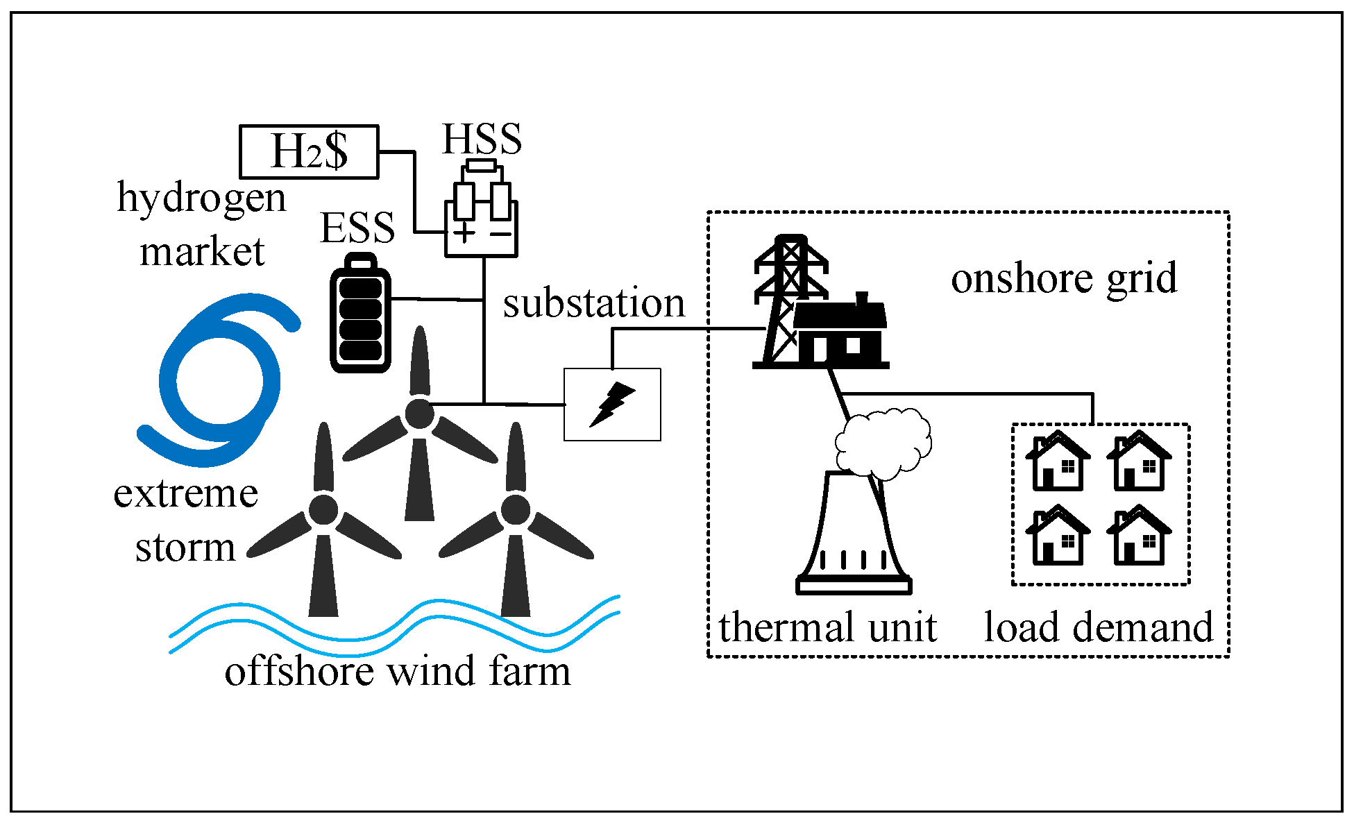
2. General Framework of Multi-Source Offshore Wind Power Ramp Control Considering Uncertainties

2.1. Wind Power Ramps and Impacts on Onshore Grid

Extreme storms usually have strong winds with fast wind speeds, which is one of the determining factors for wind power evaluation. Supposing that all of the wind turbines in the offshore wind farm are identical and the spatial differences among different wind turbines are neglected, the relation between the offshore wind power and the wind speed can be expressed by the piece-wise function-based power curve of an equivalent agglomerated wind turbine [26]:

$$P^{\mathrm{w}}\left(v\right)=\left\{\begin{array}{c}0v<v_{min}\hfill \\ P_{\mathrm{rated}}(z-yv+x{v}^2)v_{min}\le v\le v_{\mathrm{rated}}\hfill \\ P_{\mathrm{rated}}{v}_{\mathrm{rated}}\le v\le v_{max}\hfill \\ 0v>v_{max}\hfill \end{array}\right.$$

(1)

where v represents the wind speed, and $v_{min}$, $v_{\mathrm{rated}}$, and $v_{max}$ represent the cut-in wind speed, the rated wind speed, and the cut-out wind speed, respectively. x, y, and z are the power coefficients that depend on the characteristics of specific wind turbines. $P_{\mathrm{rated}}$ is the rated power of the wind turbine. If the wind speed falls below $v_{min}$ or beyond $v_{max}$, there will be no offshore wind power.

From the wind power curve in (1), we can see that as the wind speed increases, the wind power $P^{\mathrm{w}}\left(v\right)$ transitions from a small value to large one before reaching the saturation point $v_{min}\le v\le v_{\mathrm{rated}}$, and returns to zero after the wind speed hits the cut-out wind speed. During wind storm events, offshore wind farms experience sudden wind speed change, leading to an abrupt wind power change. Based on the wind curve in Formula (1), we can summarize the following wind power ramping events:

• Wind power ramp-up: when the wind speed v increases but remains below the cut-out wind speed $v_{max}$ over time $\Delta t$, if the magnitude of power change $\Delta P^{\mathrm{w}}$ exceeds the threshold $P_{\epsilon }$, based on the ramp definition in [27,28], it is recognized as a wind power ramp up event:

  $$\Delta P^{\mathrm{w}}=P_{t+\Delta t}^{\mathrm{w}}-P_t^{\mathrm{w}}>\Delta P_{\epsilon }$$

  (2)
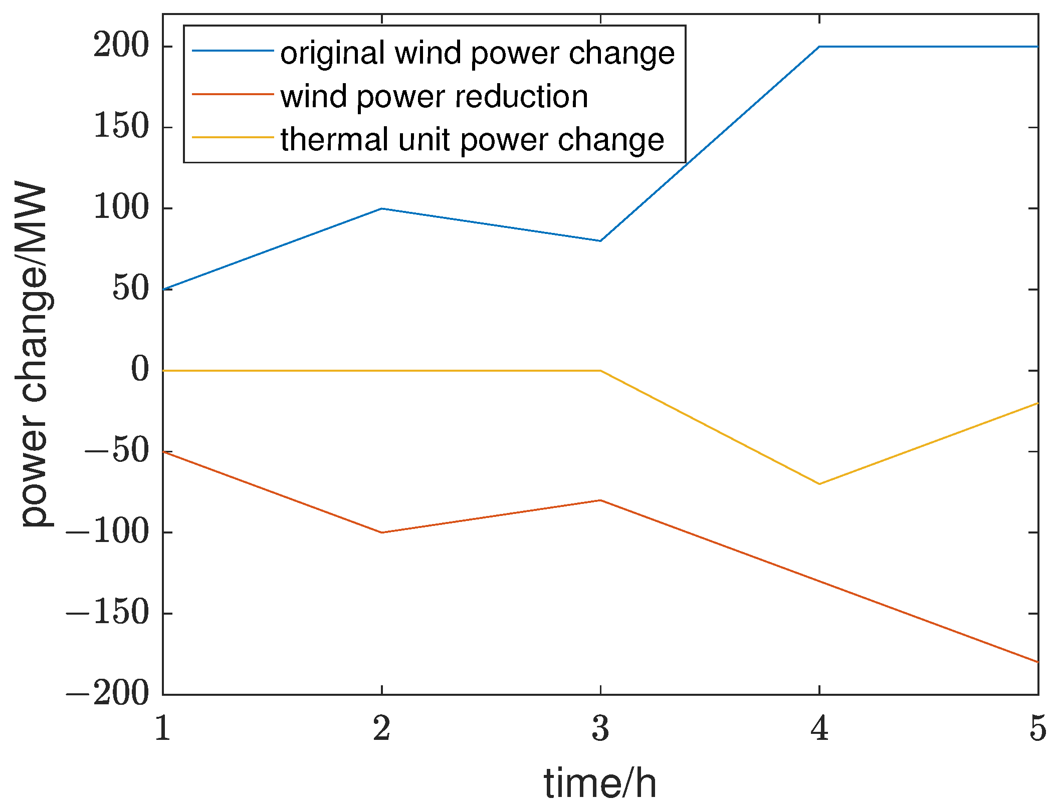
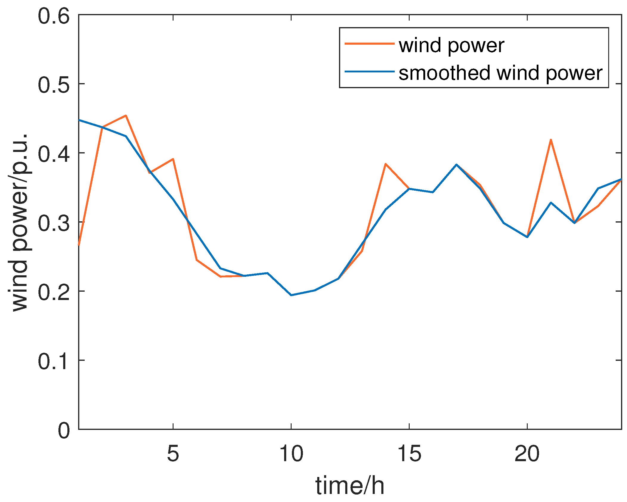
• Wind power ramp-down: when the wind speed v exceeds the cut-out speed $v_{max}$ over time $\Delta t$, the wind turbines collectively shut down and result in a significant decrease in the output power of the wind farm. If the magnitude of the power variation $\Delta P^{\mathrm{w}}$ exceeds the threshold $-P_{\epsilon }$ [27,28], a wind power ramp down event occurs:

  $$\Delta P^{\mathrm{w}}=P_{t+\Delta t}^{\mathrm{w}}-P_t^{\mathrm{w}}<-\Delta P_{\epsilon }$$

  (3)

When we operate an offshore wind farm in grid-connected mode, wind power ramps can cause an abrupt power imbalance in the onshore grid, threatening system security. We demonstrate the impact of offshore wind power ramps on the onshore grid using a simple test system containing one offshore wind farm and one thermal unit. Figure 1 provides the power change profiles of the thermal units and offshore wind farm.

Initially, the interconnected system achieves the power balance by satisfying $P_0^{\mathrm{w}}+P_{\mathrm{g}0}=P_{\mathrm{d}0}$. For the convenience of analysis, we assume that the load demands remain constant, i.e., $\Delta P_{\mathrm{d}}=0$. As is shown in Figure 1, from 1 h to 5 h, the wind farm output power fluctuates by 50 MW, 100 MW, 80 MW, 200 MW, and 200 MW, respectively. From 1 h to 3 h, the wind power ramp (i.e., 50 MW, 50 MW, and −20 MW) is no bigger than the ramp limit 50 MW of the thermal unit; hence, the thermal unit power changes by −50 MW, −100 MW, and −80 MW to guarantee the power balance $\Delta P\mathrm{w}+\Delta P_{\mathrm{g}}=\Delta P_{\mathrm{d}}=0$. Nevertheless, from 4 h to 5 h, the wind power ramp 120 MW surpasses the ramp limit 50 MW of the thermal unit; hence, even if the thermal unit reduces the power with a ramp limit of 50 MW, a power surplus of 70 MW and 20 MW at 4 h and 5 h, respectively, still exists. Therefore, the wind power reduction is 70 MW and 20 MW to rebalance the power. Meanwhile, the wind power reduction can control the wind power ramp from the original $\Delta P\mathrm{w}=120$ MW to the smoothed $\Delta P\mathrm{w}=50$ MW. In practice, wind power ramp control is more challenging for the following reasons:

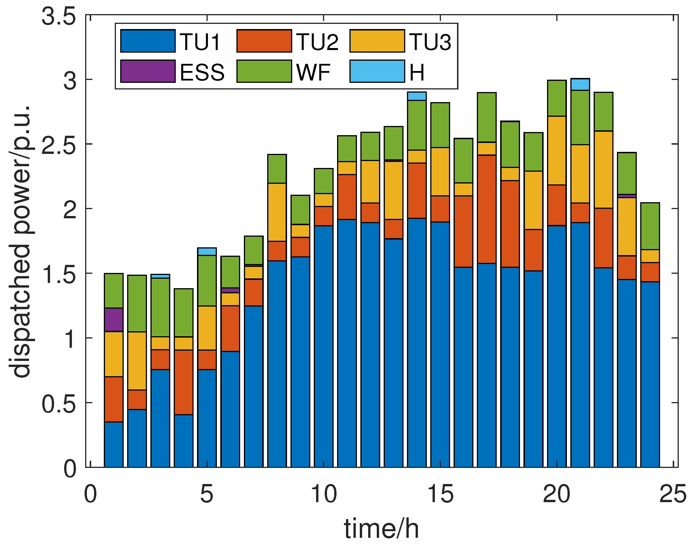
• the coordination of multiple ramp control sources: Unlike the simple system, the practical onshore grid usually contains multiple ramp control sources such as thermal units, electrochemical ESSs, and HSSs. Each ramp control resource has its unique operational characteristics such as generation limits, ramp limits, and expenses. Hence, it is challenging to dispatch these ramp control sources cooperatively to achieve specific goals.
• the impact of uncertainties: Unlike the one-line load demand or wind power profile. The practical wind power or load demand is usually uncertain, and the profile is in the form of strip rather the single line. Uncertainties in wind power or load demand make the ramp control more challenging because we need to obtain a deterministic dispatch strategy for all participating resources under uncertainties.

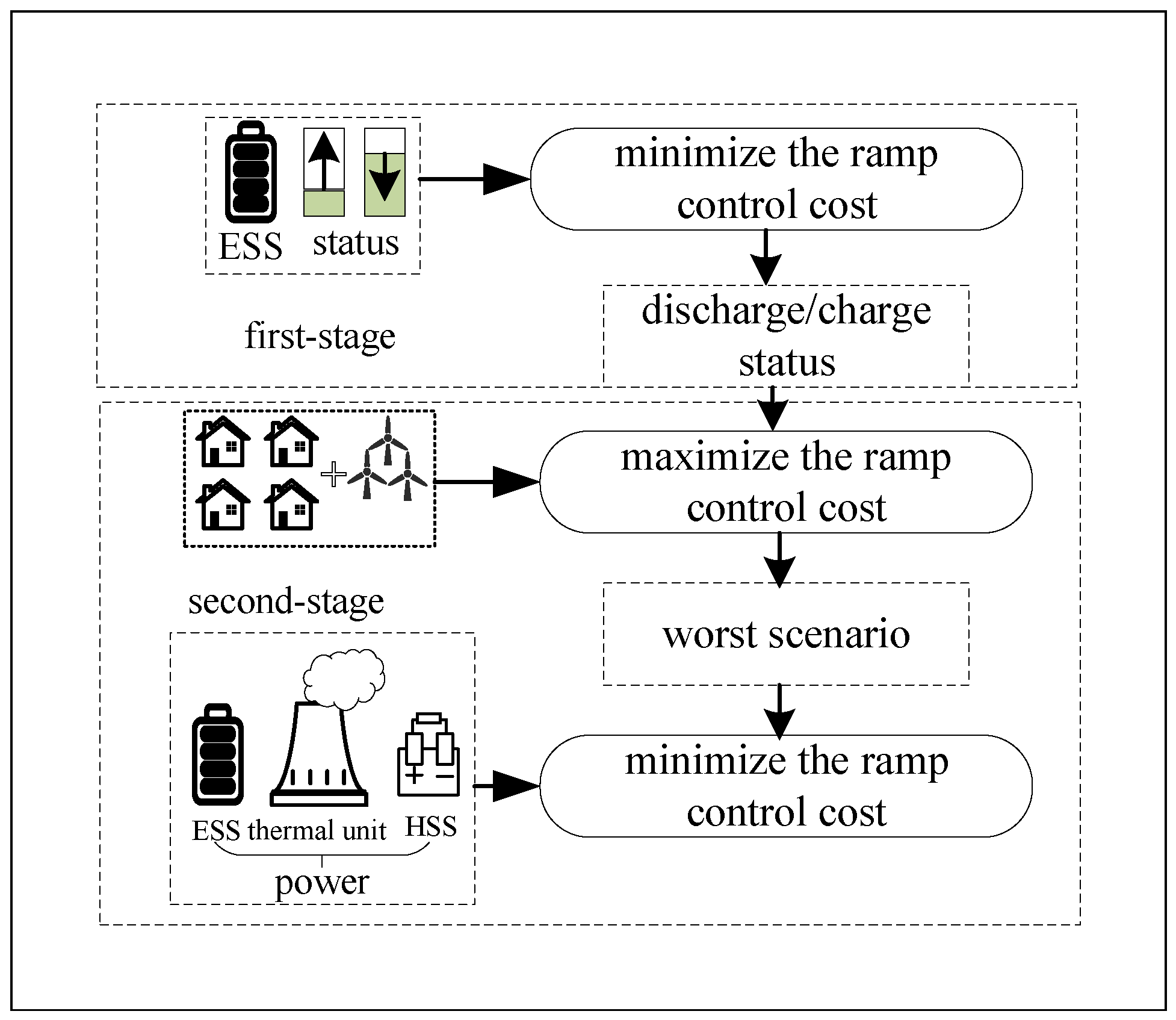
2.2. General Framework of Multi-Source Offshore Wind Power Ramp Control

In this section, considering the two challenges in Section 2.1, we provide the general framework of multi-source offshore wind power ramp control. The schematic diagram of the studied system is provided in Figure 2. The offshore wind farm injects wind power into the onshore grid. Meanwhile, the offshore wind farm converts a portion of wind power into hydrogen and trades in the hydrogen market. The onshore grid contains supplementary wind ramp control sources such as thermal units and ESSs. Based on the studied system in Figure 2, we present the ramp control framework. The proposed framework is based on the two-stage RO method. Mathematically, the framework can be written by a tri-level programming model:

$$\underset{u_{\mathrm{x}}}{min}\underset{u_{\mathrm{y}}}{max}\underset{u_{\mathrm{z}}}{min}\left(C_{\mathrm{g}}+C_{\mathrm{E}}-R_{\mathrm{h}}\right)$$

(4)

where $u_{\mathrm{x}}$ represents the first-stage decision variable such as the discharge/charge status of electrochemical ESSs; $u_{\mathrm{y}}$ represents the uncertainties such as the wind power and load demand; and $u_{\mathrm{z}}$ represents second-stage decision variables such as the discharge/charge power of electrochemical ESSs, the thermal unit power, and the converted wind power for hydrogen production. The objectives include the operational cost of thermal units $C_{\mathrm{g}}$, the operational cost of electrochemical ESSs $C_{\mathrm{E}}$, and the revenue from selling hydrogen $R_{\mathrm{h}}$. The inner layer shows that the ramp control center aims at minimizing the total costs minus the revenue. Unlike stochastic programming, which generates multiple scenarios, RO only considers the worst scenario. Hence, the middle layer uses the MAX operator to obtain the worst scenario from the uncertainty set. Unlike stochastic programming, which usually requires the scenario generation, $u_{\mathrm{y}}$ is usually expressed by an uncertainty set with known boundaries. The outer layer has a similar working principle as the inner layer; the main difference is the choice of decision variables. The first-stage decision variable $u_{\mathrm{x}}$ is implemented before the second-stage decision variable $u_{\mathrm{y}}$. Take electrochemical ESSs as an example, the discharge/charge status is predetermined. After obtaining the status, electrochemical ESSs, the discharge/charge power is calculated. Equation (4) provides the min–max–min-based objective function for the ramp control framework. Besides, each layer should satisfy certain constraints:

$$F\left(u_{\mathrm{x}},\varsigma \right)\le 0,u_{\mathrm{x}}\in S_{\mathrm{x}}$$

(5)

$$G\left(u_{\mathrm{x}},u_{\mathrm{y}},u_{\mathrm{z}},\varsigma \right)\le 0,u_{\mathrm{x}}\in S_{\mathrm{x}},u_{\mathrm{y}}\in S_{\mathrm{y}}$$

(6)

where $F(·)$ corresponds to the outer layer constraint and $G(·)$ corresponds to the inner layer constraint. As the middle layer decision variable $u_{\mathrm{y}}$ is an uncertainty set (e.g., a discrete set or a polyhedron), Equation (6) incorporates both the middle layer and inner layer decision variables. $\varsigma$ represents the operational states of the system and ramp control sources. From (4) to (6), we can see that the control center decides the first-stage and second-stage decision variables, sequentially considering the worst scenario, such that the ramp control cost is minimized. The strategy under the worst scenario has robustness under other uncertain scenarios to guarantee the secure operation under different levels of uncertainties. The schematic diagram of the two-stage RO-based ramp control framework is provided in Figure 3. After obtaining the optimal power schedule, the dispatch center sends the optimal power order to the respective regulation source, including thermal units and ESSs. As for asynchronous machines such as ESSs, converter-cell power of ESS will track the optimal power order using the active power control system of converter cells [29,30,31,32].

3. Robust Coordinated Offshore Wind Power Ramp Control Model and Strategy

Based on the proposed ramp control framework (4)–(6), this section first provides details of the robust coordinated offshore wind power ramp control model; second, the corresponding robust strategy is established using the column-and-constraint generation (CC&G) algorithm.

3.1. Coordinated Wind Power Ramp Control Model

The operational characteristics of ramp control sources are provided as follows:

3.1.1. Electrochemical Energy Storage System

The operational constraints of electrochemical ESSs are written by:

$$0\le P_{j,t}^{\mathrm{dis}}\le u_{j,t}^{\mathrm{dis}}{P}_j^{\mathrm{dis},\max },\forall t\in {\mathcal{N}}_{\mathrm{T}},\forall j\in {\mathcal{N}}_{\mathrm{s}}$$

(7)

$$0\le P_{j,t}^{\mathrm{ch}}\le u_{j,t}^{\mathrm{ch}}{P}_j^{\mathrm{ch},\max },\forall t\in {\mathcal{N}}_{\mathrm{T}},\forall j\in {\mathcal{N}}_{\mathrm{s}}$$

(8)

$$u_{j,t}^{\mathrm{dis}}+u_{j,t}^{\mathrm{ch}}\le 1,\forall t\in {\mathcal{N}}_{\mathrm{T}},\forall j\in {\mathcal{N}}_{\mathrm{s}}$$

(9)

$$S_j^{min}\le S_{j,t}\le S_j^{max}$$

(10)

$$S_{j,t}=S_{j,t-1}-P_{j,t}^{\mathrm{dis}}/{\eta }_j^{\mathrm{dis}}+P_{j,t}^{\mathrm{ch}}{\eta }_j^{\mathrm{ch}},\forall t\in {\mathcal{N}}_{\mathrm{T}},\forall j\in {\mathcal{N}}_{\mathrm{s}}$$

(11)

$$S_{j,\mathrm{T}}=S_{j,\mathrm{fin}},S_{j,0}=S_{j,\mathrm{ini}}\forall j\in {\mathcal{N}}_{\mathrm{s}}$$

(12)

where $P_j^{\mathrm{dis},\max }$ and $P_j^{\mathrm{ch},\max }$ represent the limits of discharge and charge power the ESS j, respectively, and $P_{j,t}^{\mathrm{ch}}$ and $P_{j,t}^{\mathrm{dis}}$ represent the charge and discharge power of ESS j at time t, respectively. $S_{j,t}$ represents the battery state of charge (SoC) of ESS j at time t. $u_{j,t}^{\mathrm{ch}}$ and $u_{j,t}^{\mathrm{dis}}$ represent the charge and discharge status of ESS j at time t, respectively; $S_j^{min}$ and $S_j^{max}$ denote the minimum and maximum capacity of the ESS j, respectively; ${\eta }_j^{\mathrm{dis}}$ and ${\eta }_j^{\mathrm{ch}}$ are the discharge and charge efficiency of the energy storage j, respectively; and $S_{j,\mathrm{ini}}$ and $S_{j,\mathrm{fin}}$ are the initial and final SoC, respectively.

Equations (7) and (8) require that the discharge or charge power cannot surpass the maximum or minimum discharge or charge power. Equation (9) requires that the ESS cannot simultaneously discharge or charge power. Equation (10) requires that SoC of ESS j at time t can surpass its minimum or maximum capacity. Equation (11) gives the relation between the SoC at time t and that at time $t-1$. Equation (12) gives the initial and final SoC during the ramp control interval.

3.1.2. Offshore Wind Farm and Hydrogen Storage System

Based on Figure 2, the hydrogen storage system is one component of the offshore wind farm; hence this section provides the combined wind farm and HSS model.

The offshore wind farm can convert a portion of wind power into hydrogen and curtail a portion of wind power. Both can attenuate the wind power ramp.

$${\overline{P}}_{j,t}^{\mathrm{w}}=P_{j,t}^{\mathrm{w}}-P_{j,t}^{\mathrm{wh}}+P_{j,t}^{\mathrm{dis}}-P_{j,t}^{\mathrm{ch}},\forall t\in {\mathcal{N}}_{\mathrm{T}},\forall j\in {\mathcal{N}}_{\mathrm{w}}$$

(13)

where $P_{j,t}^{\mathrm{w}}$ is the original wind power of wind farm j at time t; $P_{j,t}^{\mathrm{wh}}$ is the wind power that is converted to hydrogen; ad ${\overline{P}}_{j,t}^{\mathrm{w}}$ is the wind power after ramp control.

Besides, the wind farm output power under ramp control should satisfy the ramp requirement:

$$P_j^{\mathrm{w},\mathrm{dn}}\le {\overline{P}}_{j,t}^{\mathrm{w}}-{\overline{P}}_{j,t-1}^{\mathrm{w}}\le P_j^{\mathrm{w},\mathrm{up}},t\in {\mathcal{N}}_{\mathrm{T}}\backslash 1,\forall j\in {\mathcal{N}}_{\mathrm{w}}$$

(14)

where ${\overline{P}}_{j,t}^{\mathrm{w}}$ represents the smoothed wind power of wind farm j at t; $P_j^{\mathrm{w},\mathrm{dn}}$ and $P_j^{\mathrm{w},\mathrm{up}}$ represent the ramp-down and ramp-up limits of wind farm j, respectively.

$$P_j^{\mathrm{w},\mathrm{dn}}\le {\overline{P}}_{j,1}^{\mathrm{w}}-{\overline{P}}_{j,0}^{\mathrm{w}}\le P_j^{\mathrm{w},\mathrm{up}},t=1,\forall j\in {\mathcal{N}}_{\mathrm{w}}$$

(15)

where ${\overline{P}}_{j,0}^{\mathrm{w}}$ represents the initial wind power.

The relation between hydrogen production $H_{j,t}$ and wind power consumption $P_{j,t}^{\mathrm{wh}}$ is provided by the following:

$$H_{j,t}={\eta }_e\left(P_{j,t}^{\mathrm{wh}}\right)P_{j,t}^{\mathrm{wh}},t\in {\mathcal{N}}_{\mathrm{T}},\forall j\in {\mathcal{N}}_{\mathrm{w}}$$

(16)

where ${\eta }_e(·)$ represents the conversion efficiency of the electrozyer, which is affected by the consumed wind power $P_{j,t}^{\mathrm{wh}}$.

Considering the hydrogen load requirements, the stored hydrogen should satisfy the boundary constraint:

$$L_{\mathrm{H},\min }\le {\sum }_t{\sum }_j{H}_{j,t}\le L_{\mathrm{H},\max },t\in {\mathcal{N}}_{\mathrm{T}},\forall j\in {\mathcal{N}}_{\mathrm{w}}$$

(17)

where $L_{\mathrm{H},\min }$ and $L_{\mathrm{H},\max }$ represent the minimum and maximum hydrogen demand, respectively.

3.1.3. Thermal Unit

Thermal units on the onshore grid mainly support the load demand, and the generation limits are expressed by:

$$P_j^{\mathrm{g},min}\le P_{j,t}^{\mathrm{g}}\le P_j^{\mathrm{g},max},t\in {\mathcal{N}}_{\mathrm{T}},\forall j\in {\mathcal{N}}_{\mathrm{g}}$$

(18)

where $P_j^{\mathrm{g},min}$ represents the minimum generation capacity of thermal unit j and $P_j^{\mathrm{g},max}$ represents the maximum generation capacity of thermal unit j. The ramp limits are expressed by the following:

$$P_j^{\mathrm{g},\mathrm{dn}}\le P_{j,t}^{\mathrm{g}}-P_{j,t-1}^{\mathrm{g}}\le P_j^{\mathrm{g},\mathrm{up}},t\in {\mathcal{N}}_{\mathrm{T}}\backslash 1,\forall j\in {\mathcal{N}}_{\mathrm{g}}$$

(19)

where $P_j^{\mathrm{g},\mathrm{dn}}$ represents the ramp-down limit of thermal unit j and $P_j^{\mathrm{g},\mathrm{up}}$ represents the ramp-up limit of thermal unit j.

$$P_j^{\mathrm{g},\mathrm{dn}}\le P_{j,1}^{\mathrm{g}}-P_{j,0}^{\mathrm{g}}\le P_j^{\mathrm{g},\mathrm{up}},t=1,\forall j\in {\mathcal{N}}_{\mathrm{g}}$$

(20)

where $P_{j,0}^{\mathrm{g}}$ represents the initial power of the thermal unit j.

3.1.4. Uncertainty Model

As is described in (4)–(6), uncertainties play an important role in determining the role of the two-stage RO-based min–max–min model. This section provides a mathematical definition of both wind power and load uncertainties.

The relation between the actually used wind power $P_{j,t}^{\mathrm{w}}$ and the predicted power $P_{j,t}^{\mathrm{w},\mathrm{pre}}$ can be written by the following:

$$P_{j,t}^{\mathrm{w}}=P_{j,t}^{\mathrm{w},\mathrm{pre}}-{\delta }_{\mathrm{w}}{\mu }_{j,t}^{\mathrm{w}},t\in {\mathcal{N}}_{\mathrm{T}},\forall j\in {\mathcal{N}}_{\mathrm{w}}$$

(21)

where ${\delta }_{\mathrm{w}}$ represents the variation coefficient of wind power; ${\mu }_{j,t}^{\mathrm{w}}$ represents the variation status. The overall variation status along the control horizon satisfies the following:

$${\sum }_t{\mu }_{j,t}^{\mathrm{w}}\le {\Gamma }_j^{\mathrm{w}}$$

(22)

where ${\Gamma }_j^{\mathrm{w}}$ represents the maximal volatility degree of wind power. Similarly, we can define the load uncertainties as follows:

$$P_{j,t}^{\mathrm{d}}=P_{j,t}^{\mathrm{d},\mathrm{pre}}-{\delta }_{\mathrm{d}}{\mu }_{j,t}^{\mathrm{d}},t\in {\mathcal{N}}_{\mathrm{T}},\forall j\in {\mathcal{N}}_{\mathrm{d}}$$

(23)

where ${\delta }_{\mathrm{d}}$ represents the variation coefficient of the load demand and ${\mu }_{j,t}^{\mathrm{d}}$ represents the variation status. The overall variation status along the control horizon satisfies:

$${\sum }_t{\mu }_{j,t}^{\mathrm{d}}\le {\Gamma }_j^{\mathrm{d}}$$

(24)

where ${\Gamma }_j^{\mathrm{d}}$ represents maximal volatility degree of the load demand. Besides the operational characteristics of the ramp control sources, the ramp control should satisfy system-level operational constraints.

3.1.5. Power Flow Constraints

This paper adopts DC power flow based on the power transfer distribution factor (PTDF). The relation between branch power flow and nodal injection power is written by:

$${\mathit{P}}_{\mathrm{line}}=\mathit{H}{\mathit{P}}_{\mathrm{inj}}$$

(25)

where ${\mathit{P}}_{\mathrm{line}}$ represents the branch power flow vector, ${\mathit{P}}_{\mathrm{inj}}$ represents the nodal injection power vector, and $\mathit{H}$ is the corresponding PTDF matrix.

$$P_l^{min}\le P_{l,t}\le P_l^{max},t\in {\mathcal{N}}_{\mathrm{T}},\forall j\in {\mathcal{N}}_{\mathrm{l}}$$

(26)

where $P_l^{min}$ and $P_l^{max}$ represent the minimum and maximum power flow of line l, respectively.

3.1.6. Power Balance Constraints

$${\sum }_i{P}_{i,t}^{\mathrm{g}}+{\sum }_k(P_{k,t}^{\mathrm{w}}-P_{k,t}^{\mathrm{h}})={\sum }_j{P}_{j,t}^{\mathrm{d}}+{\sum }_k(P_{k,t}^{\mathrm{ch}}-P_{sj,t}^{\mathrm{dis}}),\forall t\in T$$

(27)

3.1.7. Objective Function

The objective of wind ramp control is used to minimize the ramp control cost:

$$\underset{{\mathit{\mu }}^{\mathrm{dis}},{\mathit{\mu }}^{\mathrm{ch}}}{min}\underset{{\mathit{P}}^{\mathrm{w}},{\mathit{P}}^{\mathrm{d}}}{max}\underset{{\mathit{P}}^{\mathrm{g}},{\mathit{P}}^{\mathrm{dis}},{\mathit{P}}^{\mathrm{ch}}}{min}\left(C_{\mathrm{g}}\left({\mathit{P}}^{\mathrm{g}}\right)+C_{\mathrm{e}}\left({\mathit{P}}^{\mathrm{dis}},{\mathit{P}}^{\mathrm{ch}}\right)-F_{\mathrm{h}}\left(\mathrm{H}\right)\right)$$

(28)

where $C_{\mathrm{g}}(·)$ and $C_{\mathrm{e}}(·)$ represent the total cost function of the thermal units and ESSs, respectively.

$$C_{\mathrm{g}}\left({\mathit{P}}^{\mathrm{g}}\right)={\sum }_i{\sum }_t{C}_{\mathrm{g}}\left(P_{i,t}^{\mathrm{g}}\right)$$

(29)

$$C_{\mathrm{g}}\left(P_{i,t}^{\mathrm{g}}\right)=a_i{P_{i,t}^{\mathrm{g}}}^2+b_i{P}_{i,t}^{\mathrm{g}}+c_i$$

(30)

where $a_i$, $b_i$, and $c_i$ are the cost coefficients of thermal units.

$$C_{\mathrm{e}}\left({\mathit{P}}^{\mathrm{dis}},{\mathit{P}}^{\mathrm{ch}}\right)={\sum }_j{\sum }_t{C}_{\mathrm{e}}\left(P_{j,t}^{\mathrm{dis}},P_{j,t}^{\mathrm{ch}}\right)$$

(31)

$$C_{\mathrm{e}}\left(P_{j,t}^{\mathrm{dis}},P_{j,t}^{\mathrm{ch}}\right)={\beta }_j^{\mathrm{dis}}{P}_{j,t}^{\mathrm{dis}}-{\beta }_j^{\mathrm{ch}}{P}_{j,t}^{\mathrm{ch}}$$

(32)

where ${\beta }_j$ is the ESS cost coefficient.

3.2. Coordinated Wind Power Ramp Control Strategy

Based on the ramp control model in Section 3.1, the compact-form two-stage RO model can be expressed by:

$$\underset{{\mathit{u}}_{\mathrm{x}}}{min}\underset{{\mathit{u}}_{\mathrm{y}}\in \Omega }{max}\underset{{\mathit{u}}_{\mathrm{z}}\in f\left({\mathit{u}}_{\mathrm{x}},{\mathit{u}}_{\mathrm{y}}\right)}{min}{C}_{\mathrm{total}}$$

(33)

$${\mathit{u}}_{\mathrm{x}}=\left\{{\mu }_{j,t}^{\mathrm{dis}},{\mu }_{j,t}^{\mathrm{ch}}\right\}$$

(34)

$${\mathit{u}}_{\mathrm{y}}=\left\{P_{k,t}^{\mathrm{w}},P_{i,t}^{\mathrm{d}}\right\}$$

(35)

$${\mathit{u}}_{\mathrm{z}}=\left\{P_{i,t}^{\mathrm{g}},P_{j,t}^{\mathrm{dis}},P_{j,t}^{\mathrm{ch}}\right\}$$

(36)

$$C_{\mathrm{total}}=\left(C_{\mathrm{g}}\left({\mathit{P}}^{\mathrm{g}}\right)+C_{\mathrm{e}}\left({\mathit{P}}^{\mathrm{dis}},{\mathit{P}}^{\mathrm{ch}}\right)-F_{\mathrm{h}}\left(\mathrm{H}\right)\right)$$

(37)

where $\Omega$ is equal to (21)–(24), f is equal to (7)–(20). The operational constraints can be written in a compact form:

$$\left\{\begin{array}{c}\mathit{A}{\mathit{u}}_{\mathrm{z}}+\mathit{G}{\mathit{u}}_{\mathrm{y}}=0\hfill \\ \mathit{B}{\mathit{u}}_{\mathrm{z}}\ge \mathit{b}\hfill \\ \mathit{C}{\mathit{u}}_{\mathrm{z}}+\mathit{D}{\mathit{u}}_{\mathrm{x}}\ge 0\hfill \\ {\mathit{u}}_{\mathrm{y}}={\widehat{\mathit{u}}}_{\mathrm{y}}-\mathit{\delta }\mathit{\mu }\hfill \\ \mathit{E}\mathit{\mu }\le \mathit{e}\hfill \end{array}\right.$$

(38)

This paper adopts the CC&G algorithm to solve (33). Before providing the solution procedures, we first present the sub-problem and master-problem, respectively.

3.2.1. Sub-Problem of Ramp Control

The sub-problem is actually a bi-level max–min problem, which is NP-hard. In this case, Karush–Kuhn–Tucker (KKT) conditions were employed to transfrom the bi-level model into the single level model. The Lagrange function is written as follows:

$$\mathcal{L}=C_{\mathrm{total}}+{\mathit{\lambda }}_{\mathrm{eq}}\left(\mathit{A}{\mathit{u}}_{\mathrm{z}}+\mathit{G}{\overline{\mathit{u}}}_{\mathrm{y}}\right)+{\mathit{\lambda }}_{\mathrm{ineq}1}\left(\mathit{b}-\mathit{B}{\mathit{u}}_{\mathrm{z}}\right)+{\mathit{\lambda }}_{\mathrm{ineq}2}\left(-\mathit{C}{\mathit{u}}_{\mathrm{z}}-\mathit{D}{\overline{\mathit{u}}}_{\mathrm{x}}\right)$$

(39)

where ${\mathit{\lambda }}_{\mathrm{eq}}$, ${\mathit{\lambda }}_{\mathrm{ineq}1}$, and ${\mathit{\lambda }}_{\mathrm{ineq}2}$ represent the dual variables of the first three constraints in (38). The KKT conditions can be expressed by:

$$\left\{\begin{array}{c}0\le \left(\mathit{B}{\mathit{u}}_{\mathrm{z}}-\mathit{b}\right)\perp {\mathit{\lambda }}_{\mathrm{ineq}1}\ge 0\hfill \\ 0\le \left(\mathit{C}{\mathit{u}}_{\mathrm{z}}+\mathit{D}{\overline{\mathit{u}}}_{\mathrm{x}}\right)\perp {\mathit{\lambda }}_{\mathrm{ineq}2}\ge 0\hfill \\ \frac{\partial \mathcal{L}}{\partial {\mathit{u}}_{\mathrm{z}}}=0\hfill \end{array}\right.$$

(40)

Note that the KKT conditions contain nonlinear complementary slackness conditions; we can use the Big-M method to transform them into linear constraints.

3.2.2. Master-Problem of Ramp Control

The master problem is the first-stage problem, we define the second-stage decision variables of iteration m as ${\mathit{u}}_{\mathit{z},m}$.

$$\underset{{\mathit{u}}_{\mathit{x}}}{min}\alpha$$

(41)

$$\left\{\begin{array}{c}\alpha \ge C_{\mathrm{total}}\hfill \\ \mathit{A}{\mathit{u}}_{\mathrm{z},\mathrm{m}}+\mathit{G}{\mathit{u}}_{\mathrm{y}}=0\hfill \\ \mathit{B}{\mathit{u}}_{\mathrm{z},\mathrm{m}}\ge \mathit{b}\hfill \\ \mathit{C}{\mathit{u}}_{\mathrm{z},\mathrm{m}}+\mathit{D}{\mathit{u}}_{\mathrm{x}}\ge 0\hfill \end{array}\right.$$

(42)

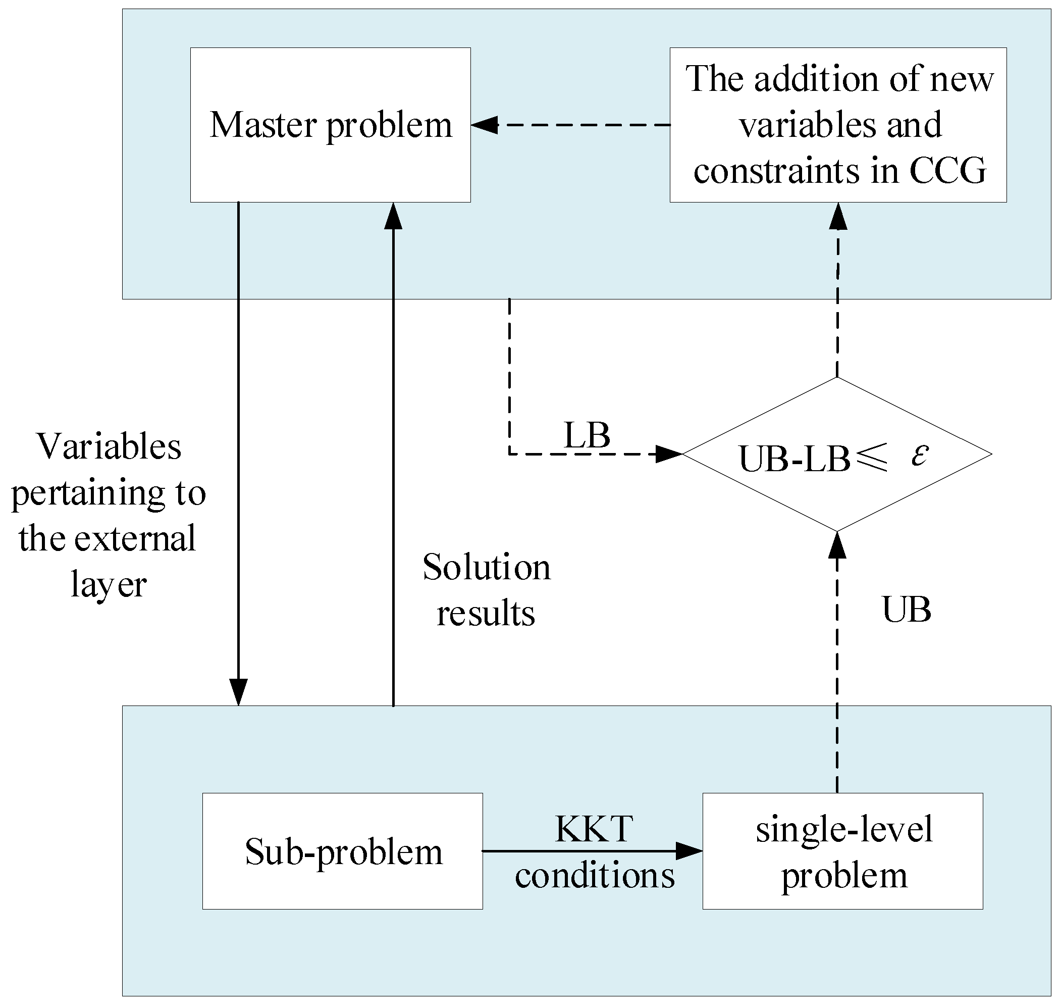
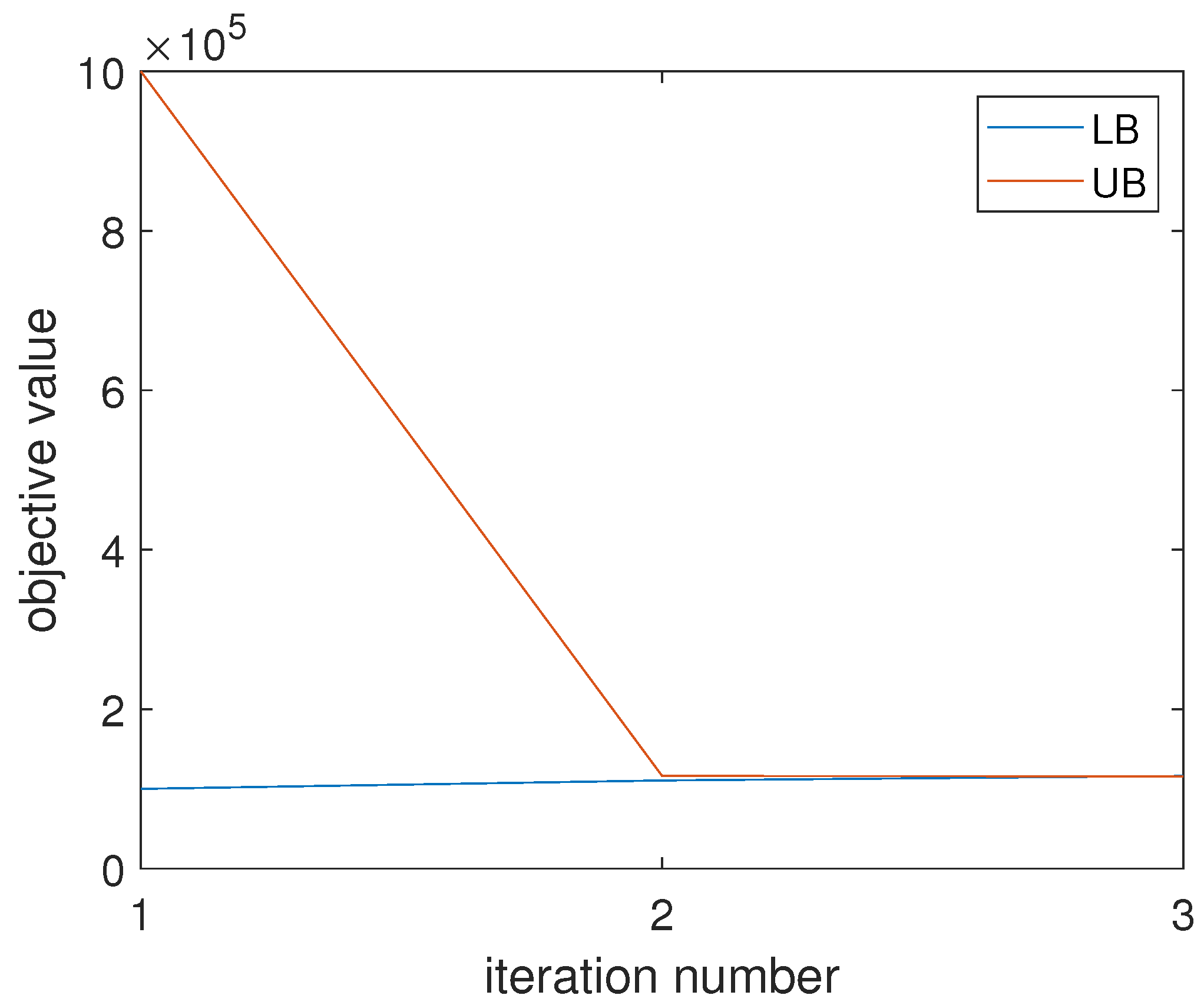
3.2.3. Column Constraint Generation-Based Robust Ramp Control Strategy

Based on the sub-problem and master-problem in Section 3.2.1 and Section 3.2.2, we provide the CC&G-based robust strategy computation procedures in Figure 4:

• Step 1: initialize the upper bound $UB=+\infty$ and lower bound $LB=-\infty$; the iteration number $m=1$; the maximum iteration number is $m_{\max }=100$. Initialize the worst scenario ${\mathit{u}}_{\mathrm{y},0}$.
• Step 2: compute the master-problem to obtain the ${\overline{\mathit{u}}}_{\mathrm{x}}$, and $C_{\mathrm{total},\mathrm{m}}$. Let $LB=C_{\mathrm{total},\mathrm{m}}$.
• Step 3: substitute ${\overline{\mathit{u}}}_{\mathrm{x}}$ into the sub-problem to obtain the $C_{\mathrm{total},\mathrm{s}}$ and the worst scenario ${\mathit{u}}_{\mathrm{y},\mathrm{m}}$. Let $UB=min(UB,C_{\mathrm{total},\mathrm{s}})$.
• Step 4: if $UB-LB\le ϵ$, output the strategy; otherwise, $m=m+1$, go to Step 2.

Figure 4. CC&G algorithm-based ramp control strategy flow chart.

Figure 4. CC&G algorithm-based ramp control strategy flow chart.

4. Case Studies

We used the standard IEEE 14-bus system for the case studies. Specifically, we placed the wind farm at bus 9 and the ESSs at bus 4. Load and wind power prediction can be found in PJM Data Miner [33].

Table 1. Parameters of the two-stage robust optimization model.

Unit	Parameter	Value
Energy storage	${\beta }_j^{\mathrm{dis}}/$ CHY/MWh	22
	${\beta }_j^{\mathrm{ch}}/$ CHY/MWh	20
	$R_{sj}^{\mathrm{dis}}/$ MW, $R_{sj}^{\mathrm{ch}}/$ MW	20
	$S_j^{min}/$ MW	6
	$S_j^{max}/$ MW	60
	$S_{j,\mathrm{fin}}/$ MW	50
	$S_{j,\mathrm{ini}}/$ MW	20
	${\eta }_j^{\mathrm{dis}}$, ${\eta }_j^{\mathrm{ch}}$	0.9
Wind turbine	$P_j^{\mathrm{w},\mathrm{dn}}$, $P_j^{\mathrm{w},\mathrm{up}}/$ MW	5

gives the key prarameter information.

In order to simulate the uncertainties of wind power and load demand, the uncertainty factors were ${\Gamma }_j^{\mathrm{d}}=5$ and ${\Gamma }_j^{\mathrm{w}}=3$. Figure 5 provides the iteration process based on the C&CG algorithm, which shows that the computation reached convergence after two rounds of iteration. Figure 6 shows the wind and load demand power profiles with and without robust ramp control. The black line represents the baseline load and wind power profiles without uncertainty. In other words, the middle layer ${\mathit{u}}_{\mathrm{y}}=\left\{P_{k,t}^{\mathrm{w}},P_{i,t}^{\mathrm{d}}\right\}$ cannot be changed, but remains at the baseline values. Considering the uncertainties, the orange line represents the wind power or load demand power profile under robust ramp control. Figure 6a shows that the load demand under robust control deviates from the baseline load at five time points, corresponds to ${\Gamma }_j^{\mathrm{d}}=5$. In other words, under constraint (24), five of ${\mu }_{j,t}^{\mathrm{d}}$, are set 1 to reach the upper boundaries of the load prediction interval. Similarly, Figure 6b shows that the wind power under robust control deviates from the baseline load at 3 time points, which correspond to ${\Gamma }_j^{\mathrm{w}}=3$. In other words, under constraint (22), 3 of ${\mu }_{j,t}^{\mathrm{w}}$ are set 1 to reach the lower boundaries of the wind power prediction interval. The upper and lower boundaries form the worst scenario, corresponding to the middle-layer max operator.

Figure 7 provides the dispatched power of the ramp control sources after implementing robust ramp control strategies. TU1, TU2, and TU3 represent thermal unit 1, thermal unit 2, and thermal unit 3, respectively. Figure 7 shows that the a portion of wind power converts to hydrogen energy at 3 h, 5 h, 14 h, and 21 h, which were the very times the wind power experienced abrupt change shown in Figure 6b. Therefore, the excessive wind power was converted to more profitable hydrogen energy. ESS discharged power at 1 h, 6 h, 7 h, and 24 h, which corresponded to the generation insufficiency time points due to either the load increase, wind power decrease, or thermal unit ramp limits. Among the three thermal units, TU 1 shared the highest portion of power dispatch due to the cheapest cost. Figure 8 provides non-smoothed and smoothed wind power profiles. As can be seen, in contrast with the non-smoothed wind power (the orange line), abrupt changes in wind power that are smoothed by HSS and ESS (the blue line) significantly decreased.

Further, we considered the deterministic situation without wind power or load demand uncertainty, i.e., ${\Gamma }_j^{\mathrm{d}}=0$, and ${\Gamma }_j^{\mathrm{w}}=0$. Figure 9 provides the dispatched power of ramp control sources after implementing deterministic ramp control strategies. Figure 10 provides non-smoothed and smoothed wind power profiles under deterministic ramp control. Compared with the dispatched power under robust ramp control in Figure 8, the overall dispatched power under deterministic ramp control of different sources did not significantly change. This was because load demands considering uncertainties and without considering uncertainties had no significant difference. The total ramp control cost $11,052$ CHY under deterministic ramp control was smaller than the total ramp control cost $11,616$ CHY, meaning that the operator caused extra costs to handle the worst scenario (maximum load minus minimal wind power) under robust ramp control. Further, when no HSS participated in the ramp control, the total ramp control cost considering uncertainties (${\Gamma }_j^{\mathrm{d}}=5$, and ${\Gamma }_j^{\mathrm{w}}=3$) was $15,565$ CHY, which increased by $34\%$ compared with the total ramp control cost $11,616$ CHY with the participation of HSS. This proves that the extra profit from selling hydrogen using HSS can further reduce the ramp control cost and improve the economic performance.

Furthermore, we examined the contrasting scenario where the load reached its minimum while the wind power peaked. The uncertainty factors provided for load demand and wind power are ${\Gamma }_j^{\mathrm{d}}=5$ and ${\Gamma }_j^{\mathrm{w}}=3$, respectively; this means that, within the 24 one-hour periods, load demand deviated from the baseline value for five one-hour intervals. Similarly, wind power deviated from the baseline value for three one-hour intervals. To construct contrasting scenarios, we randomly selected five out of the 24 one-hour intervals, inducing negative deviations in their loads from the baseline values. Simultaneously, we randomly selected 3 out of the 24 one-hour intervals, causing positive deviations in their wind power from the baseline values. The remaining model parameters remained unchanged. We solved the model under different contrasting scenarios, and the total ramp control costs are presented in

Table 2. Cost under different contrasting scenarios.

No.	${\mathit{t}}_{\mathit{d}1}$	${\mathit{t}}_{\mathit{d}2}$	${\mathit{t}}_{\mathit{d}3}$	${\mathit{t}}_{\mathit{d}4}$	${\mathit{t}}_{\mathit{d}5}$	${\mathit{t}}_{\mathit{w}1}$	${\mathit{t}}_{\mathit{w}2}$	${\mathit{t}}_{\mathit{w}3}$	Cost
1	2	3	7	14	18	1	5	17	10,630
2	4	9	11	17	22	1	8	22	10,627
3	7	14	15	18	24	11	12	15	10,615
4	5	8	13	16	24	3	4	11	10,656
5	3	13	21	22	23	7	12	16	10,639
6	4	6	8	20	21	6	7	20	10,614
7	9	12	13	19	20	7	11	15	10,531
8	2	10	11	14	22	7	17	18	10,639
9	1	4	8	11	14	3	19	22	10,694
10	4	6	14	21	23	8	12	20	10,687

. $t_{\mathrm{d}\mathrm{i}},i=1,2,3,4,5$ represent the time interval when the load demand had a negative deviation and $t_{\mathrm{w}\mathrm{i}},i=1,2,3$ represent the time interval when wind power has a positive deviation. Unlike the worst scenario, contrasting scenarios generate far less power deficit, which reduces the regulation of thermal units and ESSs. Therefore, the total ramp control cost, which ranges from $10,531$ to $10,694$ CHY, is smaller than $11,616$ CHY from the worst scenario.

Furthermore, we compared the proposed robust ramp control strategy with the scenario-based ramp control strategy. We assumed that uncertainties in both the wind power and load demand followed the normal distribution $\mathcal{N}(0,0.2^2)$. Ramp control costs under different numbers of scenarios (sampled from the normal distribution) are shown in

Table 3. Cost under different numbers of scenarios.

No. of Scenarios	10	50	100	150	500
Cost ${}^a$	10,605	10,803	11,036	11,089	11,045

${}^a$ The total cost of ramp control.

. As can be seen, as the scenario-based strategy considered less severe scenarios compared with the worst scenario, the ramp cost was less than that ($11,616$ CHY) under the robust strategy.

The proposed strategy considering the worst scenario could prepare the maximal power surplus or reserve, thus enhancing the system resilience under uncertainties. We randomly generated N scenarios satisfying (21) and (22) and calculated the resilience degree $R_{\mathrm{s}}$:

$$R_s=\frac{1}{M}{\sum }_m\frac{{\sum }_i{P}_i^{\mathrm{g}}-\left({\sum }_j{P}_{j,m}^{\mathrm{d}}-{\sum }_k{P}_{k,m}^{\mathrm{w}}\right)}{{\sum }_j{P}_{j,m}^{\mathrm{d}}}$$

(43)

where $P_i^{\mathrm{g}}$ represents the optimal power of the regulation source i obtained either from the robust or the non-robust strategies; $P_{j,m}^{\mathrm{d}}$ represents load power j at scenario m; $P_{k,m}^{\mathrm{w}}$ represents wind power k at scenario m. The results are shown in

Table 4. Resilience degree.

No.	Strategy 1	Strategy 2	Strategy 3	Strategy 4	Strategy 5	RO
$R_{\mathrm{s}}$ ${}^a$	1.2%	−1.5%	−3.7%	2.2%	3.2%	5.1%

${}^a$ The resilience degree.

. As can be seen, the proposed RO-based strategy achieves the highest resilience degree compared with non-robust strategies.

5. Conclusions

This paper presents a coordinated robust multi-source offshore wind power ramp control strategy using thermal units, ESSs, and HSSs. Based on the case study results, the conclusions are summarized as follows:

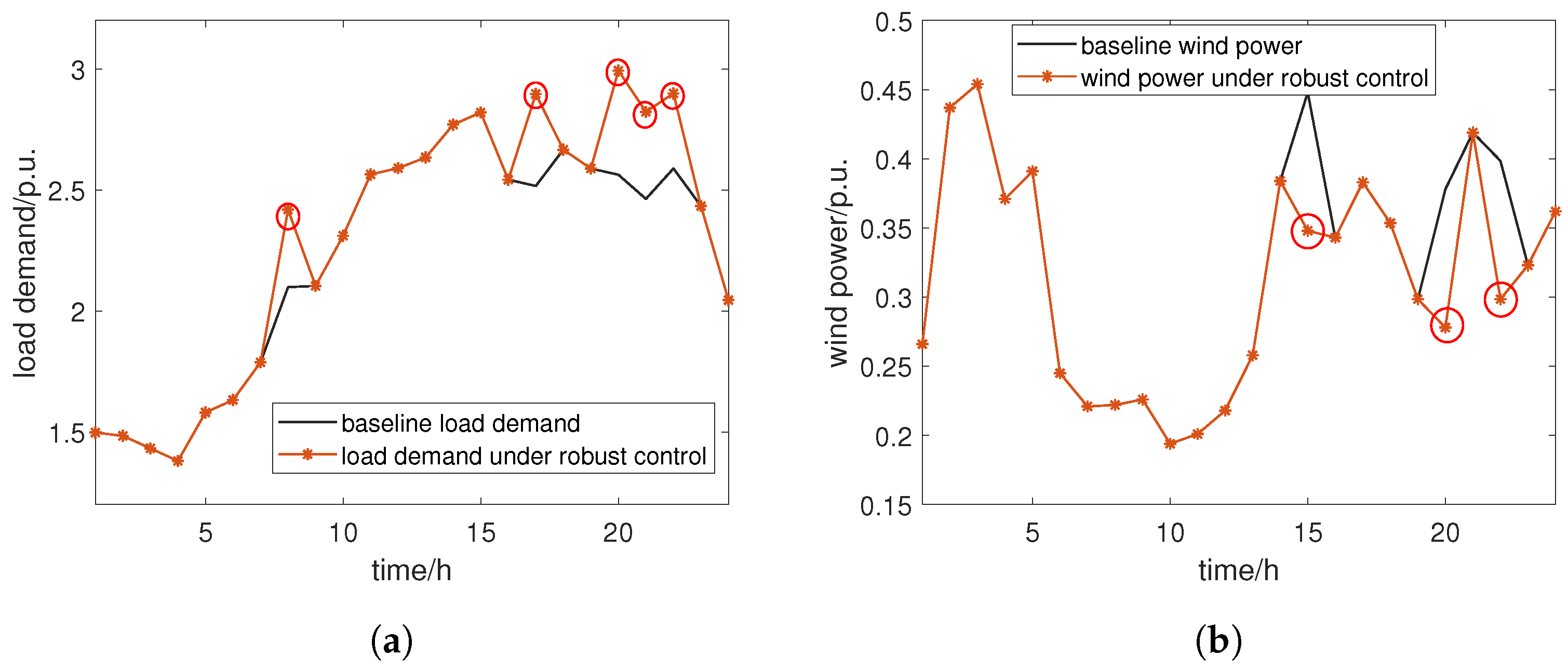
• Under the two-stage RO framework, the middle layer load and wind power uncertainties generate the worst scenario (maximum load minus minimal wind) to maximize the ramp control cost. Meanwhile the outer and inner layer ramp control sources minimize the ramp control cost and guarantee the security of operational constraints under the worst scenarios.
• Compared with the deterministic ramp control, robust ramp control uses more sources to handle the worst scenario, thus causing extra ramp control costs. Compared with the robust ramp control without the participation of HSS, the robust ramp control with HSS can significantly reduce the ramp control cost by acquiring profits in the hydrogen market.

The proposed robust strategy mainly considers exogenous parametric uncertainties. In the future, we will consider endogenous uncertainties such as decision-dependent uncertainties.

References

1. Cui, M.; Zhang, J.; Florita, A.R.; Hodge, B.M.; Ke, D.; Sun, Y. An optimized swinging door algorithm for identifying wind ramping events. IEEE Trans. Sustain. Energy 2015, 7, 150–162. [Google Scholar] [CrossRef]
2. Cui, M.; Krishnan, V.; Hodge, B.M.; Zhang, J. A copula-based conditional probabilistic forecast model for wind power ramps. IEEE Trans. Smart Grid 2018, 10, 3870–3882. [Google Scholar] [CrossRef]
3. Li, J.; Zhou, J.; Chen, B. Review of wind power scenario generation methods for optimal operation of renewable energy systems. Appl. Energy 2020, 280, 115992. [Google Scholar] [CrossRef]
4. Gao, Y.; Ma, S.; Wang, T. The impact of climate change on wind power abundance and variability in China. Energy 2019, 189, 116215. [Google Scholar] [CrossRef]
5. Boutsika, T.; Santoso, S. Quantifying short-term wind power variability using the conditional range metric. IEEE Trans. Sustain. Energy 2012, 3, 369–378. [Google Scholar] [CrossRef]
6. Niu, Y.; Santoso, S. Conditional range metric for determining wind power variability of scarce or noisy data. IEEE Trans. Sustain. Energy 2015, 6, 454–463. [Google Scholar] [CrossRef]
7. Watson, S. Quantifying the variability of wind energy. In Advances in Energy Systems: The Large-Scale Renewable Energy Integration Challenge; John Wiley & Sons, Inc.: Hoboken, NJ, USA, 2019; pp. 355–368. [Google Scholar]
8. Ren, G.; Wan, J.; Liu, J.; Yu, D. Assessing temporal variability of wind resources in China and the spatial correlation of wind power in the selected regions. J. Renew. Sustain. Energy 2020, 12, 013302. [Google Scholar] [CrossRef]
9. Garrido-Perez, J.M.; Ordóñez, C.; Barriopedro, D.; García-Herrera, R.; Paredes, D. Impact of weather regimes on wind power variability in western Europe. Appl. Energy 2020, 264, 114731. [Google Scholar] [CrossRef]
10. Barasa, M.; Aganda, A. Wind power variability of selected sites in Kenya and the impact to system operating reserve. Renew. Energy 2016, 85, 464–471. [Google Scholar] [CrossRef]
11. Feng, J.; Shen, W.Z. Wind farm power production in the changing wind: Robustness quantification and layout optimization. Energy Convers. Manag. 2017, 148, 905–914. [Google Scholar] [CrossRef]
12. Ma, X.Y.; Sun, Y.Z.; Fang, H.L. Scenario generation of wind power based on statistical uncertainty and variability. IEEE Trans. Sustain. Energy 2013, 4, 894–904. [Google Scholar] [CrossRef]
13. Wang, Z.; Shen, C.; Liu, F. A conditional model of wind power forecast errors and its application in scenario generation. Appl. Energy 2018, 212, 771–785. [Google Scholar] [CrossRef]
14. Chen, Y.; Wang, Y.; Kirschen, D.; Zhang, B. Model-free renewable scenario generation using generative adversarial networks. IEEE Trans. Power Syst. 2018, 33, 3265–3275. [Google Scholar] [CrossRef]
15. Cui, M.; Feng, C.; Wang, Z.; Zhang, J. Statistical representation of wind power ramps using a generalized Gaussian mixture model. IEEE Trans. Sustain. Energy 2017, 9, 261–272. [Google Scholar] [CrossRef]
16. Cui, M.; Zhang, J.; Wang, Q.; Krishnan, V.; Hodge, B.M. A data-driven methodology for probabilistic wind power ramp forecasting. IEEE Trans. Smart Grid 2017, 10, 1326–1338. [Google Scholar] [CrossRef]
17. Gupta, S.; Kumar, N.; Srivastava, L.; Malik, H.; Anvari-Moghaddam, A.; García Márquez, F.P. A robust optimization approach for optimal power flow solutions using Rao algorithms. Energies 2021, 14, 5449. [Google Scholar] [CrossRef]
18. Dong, J.; Yang, P.; Nie, S. Day-ahead scheduling model of the distributed small hydro-wind-energy storage power system based on two-stage stochastic robust optimization. Sustainability 2019, 11, 2829. [Google Scholar] [CrossRef]
19. Núñez-Mata, O.; Palma-Behnke, R.; Valencia, F.; Mendoza-Araya, P.; Jiménez-Estévez, G. Adaptive protection system for microgrids based on a robust optimization strategy. Energies 2018, 11, 308. [Google Scholar] [CrossRef]
20. Bertsimas, D.; Brown, D.B.; Caramanis, C. Theory and applications of robust optimization. SIAM Rev. 2011, 53, 464–501. [Google Scholar] [CrossRef]
21. Lorca, A.; Sun, X.A. Adaptive robust optimization with dynamic uncertainty sets for multi-period economic dispatch under significant wind. IEEE Trans. Power Syst. 2014, 30, 1702–1713. [Google Scholar] [CrossRef]
22. Xiong, P.; Jirutitijaroen, P.; Singh, C. A distributionally robust optimization model for unit commitment considering uncertain wind power generation. IEEE Trans. Power Syst. 2016, 32, 39–49. [Google Scholar] [CrossRef]
23. Xu, X.; Hu, W.; Cao, D.; Huang, Q.; Liu, Z.; Liu, W.; Chen, Z.; Blaabjerg, F. Scheduling of wind-battery hybrid system in the electricity market using distributionally robust optimization. Renew. Energy 2020, 156, 47–56. [Google Scholar] [CrossRef]
24. Qiu, H.; Long, H.; Gu, W.; Pan, G. Recourse-cost constrained robust optimization for microgrid dispatch with correlated uncertainties. IEEE Trans. Ind. Electron. 2020, 68, 2266–2278. [Google Scholar] [CrossRef]
25. Meng, Y.; Fan, S.; Shen, Y.; Xiao, J.; He, G.; Li, Z. Transmission and distribution network-constrained large-scale demand response based on locational customer directrix load for accommodating renewable energy. Appl. Energy 2023, 350, 121681. [Google Scholar] [CrossRef]
26. Pazouki, S.; Haghifam, M.R. Optimal planning and scheduling of energy hub in presence of wind, storage and demand response under uncertainty. Int. J. Electr. Power Energy Syst. 2016, 80, 219–239. [Google Scholar] [CrossRef]
27. Zhang, D.; Dai, Y.; Zhang, X.; Zhang, J.; Wang, Z.; Xue, L. Review and prospect of research on wind power ramp events. Power Syst. Technol. 2018, 42, 1783–1792. [Google Scholar]
28. Kamath, C. Associating weather conditions with ramp events in wind power generation. In Proceedings of the 2011 IEEE/PES Power Systems Conference and Exposition, Phoenix, AZ, USA, 20–23 March 2011; pp. 1–8. [Google Scholar]
29. Maharjan, L.; Yamagishi, T.; Akagi, H. Active-power control of individual converter cells for a battery energy storage system based on a multilevel cascade PWM converter. IEEE Trans. Power Electron. 2010, 27, 1099–1107. [Google Scholar] [CrossRef]
30. Şahin, M.E.; Blaabjerg, F. A hybrid PV-battery/supercapacitor system and a basic active power control proposal in MATLAB/simulink. Electronics 2020, 9, 129. [Google Scholar] [CrossRef]
31. Hossain Lipu, M.S.; Miah, M.S.; Ansari, S.; Meraj, S.T.; Hasan, K.; Elavarasan, R.M.; Mamun, A.A.; Zainuri, M.A.A.; Hussain, A. Power electronics converter technology integrated energy storage management in electric vehicles: Emerging trends, analytical assessment and future research opportunities. Electronics 2022, 11, 562. [Google Scholar] [CrossRef]
32. Shan, Y.; Hu, J.; Chan, K.W.; Fu, Q.; Guerrero, J.M. Model predictive control of bidirectional DC–DC converters and AC/DC interlinking converters—A new control method for PV-wind-battery microgrids. IEEE Trans. Sustain. Energy 2018, 10, 1823–1833. [Google Scholar] [CrossRef]
33. PJM Interconnection. Data Miner API Guide. 2023. Available online: https://www.pjm.com/-/media/etools/dataminer-2/data-miner-2-api-guide.ashx (accessed on 1 September 2023).
Figure 1. Power change profiles of thermal units and offshore wind farm.
Electronics 13 00211 g001
Figure 2. Schematic diagram of onshore gird connected with offshore wind farm.
Electronics 13 00211 g002
Figure 3. Schematic diagram of two-stage RO-based ramp control.
Electronics 13 00211 g003
Figure 5. Iteration process based on CC & G algorithm.
Electronics 13 00211 g005
Figure 6. Wind and load demand power profiles with and without robust ramp control. (a) load demand power profiles; (b) wind power profiles.
Electronics 13 00211 g006
Figure 7. Dispatched power of ramp control sources under robust ramp control.
Electronics 13 00211 g007
Figure 8. Wind power profiles under robust ramp control.
Electronics 13 00211 g008
Figure 9. Dispatched power of ramp control sources under deterministic ramp control.
Electronics 13 00211 g009
Figure 10. Wind power profiles under deterministic ramp control.
Electronics 13 00211 g010