
Determination of Anchor Drop Sequence during Vessel Anchoring Operations Based on Expert Knowledge Base and Hydrometeorological Conditions


Abstract
:1. Introduction
2. The Mathematical Models and Research Methodology
2.1. The Technical Specifications of the Vessel
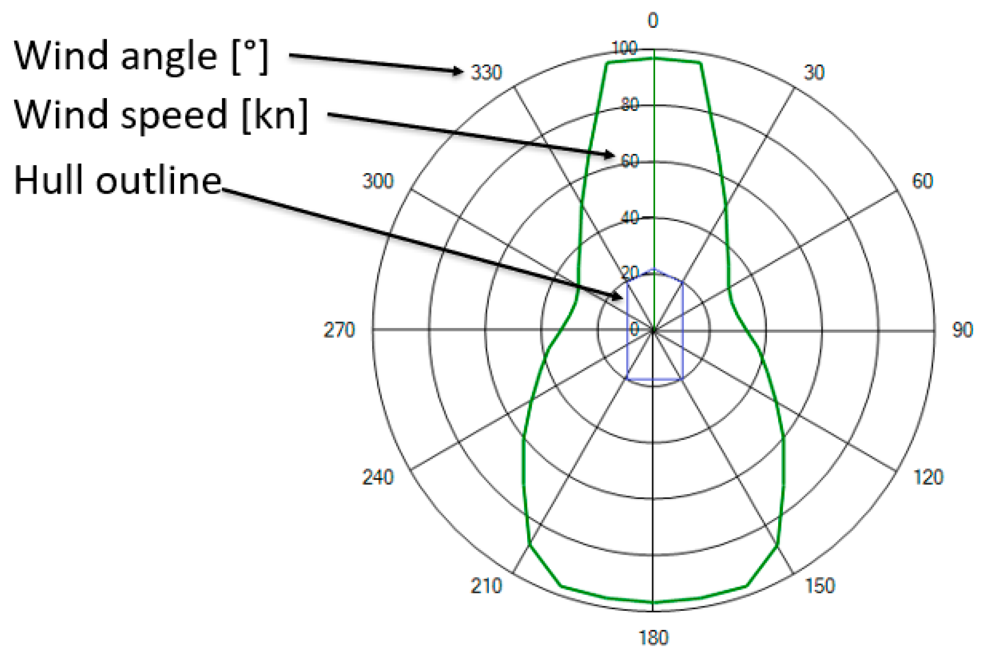
2.2. Capability Plots
- The shape located at the center of the chart represents the silhouette of the vessel;
- The numbers located on the outer periphery represent the angle of attack of environmental forces on the ship’s hull;
- The green line delineates the maximum wind speed value (in knots) that can exert an effect on the ship’s hull at a given angle while keeping the target position.
- Wind force and torque;
- Sea current force and torque;
- Sea waves force and torque.
2.2.1. Wind Force and Torque
2.2.2. Sea Current Force and Torque
2.2.3. Sea Waves Force and Torque
2.2.4. The Mathematical Model of Anchor Winch Forces
- LB—left bow anchor winch;
- RB—right bow anchor winch;
- LS—left stern anchor winch;
- RS—right stern anchor winch.
- Based on the constraints, determine initial values, and then substitute them into the system of equations.
- Check if the obtained values of the tension of each anchor winch are able to balance the given environmental forces. If not, determine a new set of values, substitute them into the equations, and recheck the solution. Repeat until a solution is found.
- Set the wind angle to 0°.
- Set the wind speed to 25 m/s and the current speed to 0.75 m/s (according to DNV guidelines).
- Calculate the environmental force value for the specified wind speed.
- Find the thrust allocation on the thrusters (or the tension in the anchor ropes) capable of resist the environmental forces.
- If a suitable force distribution capable of counteracting environmental forces is found, increase the wind speed and repeat steps 3–5. If not, decrease the wind speed and repeat steps 3–5.
- Repeat step 5 until the maximum wind speed at which the vessel can keep its position at a given wind angle is obtained. Add the point with the maximum wind value and current angle to the polar plot.
- Once the maximum wind speed for a given angle has been determined, increase the wind angle by 10°. Repeat steps 2–6.
3. Anchorage Planning Using Cognitive Knowledge Base
3.1. Cognitive Knowledge Base
- Rules related to an optimal anchor deployment field, such as:
(show anchor deployment field for anchor LB) AND
(set the maximum anchor deployment distance to 1000 m−depth)
(the initial angle between the anchor winch LB and anchor LB can be 315° ± 25°)
- Rules related to the selection of the ship’s course, for example:
(set the proposed course of the ship to 90° or 270°)
- Rules related to the selection of the anchor deployment location, such as:
(set the distance of anchor LB and RB from the ship at 35 m + a constant value) AND
(set the angle between anchor winch LB and anchor LB to 330°) AND
(set the angle between anchor winch RB and anchor RB to 30°)
(show anchor deployment field for anchor LB) AND
(set the maximum anchor deployment distance to 1000 m−depth)
| Algorithm 1: CheckDepthValue | |
| BEGIN | |
| 1: | if DepthText.text == “” or DepthText.text == null then set DepthText.text as 0 |
| 2: | if Anchor_LB == used then calculate new anchoring area and set the maximum anchor deployment distance to 1000 − float.Parse(DepthText.text) |
| 3: | if Anchor_RB == used then calculate new anchoring area and set the maximum anchor deployment distance to 1000 − float.Parse(DepthText.text) |
| 4: | if Anchor_LS == used then calculate new anchoring area and set the maximum anchor deployment distance to 1000 − float.Parse(DepthText.text) |
| 5: | if Anchor_RS == used then calculate new anchoring area and set the maximum anchor deployment distance to 1000 − float.Parse(DepthText.text) |
| END | |
- CheckDepthValue()
(adjust the rudder to achieve the desired course)
IF (ship speed != target speed) THEN
(increase the main propeller RPMs to achieve the desired speed)
(stop engines and keep position)
(anchor has not touched seabed. Loosen the anchor rope)
(anchor has not touched seabed. Loosen the anchor rope)
<(adjust the rudder to achieve the course for next anchor) AND
(increase the main propeller RPMs to achieve the desired speed)
(return to the anchor drop point) AND
(pull in the anchor) AND
(return to stage 4)
(anchor RB == dropped) AND
(anchor LS == dropped) AND
(anchor RS == dropped) THEN
(turn off main engine) AND
<pull in the anchor ropes until the ship is at the desired point>
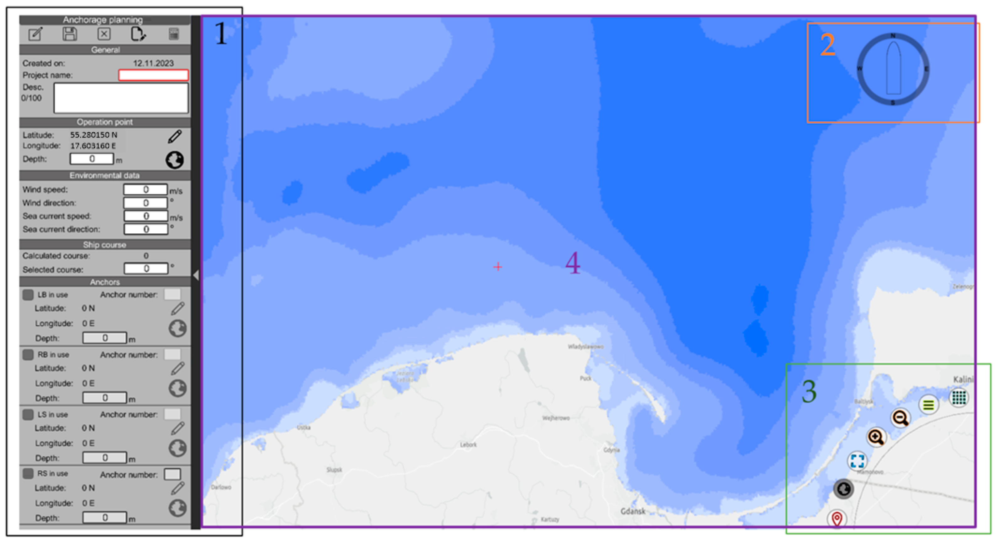
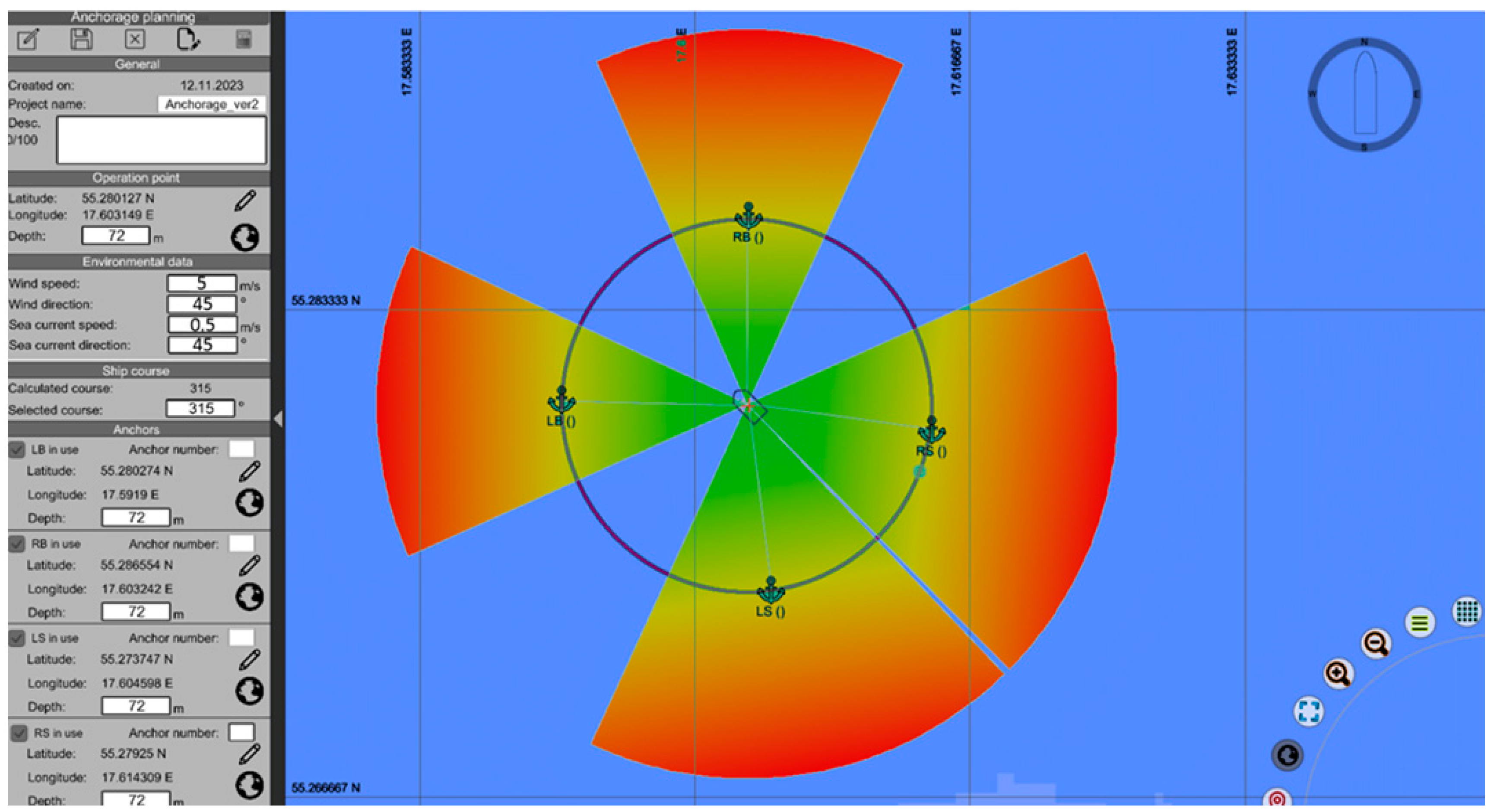
3.2. Anchorage Planning in Unity3D
- Panel for setting anchorage parameters,
- Indicator of the current course of the ship,
- Navigation tools on the map, such as zoom in/out, handling the geographic grid, and switching to a mode allowing save picture of the planned anchorage,
- Geographic grid and bathymetric map.
- “Phase”—the segment along which the ship is moving;
- “S”—the distance between the specified anchors;
- “V”—the average speed of the ship on a given phase;
- “t”—the time it takes for the ship to traverse a given phase;
- “Wind angle”—the angle of the wind force acting on the ship’s hull;
- “Env. force vector”—The vector of environmental forces acting on the ship;
- “Sum of thrust”—based on information about the interaction of environmental forces and the obtained velocity on a given phase, the algorithm determines the predicted sum of thrusters thrust;
- “Fuel consumption”—based on the thrust force values of each thruster, transit time, and technical data, the algorithm determines the average fuel consumption for a given phase;
- “Energy consumption”—based on the fuel consumption, the algorithm calculates the energy consumed. It is assumed that 1[l] ≈ 9.7 [kWh]. The efficiency of the propulsion system—41 [%].
4. Results
4.1. The Comparison of the Planned Anchor Drop Order for Two Navigation Situations in Unity3D
4.2. The Comparison of the Planned Anchor Dropping Sequence in the Anchorage Planning Tool and on the Actual Ship
- Left Side: On the left side, all parameters related to the vessel’s movement and position are displayed. This section also includes anchor-related data, such as the distance of the anchor from the ship and the length of the anchor line.
- Right Side: On the right side, there are symbols representing the ship and anchors. In the presented scenario in Figure 16, the anchors are shown to be out of range.
5. Conclusions
Author Contributions
Funding
Data Availability Statement
Conflicts of Interest
References
- Chin, C.S.; Lio, C.S. Sliding-Mode Control of STENA DRILLMAX Drillship with Environmental Disturbances for Dynamic Positioning. In Proceedings of the 11th International Conference on Modelling, Identification and Control (ICMIC2019); Wang, R., Chen, Z., Zhang, W., Zhu, Q., Eds.; Springer: Singapore, 2020; pp. 99–111. ISBN 978-981-15-0473-0. [Google Scholar]
- Machado, L.d.V.; Fernandes, A.C. Moonpool dimensions and position optimization with Genetic Algorithm of a drillship in random seas. Ocean. Eng. 2022, 247, 110561. [Google Scholar] [CrossRef]
- Bruschi, R.; Vitali, L.; Marchionni, L.; Parrella, A.; Mancini, A. Pipe technology and installation equipment for frontier deep water projects. Ocean. Eng. 2015, 108, 369–392. [Google Scholar] [CrossRef]
- International Conference on Ocean. ASME 2009 28th International Conference on Ocean, Offshore and Arctic Engineering. May 31–June 5, 2009, Honolulu, Hawaii, USA. Volume 3, Pipeline and Riser Technology; ASME: New York, NY, USA, 2009; ISBN 978-0-7918-4343-7. [Google Scholar]
- Yu, W.; Duan, C.; Kuang, C.; Zhang, H.; Wu, P.; Dai, W. Offshore towed-streamer positioning based on variance component estimation. Ocean. Eng. 2023, 278, 114355. [Google Scholar] [CrossRef]
- Wartsila. Offshore Support Vessels (OSVs). Available online: https://www.wartsila.com/encyclopedia/term/offshore-support-vessels-(osvs) (accessed on 4 November 2023).
- Chellapurath, M.; Walker, K.L.; Donato, E.; Picardi, G.; Stefanni, S.; Laschi, C.; Giorgio-Serchi, F.; Calisti, M. Analysis of Station Keeping Performance of an Underwater Legged Robot. IEEE/ASME Trans. Mechatron. 2022, 27, 3730–3741. [Google Scholar] [CrossRef]
- Peng, Z.; Wang, J.; Wang, D.; Han, Q.-L. An Overview of Recent Advances in Coordinated Control of Multiple Autonomous Surface Vehicles. IEEE Trans. Ind. Inf. 2021, 17, 732–745. [Google Scholar] [CrossRef]
- Wang, Y.; Wang, H.; Li, M.; Wang, D.; Fu, M. Adaptive fuzzy controller design for dynamic positioning ship integrating prescribed performance. Ocean. Eng. 2021, 219, 107956. [Google Scholar] [CrossRef]
- Haseltalab, A.; Negenborn, R.R. Model predictive maneuvering control and energy management for all-electric autonomous ships. Appl. Energy 2019, 251, 113308. [Google Scholar] [CrossRef]
- Walker, K.L.; Stokes, A.A.; Kiprakis, A.; Giorgio-Serchi, F. Impact of Thruster Dynamics on the Feasibility of ROV Station Keeping in Waves. In Proceedings of the Global Oceans 2020: Singapore—U.S. Gulf Coast, Biloxi, MS, USA, 5–30 October 2020; pp. 1–7, ISBN 978-1-7281-5446-6. [Google Scholar]
- Lisowski, J. Optimality of Safe Game and Non-Game Control of Marine Objects. Electronics 2023, 12, 3637. [Google Scholar] [CrossRef]
- Koznowski, W.; Kula, K.; Lazarowska, A.; Lisowski, J.; Miller, A.; Rak, A.; Rybczak, M.; Mohamed-Seghir, M.; Tomera, M. Research on Synthesis of Multi-Layer Intelligent System for Optimal and Safe Control of Marine Autonomous Object. Electronics 2023, 12, 3299. [Google Scholar] [CrossRef]
- Mohamed-Seghir, M.; Kula, K.; Kouzou, A. Artificial Intelligence-Based Methods for Decision Support to Avoid Collisions at Sea. Electronics 2021, 10, 2360. [Google Scholar] [CrossRef]
- Kaizer, A.; Winiarska, M.; Formela, K.; Neumann, T. Inland Navigation as an Opportunity to Increase the Cargo Capacity of the Tri-City Seaports. Water 2022, 14, 2482. [Google Scholar] [CrossRef]
- Guze, S.; Smolarek, L.; Weintrit, A. The area-dynamic approach to the assessment of the risks of ship collision in the restricted water. Sci. J. Marit. Univ. Szczec. 2016, 117, 88–93. [Google Scholar] [CrossRef]
- Weintrit, A. Initial Description of Pilotage and Tug Services in the Context of e-Navigation. JMSE 2020, 8, 116. [Google Scholar] [CrossRef]
- Weintrit, A. Clarification, Systematization and General Classification of Electronic Chart Systems and Electronic Navigational Charts Used in Marine Navigation. Part 2—Electronic Navigational Charts. TransNav 2018, 12, 769–780. [Google Scholar] [CrossRef]
- Rak, A.; Miller, A. Modelling of Lake Waves to Simulate Environmental Disturbance to a Scale Ship Model. Pol. Marit. Res. 2023, 30, 12–21. [Google Scholar] [CrossRef]
- Rybczak, M.; Gierusz, W. Maritime Autonomous Surface Ships in Use with LMI and Overriding Trajectory Controller. Appl. Sci. 2022, 12, 9927. [Google Scholar] [CrossRef]
- Soliwoda, J.; Kaizer, A.; Neumann, T. Possibility of Capsizing of a Dredger during Towing. Water 2021, 13, 3027. [Google Scholar] [CrossRef]
- Madadi, B.; Aksakalli, V. A stochastic approximation approach to spatio-temporal anchorage planning with multiple objectives. Expert Syst. Appl. 2020, 146, 113170. [Google Scholar] [CrossRef]
- Oz, D.; Aksakalli, V.; Alkaya, A.F.; Aydogdu, V. An anchorage planning strategy with safety and utilization considerations. Comput. Oper. Res. 2015, 62, 12–22. [Google Scholar] [CrossRef]
- Jajac, N.; Kilić, J.; Rogulj, K. An Integral Approach to Sustainable Decision-Making within Maritime Spatial Planning—A DSC for the Planning of Anchorages on the Island of Šolta, Croatia. Sustainability 2019, 11, 104. [Google Scholar] [CrossRef]
- Abramowicz-Gerigk, T.; Burciu, Z.; Jaworski, T.; Nowicki, J. The Large-Scale Physical Model Tests of the Passing Ship Effect on a Ship Moored at the Solid-Type Berth. Sensors 2022, 22, 868. [Google Scholar] [CrossRef] [PubMed]
- Przybylowski, A.; Suchanek, M.; Miszewski, P. COVID-19 Pandemic Impact on a Global Liner Shipping Company Employee Work Digitalization. TransNav 2022, 16, 759–765. [Google Scholar] [CrossRef]
- Dang, X.-K.; Do, V.-D.; Nguyen, X.-P. Robust Adaptive Fuzzy Control Using Genetic Algorithm for Dynamic Positioning System. IEEE Access 2020, 8, 222077–222092. [Google Scholar] [CrossRef]
- Fossen, T.I. Handbook of Marine Craft Hydrodynamics and Motion Control; Wiley: Hoboken, NJ, USA, 2011. [Google Scholar]
- Walker, K.L.; Gabl, R.; Aracri, S.; Cao, Y.; Stokes, A.A.; Kiprakis, A.; Giorgio-Serchi, F. Experimental Validation of Wave Induced Disturbances for Predictive Station Keeping of a Remotely Operated Vehicle. IEEE Robot. Autom. Lett. 2021, 6, 5421–5428. [Google Scholar] [CrossRef]
- Robert Stewart. Ocean-Wave Spectra. Available online: https://wikiwaves.org/Ocean-Wave_Spectra (accessed on 5 November 2023).
- DNV. Main Website. Available online: https://www.dnv.com/index.html (accessed on 5 November 2023).
- DNV Rules and Standards. Assessment of Station Keeping Capability of Dynamic Positioning Vessels. Available online: https://standards.dnv.com/explorer/document/7E231C260D4846DF8DF3CBA12A2229D4/5 (accessed on 12 December 2023).


| Parameter | Value |
|---|---|
| Length overall (Loa) [m]: | 72.7 |
| Length between perpendiculars (Lpp) [m]: | 64 |
| Breadth [m]: | 11.6 |
| Draught [m]: | 3.4 |
| Displacement [T]: | 1886 |
| Distance between foremost and aft most point of the hull below the surface at design draft even keel [m]: | 67.1 |
| Water plane area [m2]: | 639 |
| Projected longitudinal area above water [m2]: | 437 |
| Surge position of geometric center of the projected longitudinal area above water with respect to Lpp/2 [m]: | 0.1 |
| Projected longitudinal area below water [m2]: | 223 |
| Surge position of geometric center of the projected longitudinal area below water with respect to Lpp/2 [m]: | −2.9 |
| Surge position of water line center with respect to Lpp/2 [m]: | −1.5 |
| Projected transverse area above water [m2]: | 140 |
| Projected transverse area below water [m2]: | 36 |
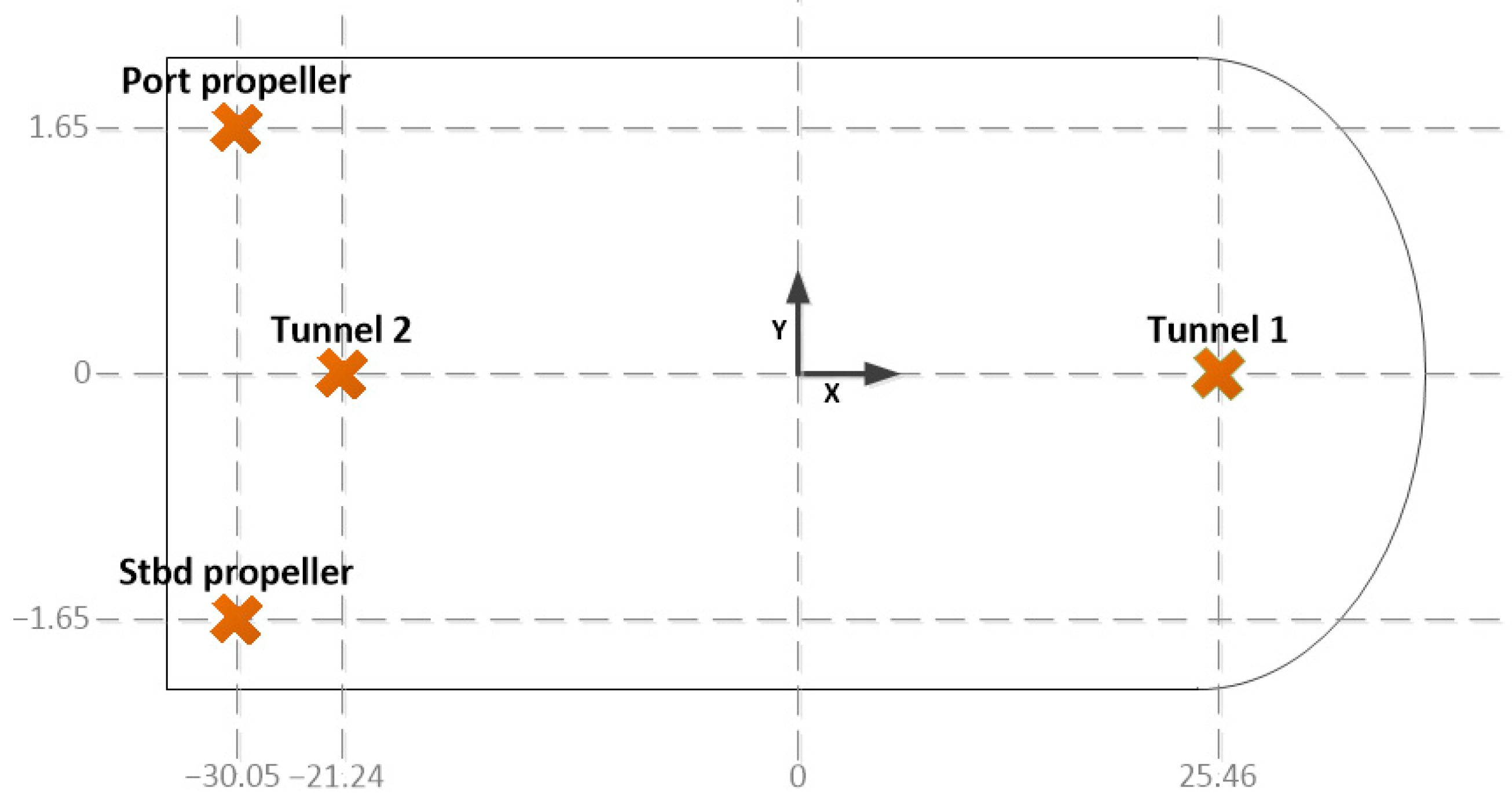
| Thruster | Thrust Max [kN] | Thrust Min [kN] | Power [kW] |
|---|---|---|---|
| Tunnel 1 | 94 | −94 | 447 |
| Tunnel 2 | 94 | −94 | 447 |
| Port propeller | 179 | −179 | 2000 |
| Stbd propeller | 179 | −179 | 2000 |
| Winch | Max Pull [kN] (500 m Rope) | Max Pull [kN] (750 m Rope) | Max Pull [kN] (1000 m Rope) |
|---|---|---|---|
| LB | 102.53 | 116.47 | 124.85 |
| RB | 102.53 | 116.47 | 124.85 |
| LS | 102.53 | 116.47 | 124.85 |
| RS | 102.53 | 116.47 | 124.85 |
| Parameter | Value |
|---|---|
| Initial angle between anchor winch LB and anchor LB | 315° ± 25° |
| Initial angle between anchor winch RB and anchor RB | 45° ± 25° |
| Initial angle between anchor winch LS and anchor LS | 225°± 35° |
| Initial angle between anchor winch RS and anchor RS | 135°± 35° |
| Maximum length of the deployed anchor rope [m] | 1000 |
| Minimum length of the deployed anchor rope [m] | 100 |
| Fuel consumption at 100% main engine load [l/h] | 246 |
| Fuel consumption at 100% tunel thruster load [l/h] | 37 |
| Phase | S [NM] | V [knots] | t [h] | Wind Angle [°] | Env. Force Vector (x-Axis; y-Axis) | Sum of Thrust [kN] | Fuel Consumption [l] | Energy Consumption [kWh] |
|---|---|---|---|---|---|---|---|---|
| RB -> LB | 0.6 | 0.4 | 1.5 | 90 | (0.5 kN; 46 kN) | 137 | 71.61 | 318.66 |
| LB -> RS | 0.84 | 0.4 | 2.1 | 135 | (6 kN; 34 kN) | 152 | 156.89 | 698.16 |
| RS -> LS | 0.6 | 0.4 | 1.5 | 90 | (0.5 kN; 46 kN) | 137 | 71.64 | 318.79 |
| SUM | 1335.74 |
| Case | Phase | S [NM] | V [knots] | t [h] | Wind Angle [°] | Env. Force Vector (x-axis; y-axis) | Sum of Thrust [kN] | Fuel Consumption [l] | Energy Consumption [kWh] |
|---|---|---|---|---|---|---|---|---|---|
| 1 | RB -> LB | 0.6 | 0.4 | 1.5 | 0 | (7.5 kN; 0 kN) (5.2 kN; 34 kN) (7.5 kN; 0 kN) | 189 | 110.41 | 446.22 |
| LB -> RS | 0.84 | 0.4 | 2.1 | 45 | 138 | 170.88 | 690.62 | ||
| RS -> LS | 0.6 | 0.4 | 1.5 | 0 | 189 | 110.43 | 446.31 | ||
| SUM | 1538.13 | ||||||||
| 2 | RB -> LB | 0.6 | 0.4 | 1.5 | 0 | (7.5 kN; 0 kN) | 189 | 110.41 | 446.24 |
| LB -> LS | 0.6 | 0.4 | 1.5 | 0 | (7.5 kN; 0 kN) | 60 | 118.08 | 477.23 | |
| LS -> RS | 0.6 | 0.4 | 1.5 | 0 | (7.5 kN; 0 kN) | 189 | 110.39 | 446.15 | |
| SUM | 1369.62 | ||||||||
| 3 | LB -> RB | 0.6 | 0.4 | 1.5 | 0 | (7.5 kN; 0 kN) | 189 | 110.43 | 446.32 |
| RB -> RS | 0.6 | 0.4 | 1.5 | 0 | (7.5 kN; 0 kN) | 60 | 118.11 | 477.36 | |
| RS -> LS | 0.6 | 0.4 | 1.5 | 0 | (7.5 kN; 0 kN) | 189 | 110.42 | 446.26 | |
| SUM | 1369.94 | ||||||||
| 4 | LB -> RB | 0.6 | 0.4 | 1.5 | 0 | (7.5 kN; 0 kN) | 189 | 110.39 | 446.14 |
| RB -> LS | 0.84 | 0.4 | 2.1 | 315 | (5.2 kN; 34 kN) | 138 | 170.91 | 690.76 | |
| LS -> RS | 0.6 | 0.4 | 1.5 | 0 | (7.5 kN; 0 kN) | 189 | 110.41 | 446.24 | |
| SUM | 1583.14 |
| Case | Phase | S [NM] | V [knots] | t [h] | Wind Angle [°] | Env. Force Vector (x-Axis; y-Axis) | Sum of Thrust [kN] | Fuel Consumption [l] | Energy Consumption [kWh] |
|---|---|---|---|---|---|---|---|---|---|
| 1 | RB -> LB | 0.09 | 0.29 | 0.31 | 66 | (3 kN; 41 kN) (5 kN; 33 kN) (0.5 kN; 48 kN) | 74 | 6.75 | 27.28 |
| LB -> RS | 0.18 | 0.21 | 0.9 | 137 | 82 | 36.26 | 146.55 | ||
| RS -> LS | 0.11 | 0.29 | 0.37 | 92 | 76 | 8.67 | 35.04 | ||
| SUM | 208.87 | ||||||||
| 2 | RB -> LB | 0.14 | 0.4 | 0.35 | 92 | (0.5 kN; 48 kN) | 76 | 8.48 | 34.27 |
| LB -> RS | 0.21 | 0.4 | 0.52 | 137 | (5 kN; 33 kN) | 82 | 31.49 | 127.27 | |
| RS -> LS | 0.14 | 0.4 | 0.35 | 92 | (0.5 kN; 48 kN) | 76 | 8.53 | 34.47 | |
| SUM | 196.01 |
Disclaimer/Publisher’s Note: The statements, opinions and data contained in all publications are solely those of the individual author(s) and contributor(s) and not of MDPI and/or the editor(s). MDPI and/or the editor(s) disclaim responsibility for any injury to people or property resulting from any ideas, methods, instructions or products referred to in the content. |
© 2023 by the authors. Licensee MDPI, Basel, Switzerland. This article is an open access article distributed under the terms and conditions of the Creative Commons Attribution (CC BY) license (https://creativecommons.org/licenses/by/4.0/).
Share and Cite
Wnorowski, J.; Łebkowski, A. Determination of Anchor Drop Sequence during Vessel Anchoring Operations Based on Expert Knowledge Base and Hydrometeorological Conditions. Electronics 2024, 13, 176. https://doi.org/10.3390/electronics13010176
Wnorowski J, Łebkowski A. Determination of Anchor Drop Sequence during Vessel Anchoring Operations Based on Expert Knowledge Base and Hydrometeorological Conditions. Electronics. 2024; 13(1):176. https://doi.org/10.3390/electronics13010176
Chicago/Turabian StyleWnorowski, Jakub, and Andrzej Łebkowski. 2024. "Determination of Anchor Drop Sequence during Vessel Anchoring Operations Based on Expert Knowledge Base and Hydrometeorological Conditions" Electronics 13, no. 1: 176. https://doi.org/10.3390/electronics13010176