A Sliding Mode Controller with Signal Transmission Delay Compensation for the Parallel DC/DC Converter’s Network Control System

Abstract

The network control system (NCS) of the parallel DC/DC converter is always affected by the signal transmission delay, and the ideal output performance is lost. In this paper, a typical parallel buck converter is taken as the research object. Firstly, a sliding mode controller (SMC) in the discrete domain is designed to enhance the robustness of the system. On this basis, the effects of different delays on the stability of the converter’s NCS are analyzed, and the actual effects of long/short delays on the converter’s NCS are obtained. To further solve the problem of damage to transmitted signals of the NCS by long delay, the SM controller designed in this paper is improved by incorporating a multi-step prediction method. This enhancement enables effective prediction and compensation of the delay signals lost by the NCS, ensuring the output performance of the parallel buck converter. Finally, the superiority of the proposed method is verified by designing simulations and experiments.

1. Introduction

The parallel DC/DC converter finds extensive application across various domains, including electric vehicles, photovoltaic systems, telecommunication base stations, and other electric energy conversion fields [1,2]. Its remarkable attributes include the mitigation of physical stress on the converter during energy flow by employing voltage equalization and parallel techniques [3,4]. Consequently, these features contribute to the enhancement of the converter’s output power [5,6].

In engineering applications, network control systems (NCSs) are employed to manage parallel DC/DC converters because of their ease of deployment and operation [7,8]. Since the control signals for parallel DC/DC converters as well as the status signals from sensors and actuators are transmitted via network channels, the network transmission is often assumed to be ideal during the system design phase [9,10]. However, practical experience reveals that, owing to limitations in network bandwidth and signal processing speed, network controllers exhibit signal transmission delays, resulting in packet loss [10,11]. This phenomenon significantly impairs the stability of the control system’s output [12,13]. Furthermore, the network signal transmission delay and packet loss rate are influenced by various factors that change over time, rendering them highly uncertain [14,15]. Given the random occurrence of network transmission delays and packet losses, selecting and adjusting the signal sampling period for parallel DC/DC converters is a formidable challenge. This not only impacts the quality of the converter’s output power but also hampers the overall control performance enhancement of the NCS [16,17].

When comparing the delay in network transmission with the system sampling period, the delay can be categorized into two types: short delay and long delay. Short delay refers to cases where the signal transmission delay is less than or equal to a single sampling period, while long delay occurs when the delay exceeds the sampling period [18,19]. Addressing the impact of these different delays on NCS has emerged as a prominent research area. Initially, Pang et al. assumed that the signal transmission delay between the sensor, controller, and actuator made up a short delay. Accordingly, they developed a controller that considered the impact of this delay. However, this method’s reliance on the assumption of only short delays overlooked the possibility of encountering long delays, thereby imposing limitations on its effectiveness [20]. Yan et al. designed an event-triggered H∞ controller for NCSs with network channel delay. The network channel delay is modeled as a distributed delay with a probability density function as its kernel, and the closed-loop event-triggered control system is established as a distributed delay system. However, the method proposed in the literature is based on the continuous domain without exploiting the potential influence of discretization on the stability of the event-triggered H∞ controller. Hence, the implementation and application performance of the designed method is reduced [21]. Kim et al. proposed a new method to obtain a maximum allowable delay bound for the scheduling of NCSs. The method is planned in terms of linear matrix inequalities and can provide a much less conservative delay bound than the existing methods, and a network scheduling method is presented based on the delay obtained through the proposed method. However, the method of obtaining the transmission delay of NCSs is not clearly provided in the literature, and only the estimated delay length is used to assign network nodes to the transmission signal of the system, which reduces the reliability of the system [22]. Heemels et al. presented a general framework that incorporates communication constraints, varying transmission intervals and varying delays, and an explicit construction of a continuum of Lyapunov functions is provided based on a newly developed NCS model including all these network phenomena, then the maximally allowable transmission interval and the maximally allowable delay to guarantee stability of the NCS in the presence of communication constraints. However, the literature has not put forward an exact and effective solution for different transmission intervals and delays [23]. Bibhu et al. presented the development of a novel synchrophasor measurement-based wide-area centralized damping controller to improve the stability of a power system in the presence of time-varying delay and packet dropout in the communication network. This method depends on the measurement of the transmission delay itself, which requires high precision of the control system [24]. In this literature [25], a networked predictive control strategy is proposed for discrete networked systems to deal with the random delay. However, this method treats the network transmission delay as a fixed delay and cannot be applied to complex network delays. Based on the analysis provided, most studies predominantly focus on the continuous time domain, neglecting the discrete state of NCSs and the nuanced performance analysis concerning various types of delays affecting the system. And the problem of measuring the transmission delay of the system has become a difficult problem restricting the design of the controller, the challenge of effectively compensating random delays in control signals of NCSs requires further improvement. This paper systematically considers the practicability of continuous domain control design and discrete domain controller transformation, analyze the impact of different types of delay on the system NCS, and use the signal retention characteristics of the sensor to avoid the measurement of transmission delay.

A large amount of literature shows that the application of sliding mode control (SMC) in parallel DC/DC converters combines robustness, fast response, and enhanced current-sharing capabilities. These advantages make the SMC strategy an attractive choice for enhancing the performance and reliability of parallel DC/DC converter systems [26,27]. The literature [28] proposes a novel nonlinear control method for the input-parallel output-series modular dual active bridge DC/DC converter, which regulates the DC-bus voltage and individual module voltages together. A uniform quantization design method for the parallel text DC-DC converter’s NCS is proposed in [29] in combination with the SMC strategy to solve the problem that the performance of the system is poor. The literature [30] shows the analysis and design of a parallel-connected converter system using sliding mode control techniques. And a new general SMC is proposed for the DC-DC converter that can regulate the output voltage in the literature [31]. The literature [32] also presents a control design procedure for DC-DC power converters, which develops SMC algorithms for several types of DC-DC converters with different control objectives, and complete and incomplete information about system states.

In this paper, a discrete domain SM current-sharing controller based on linear sliding mode control (LSMC) strategy is designed for the parallel DC/DC converter’s NCS, with the buck type being used as an example. The study focuses on analyzing the impact of uncertain and random transmission delays on performing the parallel buck converter’s NCS, particularly in the presence of system disturbances. To address this, a multi-step prediction method is employed for compensating the delay signal in the NCS. The article makes the following specific contributions:

• Considering a parallel buck converter’s NCS with a random time delay, a master-slave current-sharing controller is designed based on the LSMC in the continuous domain. Then the zero-order holder (ZOH) is used to realize the discretization of the designed system, and the stability conditions of the discrete system are further determined through the Lyapunov equation;
• Based on the length characteristics of different transmission delays, the effects of uncertainty and randomness on performing parallel buck converter’s NCS with system disturbance are analyzed, which lays a foundation for the design of delay compensation strategy;
• In order to solve the problem of the influence of random delay on the system stability, the LSM controller is improved based on the multi-step prediction method, and the system parameter conditions are provided based on analyzing the stability of the designed control system;
• Designed simulations and experiments prove the effectiveness of the proposed method.

2. Design of SMC for the Parallel DC/DC Converter

This paper takes a typical n-phase parallel buck converter system as an example of designing its NCS. The overall structure of the system is shown in Figure 1 below.

In Figure 1, E is the DC input voltage source; v_O is the output voltage of the parallel buck converter; R is the load resistance; L_i and C_i represent the filter inductance and capacitance of phase i (i = 1, 2, …, n), respectively; i_Li and i_Ci represent the current flowing through L_i and C_i, respectively; i_Ri indicates the current output of each phase to load R, and satisfying i_Ri = i_Li − i_Ci; VD_i is phase i continuous current diode; S_wi represents the phase i switching power tube, often used by N-MOSFET or IGBT, whose “on” and “off” state are controlled by the “1” and “0” pulses of the signal u_i; V_ref represents the output reference voltage of the converter; and s_i is the system state variable output by the SM controller.

In order to be closer to the real NCS, the time delay of signal transmission between the feedforward channel and the feedback channel is considered in Figure 1, and it is assumed that the delay from the sensor to the controller is τ_s, the delay from the controller to the actuator is τ_c. In fact, if the feedback control system can maintain static properties, these two delays can be lumped together as τ = τ_s + τ_c, and the τ is the total delay in the NCS [31]. For the convenience of description, the subscript “τ” is used to represent signals with transmission delays, such as i_Liτ, v_Oτ, and u_iτ. It should be noted here that the delay τ does not change the characteristics of the signal itself, such as u_iτ and u_i are all output “1” or “0” control signals.

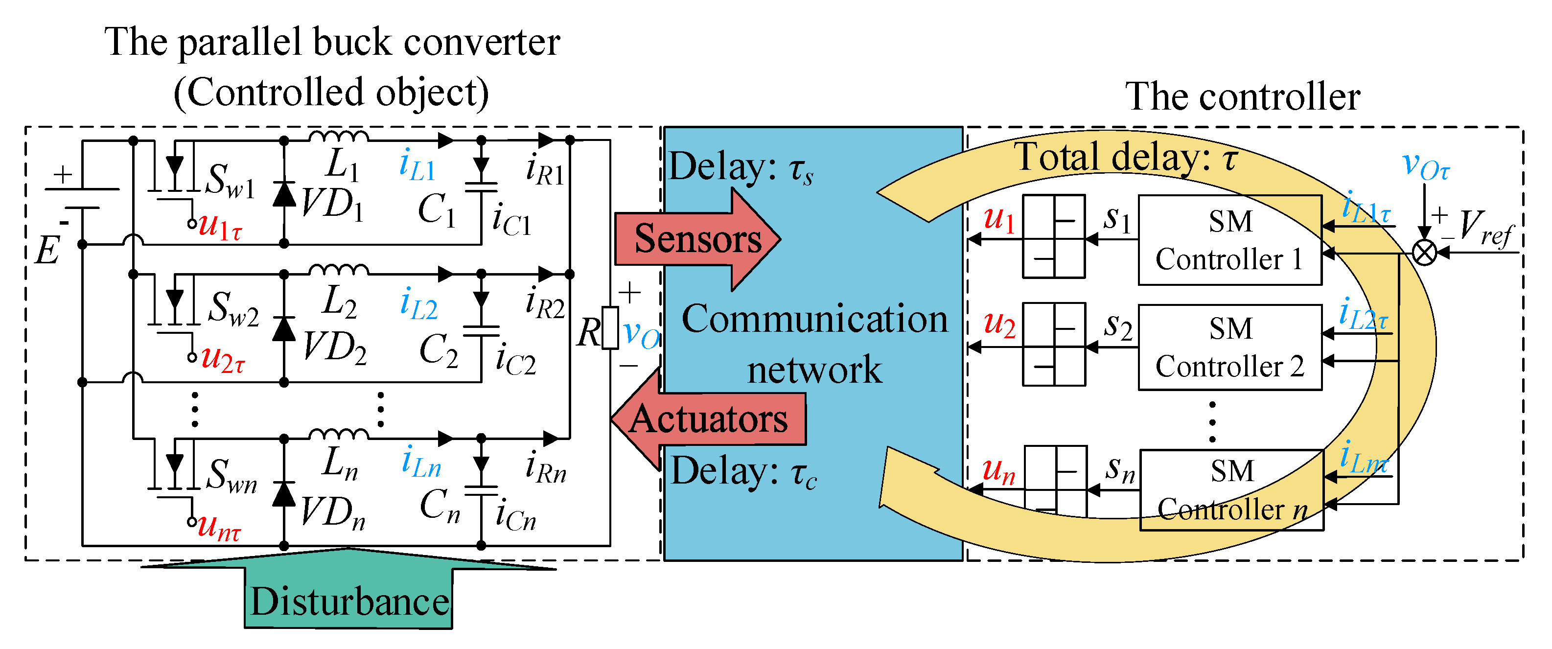
2.1. Modeling of the Parallel Buck Converter System

In order to facilitate the analysis of the energy flow process of the converter, the switching loss of the converter is ignored here, and it is assumed that the parallel buck converter works in continuous current mode (CCM), and each phase control signal u_τ is generated by the same pulse width modulation (PWM). Thus, the output current of each phase of the system can meet i_Ri = v_O/(nR). By analyzing the working process of the converter when the power tube S_wi is switched on and off, and combining Kirchhoff’s circuit law and the characteristics of L_i and C_i components, the following converter model can be obtained:

$$S_{wi} \mathrm{on} \left\{\begin{array}{l}\frac{\mathrm{d}{i}_{Li}}{\mathrm{d}t}=\frac{1}{L_i}\left(E-v_O\right)\\ \frac{\mathrm{d}{v}_O}{\mathrm{d}t}=\frac{1}{C_i}{i}_{Ci}=\frac{1}{C_i}\left(i_{Li}-i_{Ri}\right)\end{array}\right., S_{wi} \mathrm{off} \left\{\begin{array}{l}\frac{\mathrm{d}{i}_{Li}}{\mathrm{d}t}=-\frac{1}{L_i}{v}_O\\ \frac{\mathrm{d}{v}_O}{\mathrm{d}t}=\frac{1}{C_i}\left(i_{Li}-i_{Ri}\right)\end{array}\right.$$

(1)

Using the characteristic of control signal u_iτ output “0” or “1”, and substituting i_Ri = v_O/(nR) into (1), then the system model can be represented uniformly as:

$$\left[\begin{array}{c}\frac{\mathrm{d}{i}_{Li}}{\mathrm{d}t}\\ \frac{\mathrm{d}{v}_O}{\mathrm{d}t}\end{array}\right]=\left[\begin{array}{cc}0& -\frac{1}{L_i}\\ \frac{1}{C_i}& -\frac{1}{nR{C}_i}\end{array}\right]\left[\begin{array}{c}{i}_{Li}\\ v_O\end{array}\right]+\left[\begin{array}{c}\frac{E}{L_i}\\ 0\end{array}\right]u_{i\tau }$$

(2)

2.2. Design of the SM Controller

Due to the simple structure of LSM, the impulse switching control of u_iτ signal can be satisfied on the basis of ensuring the robustness of the system [29]. Therefore, this paper adopts the LSM to design the parallel DC/DC converter control system in the continuous domain. For the circuit topology is shown in Figure 1, the phase i is taken as the object, and the output voltage deviation and its derivative of the phase i are respectively defined as state variables x_1iτ and x_2iτ as:

$$\left\{\begin{array}{l}{x}_{1i\tau }=v_{O\tau }-V_{ref}\\ x_{2i\tau }={\dot{x}}_{1i\tau }={\dot{v}}_{O\tau }\end{array}\right.$$

(3)

where V_ref is the reference value of the output voltage v_Oτ of the converter; x_1iτ and x_2iτ are bounded variables and satisfy |x_1iτ| ≤ ψ_x1iτ and |x_1iτ| ≤ ψ_x2iτ, ψ_x1iτ > 0 and ψ_x2iτ > 0 are boundary constants. By further substituting (2) into (3), the state space model of the buck system can be obtained as:

$${\dot{\mathit{x}}}_{i\tau }\left(t\right)={\mathit{A}}_i{\mathit{x}}_{i\tau }\left(t\right)+{\mathit{b}}_i{u}_{i\tau }\left(t\right)+{\mathit{f}}_i+{\mathit{\zeta }}_i\left(t\right)$$

(4)

where the state vector x_iτ(t) = [x_1iτ(t), x_2iτ(t)]^T, and there is ||x_iτ(t)|| ≤ ψ_xiτ, ψ_xiτ = [ψ_x1iτ, ψ_x2iτ]^T is the boundary constant vector; ζ_i(t) is the matching disturbance of the system, which satisfying ζ_i(t) = b_iδ_i(t), where δ_i is the actual bounded disturbance of the external input, which satisfying |δ_i(t)| ≤ β_i, and β_i is the upper bound constant. The coefficient matrix A_i, b_i, and f_i can be expressed as:

$${\mathit{A}}_i=\left[\begin{array}{cc}0& 1\\ -\frac{1}{L_i{C}_i}& -\frac{1}{nR{C}_i}\end{array}\right], {\mathit{b}}_i=\left[\begin{array}{c}0\\ \frac{E}{L_i{C}_i}\end{array}\right], {\mathit{f}}_i=\left[\begin{array}{c}0\\ -\frac{V_{ref}}{L_i{C}_i}\end{array}\right]$$

(5)

The design of LSMC generally includes LSM surface and control law. And the LSM surface of the system can be designed by the state variables in (4) as:

$$s_i\left(t\right)={\lambda }_i{x}_{1i\tau }\left(t\right)+x_{2i\tau }\left(t\right)+k_i{\displaystyle {\int }_0^t{x}_{1i\tau }\left(t\right)\mathrm{d}t}$$

(6)

where s_i(t) is the sliding variable of the phase i controller; λ_i and k_i are the coefficients of the SM surface, and satisfying λ_i > 0 and k_i > 0.

Remark 1.

It should be noted that λ_i can be used to adjust the convergence rate of the s_i(t) of the system, but the chattering of the system state will also be aggravated with the increase in λ_i. Hence the integral term is introduced in (6) to help adjust the steady-state error of the system output and further enhance the robustness of SMC. And it is necessary to analyze the motion characteristics of the designed sliding surface in (6):

When the system state reaches the preset SM surface s_i(t) = 0, it can be obtained that:

$${\ddot{x}}_{1i\tau }\left(t\right)+{\lambda }_i{\dot{x}}_{1i\tau }\left(t\right)+k_i{x}_{1i\tau }\left(t\right)=0$$

(6a)

Here defining x_1iτ(0) and x_2iτ(0) = ${\dot{x}}_{1i\tau }(0)$as the initial values of x_1iτ(t) and x_2iτ(t). By introducing the Laplace transform, can we get the unique solution to (6a) as:

$$x_{1i\tau }(t)=\frac{x_{1i\tau }\left(0\right)\left(2-{\lambda }_i+\sqrt{{\lambda }_i^2-4k_i}\right)+{\dot{x}}_{1i\tau }\left(0\right)}{2\sqrt{{\lambda }_i^2-4k_i}}{e}^{\frac{-{\lambda }_i+\sqrt{{\lambda }_i^2-4k_i}}{2}t}+\frac{x_{1i\tau }\left(0\right)\left(2-{\lambda }_i-\sqrt{{\lambda }_i^2-4k_i}\right)+{\dot{x}}_{1i\tau }\left(0\right)}{-2\sqrt{{\lambda }_i^2-4k_i}}{e}^{\frac{-{\lambda }_i-\sqrt{{\lambda }_i^2-4k_i}}{2}t}$$

(6b)

It can be obviously seen from (6b) that the coefficient k_i can be used to adjust the convergence rate of the exponential terms in each term, which not only avoids the chattering problem caused by the use of larger λ_i, but also clearly provides the limit range λ_i² > 4k_i of λ_i, i.e., the selection of k_i should also be smaller to improve the output accuracy of the system.

As for the control law u_siτ(t) of the LSMC in the phase i, which is usually composed of the equivalent control law u_eqiτ(t) and the switching control law u_Niτ(t). In the process of system convergence, the system state rapidly reaches the preset SM surface s_i(t) = 0 under the action of u_eqiτ(t), and then moves along s_i(t) = 0 under the action of u_Niτ(t) to the convergence point. Combining the above state motion characteristics of the SMC system, u_eqiτ(t) can be obtained by finding the zero crossing of the first derivative of s_i(t) in (6). Therefore, the first derivative of s_i(t) and the system state variable in (3) can be substituted into it as:

$${\dot{s}}_i\left(t\right)=-\frac{1}{L_i{C}_i}{x}_{1i\tau }\left(t\right)+\left({\lambda }_i-\frac{1}{nR{C}_i}\right)x_{2i\tau }\left(t\right)+\frac{E}{L_i{C}_i}{u}_{si\tau }\left(t\right)-\frac{V_{ref}}{L_i{C}_i}+\frac{E}{L_i{C}_i}{\delta }_i\left(t\right)$$

(7)

In (7), if ${\left.{\dot{s}}_i\left(t\right)\right|}_{u_{eqi\tau }}=0$, the expression of u_eqiτ(t) can be expressed as:

$$u_{eqi\tau }\left(t\right)=\frac{1}{E}{x}_{1i\tau }\left(t\right)-\frac{L_i{C}_i}{E}\left({\lambda }_i-\frac{1}{nR{C}_i}\right)x_{2i\tau }\left(t\right)+\frac{V_{ref}}{E}-{\delta }_i\left(t\right)$$

(8)

Considering the switching characteristics of the parallel buck converter corresponding to (1), u_Niτ(t) can be further designed as:

$$u_{Ni\tau }\left(t\right)=-{\eta }_i\mathrm{sgn}\left[s_i\left(t\right)\right]$$

(9)

where η_i is the switching control gain and satisfying η_i > 0. By combining (8) and (9), the control law u_siτ(t) of LSM can be obtained as:

$$u_{si\tau }\left(t\right)=u_{eqi\tau }\left(t\right)+u_{Ni\tau }\left(t\right)=k_{\mathrm{PWM}}{u}_{i\tau }\left(t\right)$$

(10)

where k_PWM represents the required gain after the continuous control signal u_siτ(t) is converted into the switching signal u_iτ(t) by PWM. According to the literature [33], u_siτ(t) is essentially the switching duty cycle of the converter, so the LSMC designed in this paper is essential to adjust the output voltage of the system by controlling the switching duty cycle of the parallel buck converter.

2.3. Discretization and Stability Analysis of the System

In order to further expand the application of the designed SMC system in digital circuits and facilitate the analysis of the transmission delay process of the NCS, the SMC of the parallel buck converter designed in (4), (6), and (10) will be discretized. Here the ZOH is used to discretize the system, and system states in (4) can be transformed into:

$${\mathit{x}}_{i\tau }\left[\left(k+1\right)h\right]={\mathit{\Phi }}_i{\mathit{x}}_{i\tau }\left(kh\right)+{\mathit{\Gamma }}_i{u}_{si\tau }\left(kh\right)+{\mathit{\Lambda }}_i+{\mathit{\Gamma }}_i{\delta }_i\left(kh\right)$$

(11)

where x_iτ(kh) = [x_1iτ(kh), x_2iτ(kh)]^T represents the state of the discrete system, and relationship of ||x_iτ(kh)|| ≤ ψ_xiτ is held; u_siτ(kh) stands for the discrete control law; h is the signal sampling period, and satisfying 0 < h << 1; the expressions of the discrete coefficient matrix Φ_i, Γ_i and Λ_i can be expressed as:

$$\left\{\begin{array}{l}{\mathit{\Phi }}_i=e^{{\mathit{A}}_{i}h}=\mathit{I}+{\displaystyle {\int }_0^h{e}^{{\mathit{A}}_{i}t}dt{\mathit{A}}_i}=\mathit{I}+{\mathit{A}}_{i}h+{\mathit{A}}_i^2\frac{h^2}{2!}+O\left(h^3\right)\\ {\mathit{\Gamma }}_i={\displaystyle {\int }_0^h{e}^{{\mathit{A}}_{i}t}dt{\mathit{b}}_i}={\mathit{b}}_{i}h+{\mathit{A}}_i{\mathit{b}}_i\frac{h^2}{2!}+O\left(h^3\right)\\ {\mathit{\Lambda }}_i={\displaystyle {\int }_0^h{e}^{{\mathit{A}}_{i}t}dt{\mathit{f}}_i}={\mathit{f}}_{i}h+{\mathit{A}}_i{\mathit{f}}_i\frac{h^2}{2!}+O\left(h^3\right)\end{array}\right.$$

(12)

where O(h³) is the third-order infinitesimal of h. Since the h always remains unchanged during the operation of the discrete system, it can be regarded as a constant value in theory, and (11) can be further simplified as:

$${\mathit{x}}_{i\tau }\left(k+1\right)={\mathit{\Phi }}_i{\mathit{x}}_{i\tau }\left(k\right)+{\mathit{\Gamma }}_i{u}_{si\tau }\left(k\right)+{\mathit{\Lambda }}_i+{\mathit{\Gamma }}_i{\delta }_i\left(k\right)$$

(13)

Similarly, the LSMC designed in (6), (8) and (9) can be discretized by ZOH, and discrete SM surface s_i(k), discrete equivalent control law u_eqiτ(k) and discrete switching control law u_Niτ(k) can be obtained respectively as:

$$s_i\left(k\right)={\lambda }_i{x}_{1i\tau }\left(k\right)+x_{2i\tau }\left(k\right)+k_i{\displaystyle \sum _{k=0}^t{x}_{1i\tau }\left(k\right)}={\mathit{c}}_i{\mathit{x}}_{i\tau }\left(k\right)$$

(14)

$$u_{eqi\tau }\left(k\right)={\left({\mathit{c}}_i{\mathit{\Gamma }}_i\right)}^{-1}\left[-{\mathit{c}}_i\left({\mathit{\Phi }}_i-\mathit{I}\right){\mathit{x}}_{i\tau }\left(k\right)-{\mathit{c}}_i{\mathit{\Lambda }}_i-{\mathit{c}}_i{\mathit{\Gamma }}_i{\delta }_i\left(k\right)\right]$$

(15)

$$u_{Ni\tau }\left(k\right)=-{\eta }_i\mathrm{sgn}\left[s_i\left(k\right)\right]$$

(16)

where the parameter matrix c_i = [λ_i + k_iS_xi, 1], S_xi is the sum operator of discrete variables. The discrete SM control law u_siτ(k) = u_eqiτ(k) + u_Niτ(k) can be obtained from (15) and (16).

Remark 2.

The sum operator S_x represents summing the discrete variables of the system throughout sampling time, which is introduced in (14) for simplifying the formula expression of the discrete system and satisfies:

$$S_x{\mathit{x}}_{i\tau }\left(k\right)={\displaystyle \sum _{k=0}^t{\mathit{x}}_{i\tau }\left(k\right)}={\displaystyle \sum _{k=0}^t\left(x_{1i\tau }\left(k\right)+x_{2i\tau }\left(k\right)\right)}={\displaystyle \sum _{k=0}^t{x}_{1i\tau }\left(k\right)}+{\displaystyle \sum _{k=0}^t{x}_{2i\tau }\left(k\right)}$$

(16a)

It is worth noting that S_x belongs to the bounded operator when applied to discrete variables, and the following relationship can be obtained:

$${\displaystyle \sum _{k=0}^t{\left|S_x{\mathit{x}}_{i\tau }\left(k\right)\right|}^2}={\displaystyle \sum _{k=0}^t{\left|{\displaystyle \sum _{k=0}^t{\mathit{x}}_{i\tau }\left(k\right)}\right|}^2}\le {\displaystyle \sum _{k=0}^t\left({\displaystyle \sum _{k=0}^t{\left|{\mathit{x}}_{i\tau }\left(k\right)\right|}^2}\right)}\le {\displaystyle \sum _{k=0}^t\left({\displaystyle \sum _{k=0}^t{\left|{\mathit{\psi }}_{xi\tau }\right|}^2}\right)}$$

(16b)

It can be further deduced from (16b) that:

$$‖S_x{\mathit{x}}_{i\tau }\left(k\right)‖\le ‖{\mathit{\psi }}_{xi\tau }‖\stackrel{‖{\mathit{x}}_{i\tau }\left(k\right)‖\le ‖{\mathit{\psi }}_{xi\tau }‖}{\to }‖S_x‖\le 1$$

(16c)

Since the summation form S_xx_iτ corresponds to the integral operation ∫x_iτdt in the continuous field, it needs to be emphasized here that S_xx_iτ is satisfied when the forward difference or the backward difference is checked and divided (the backward difference was divided into examples):

$$\frac{S_x{\mathit{x}}_{i\tau }\left(k\right)-S_x{\mathit{x}}_{i\tau }\left(k-1\right)}{h}=\frac{{\displaystyle \sum _{k=0}^t{\mathit{x}}_{i\tau }\left(k\right)}-{\displaystyle \sum _{k=0}^t{\mathit{x}}_{i\tau }\left(k-1\right)}}{h}={\mathit{x}}_{i\tau }\left(k\right)$$

(16d)

It can be seen from (16d) that introducing the sum operator does not change the properties of each variable and is only used to represent the operation process.

The stability of the discretized system will be analyzed below. First, the Lyapunov equation V_i can be designed as:

$$V_i\left(k\right)=s_i^2\left(k\right)$$

(17)

In order to ensure that the system state in the discrete domain can converge under the action of the LSMC, (17) must meet the following conditions [29]:

$$\Delta V_i\left(k\right)=s_i^2\left(k+1\right)-s_i^2\left(k\right)<0$$

(18)

By substituting (13) into (14), the s_i(k + 1) can be obtained as:

$$\begin{array}{cc}\hfill s_i\left(k+1\right)& ={\mathit{c}}_i{\mathit{\Phi }}_i{\mathit{x}}_{i\tau }\left(k\right)+{\mathit{c}}_i{\mathit{\Gamma }}_i{u}_{si\tau }\left(k\right)+{\mathit{c}}_i{\mathit{\Lambda }}_i+{\mathit{c}}_i{\mathit{\Gamma }}_i{\delta }_i\left(k\right)\hfill \\ & =s_i\left(k\right)+{\mathit{c}}_i\left({\mathit{\Phi }}_i-{\mathit{I}}_i\right){\mathit{x}}_{i\tau }\left(k\right)+{\mathit{c}}_i{\mathit{\Gamma }}_i{u}_{si\tau }\left(k\right)+{\mathit{c}}_i{\mathit{\Lambda }}_i+{\mathit{c}}_i{\mathit{\Gamma }}_i{\delta }_i\left(k\right)\hfill \end{array}$$

(19)

Theorem 1.

For the discrete LSMC system designed in (14)–(16), if the sampling period h meets h < 2nRC_i, the state of the discrete system can converge along the preset SM surface in finite steps.

Proof of Theorem 1.

By substituting u_siτ(k) and (19) into (18), ΔV_i(k) can be rewritten as:

$$\Delta V_i\left(k\right)={\left\{s_i\left(k\right)-{\mathit{c}}_i{\mathit{\Gamma }}_i{\eta }_i\mathrm{sgn}\left[s_i\left(k\right)\right]\right\}}^2-s_i^2\left(k\right)=-2{\mathit{c}}_i{\mathit{\Gamma }}_i{\eta }_i\left|s_i\left(k\right)\right|+{\left({\mathit{c}}_i{\mathit{\Gamma }}_i{\eta }_i\right)}^2$$

(20)

In (20), the term O(h³) of Γ_i can be ignored. Taking into account the opposite effect of (c_iΓ_iη_i)² on the negative of ΔV_i(k), it is possible to subtract it from (20) and subsequently transform (20) by substituting (12) into it in the following manner:

$$\Delta V_i\left(k\right)>-2{\mathit{c}}_i{\mathit{\Gamma }}_i{\eta }_i\left|s_i\left(k\right)\right|\ge -2\left[\frac{Eh}{L_i{C}_i}+\left({\lambda }_i+k_i{S}_{xi}\right)\frac{E{h}^2}{2L_i{C}_i}-\frac{E{h}^2}{2nR{L}_i{C}_i^2}\right]{\eta }_i\left|s_i\left(k\right)\right|$$

(21)

Due to the switching control gain η_i > 0 in (21), when the system state does not reach the SM surface, that is, when s_i(k) ≠ 0, in order to ensure the establishment of Lyapunov stability theorem ΔV_i(k) < 0, the following relationship must be satisfied:

$$\frac{Eh}{L_i{C}_i}+\frac{{\lambda }_{i}E{h}^2}{2L_i{C}_i}+\frac{kE{h}^2}{2L_i{C}_i}-\frac{E{h}^2}{2nR{L}_i{C}_i^2}>\frac{Eh}{L_i{C}_i}-\frac{E{h}^2}{2nR{L}_i{C}_i^2}>0\to h<2nR{C}_i$$

(22)

By combining the parameter attribute of E, L_i, C_i, λ_i in (22), it is easy to get that the limited range h < 2nRC_i of h. Thus s_i²(k + 1) < s_i²(k) in (18), i.e., ||s_i(k + 1)|| < ||s_i(k)||, hence ||s_i(k)|| decreases monotonously and after a finite number of steps, the system state will enter the admissible domain where ||s_i(k)||→0, and the subsequent part of the state trajectory will be in s_i(k) = 0 under u_eqiτ(k) and discrete-time sliding mode will take place.

It is clear from (22) that the stability of the discrete system is influenced by h. The circuit parameters of the parallel buck converter dictate the maximum permissible value for h. In real-world applications, setting h excessively large is not advisable, as it compromises the desirable output performance of the LSMC system. □

3. Analysis of the Influence of Signal Transmission Delay on the System

The signal transmission delay in a discrete NCS can be categorized into two types: short delay and long delay. Short delay occurs when the signal transmission delay is less than or equal to one sampling period, while long delay occurs when the delay exceeds one sampling period. In the forthcoming simulations designed in Matlab/Simulink, the paper will conduct a detailed analysis of how both short and long transmission delays impact the performance of the discrete NCS system designed in (14)–(16). The focus of this study is on the three-phase parallel buck converter, and the circuit parameters are presented in

Table 1. System parameters of the parallel buck converter.

Parameter	Value
Load resistance R	10 Ω
Filter inductance Li	1 mH
Filter capacitance Ci	1000 μF
Reference voltage Vref	10 V
Input DC voltage E	20 V

below.

3.1. Analysis of the Influence of the Short Delay on the NCS

Considering the stability condition of the discrete system in (21), the sampling period h = 0.1 ms is selected here, and the transmission delay τ of the parallel buck converter NCS is within two random delay intervals [0, 0.05 ms] and [0, 0.1 ms], and the τ determined instantaneously in the current step is randomly split into τ_s and τ_c to ensure the reliability of the simulation system. In order to further highlight the effect of different random short delays on the system output performance, the case of no delay is added as a control group. The simulation results are shown in Figure 2 and

Table 2. Effect of different delays on output performances of the NCS.

Delay Type	τ (ms)	ΔvOτ (V)	ΔiLiτ (A)	System Current Mode
no delay	-	0.07	0.21	CCM
short delay	0.05	0.09	0.38	CCM
	0.10	0.12	0.57	CCM
long delay	0.20	0.22	1.02	CCM
	0.40	0.31	1.29	DCM
	0.60	0.35	1.61	DCM

.

From the output voltage v_Oτ shown in Figure 2a,c, it is observed that when the transmission delay τ randomly falls within the range of 0–0.05 ms and 0–0.1 ms, the v_Oτ remains essentially the same in both cases. This observation is further supported by the steady-state errors Δv_Oτ, as observed in Table 2, which amount to 0.09 V and 0.12 V, respectively. These errors closely approach the output performance in the absence of any delay. It can be concluded that short delays have minimal impact on the system output v_Oτ, thus rendering its influence negligible in practical engineering applications.

Figure 2b,d display the system inductance current i_Liτ under different short delays. According to the data presented in Table 2, the maximum ripple amplitude Δi_Liτ at random time delays within the interval [0, 0.05 ms] and [0, 0.1 ms] amounts to 0.38 A and 0.57 A, respectively, both of which exceed the value of 0.21 A observed in the absence of time delay. This amplitude of Δi_Liτ gradually increases with increasing delay duration. It is important to note that the system continues to operate under CCM in both cases. This observation signifies that the system can maintain a continuous current output even in the presence of short delays, with the output voltage being essentially unaffected.

3.2. Analysis of the Influence of Long Delay on the NCS

With h = 0.1 ms unchanged, three kinds of random delay τ of different lengths [0, 0.2 ms], [0, 0.4 ms], and [0, 0.6 ms] were added to the system, respectively, τ_s and τ_c are also randomly obtained from τ in the current step, and a delay-free group is also added for control. The simulation results are shown in Figure 3 and Table 2 below.

The impact of random long delays on the stability of the NCS is evident in the findings presented in Figure 3. In the scenarios depicted in Figure 3a,b, when the random long delay falls within the range of [0, 0.2 ms], the output current error Δi_Liτ of phase i reaches 1.02 A. Despite this, the system operates within CCM, maintaining a steady state error Δv_Oτ of 0.22 V. During this period, the system exhibits fundamental stability.

Contrastingly, as illustrated in Figure 3c,e, when the random long delay extends to [0, 0.4 ms] or [0, 0.6 ms], the system’s output voltage v_Oτ experiences significant fluctuations. The corresponding Δv_Oτ values reach 0.31 V and 0.35 V, respectively. Examination of the i_Liτ diagrams in Figure 3d,f reveals that, in both delay cases, Δi_Liτ surpasses 1.2 A, indicating a transition to discontinuous current mode DCM and consequent system instability.

These observations emphasize the substantial impact of prolonged delays on the NCS. Notably, as the delay length increases relative to the sampling period h, the system’s stability deteriorates. In summary, the findings underscore the critical role of delay management in preserving the stability of the NCS.

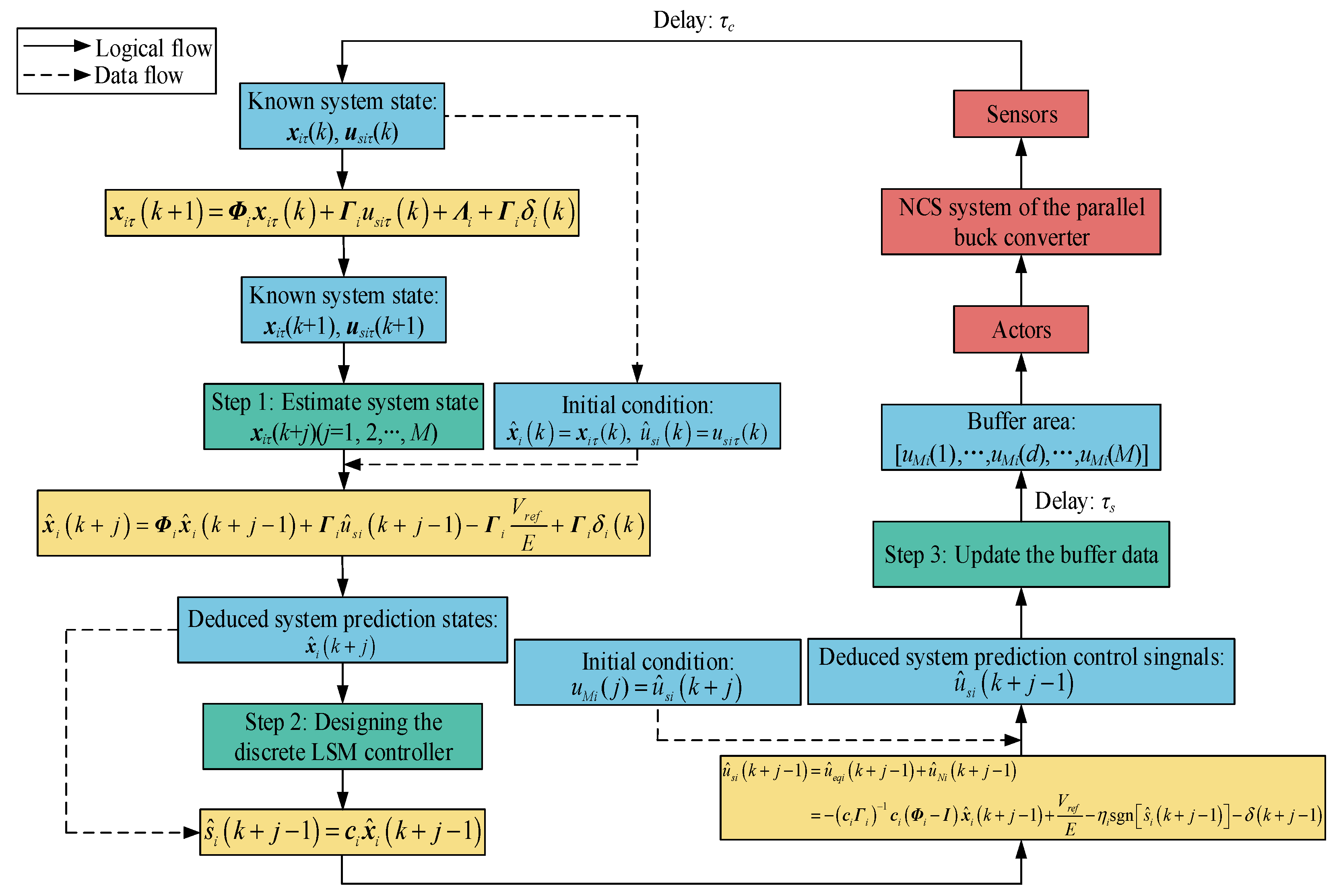
4. Transmission Delay Compensation Strategy Based on Multi-Step Prediction Method

Based on the analysis above, it can be concluded that while the impact of short delays can be negligible, long delays significantly deteriorate the steady-state performance of the NCS. To mitigate this issue, this study proposes a multi-step prediction method with SMC to analyze the current system state and predict the system state backwards in multiple sampling periods. By doing so, the lost control signal because of transmission delay can be compensated, ensuring the desired output performance of the system.

4.1. Design of the Sliding Mode Controller Based on Multi-Step Prediction Method

For bounded delay τ (τ > h), which can be expressed as a multiple of sampling period h relations, i.e., τ = (d’ + l)h, where the d’ ∈ [1, M − 1] ∈ N⁺, l ∈ [0, 1) and M is the upper limit positive integers of (d’ + l). Due to the random variation in l, τ is not always an integer multiple of h. To simplify the analysis and design, this study compensates l to 1, resulting in τ = dh, where d ∈ [2, M] ∈ N⁺. It should be noted that this compensation for l does not significantly alter the original influence of long delay τ on the system, as shown in Figure 3. Therefore, the discrete model of the system in (13) can be re-expressed as:

$${\mathit{x}}_{i\tau }\left(k+1\right)={\mathit{\Phi }}_i{\mathit{x}}_{i\tau }\left(k\right)+{\mathit{\Gamma }}_i{u}_{si\tau }\left(k-d\right)-{\mathit{\Gamma }}_i\frac{V_{ref}}{E}+{\mathit{\Gamma }}_i{\delta }_i\left(k\right)$$

(23)

The delay compensation of the system will be realized based on the multi-step prediction method, and its specific working principle is shown in Figure 4 below:

As shown in Figure 4, since the upper bound of the NCS signal transmission delay is Mh, a buffer u_Mi = [u_Mi(1), u_Mi(2), ⋯, u_Mi(d), ⋯, u_Mi(M)] of length M can be added in front of the actuator to store the pre-predicted control quantity u_si, and the initial value of all elements in u_Mi is zero. By sampling the system output signal every single sampling period h, the obtained sampled data x_iτ(k) is sent to the LSM controller by the transmission delay τ_c; the designed LSM controller generates control signal packet u_si(k + p)(p = 1, 2, ⋯, M) according to the current system state x_iτ(k) prediction; after the u_si(k + p) enters the buffer after the transmission delay τ_s, and is loaded into the corresponding u_Mi in order to be stored, and then the required u_Mi(d) is transmitted to the actuator after the delayed judgment, so as to complete the effective compensation of the system transmission delay within the current h sampling period. It is worth noting that when the packet or actual sample data x_i(k) = [x_1i(t), x_2i(t)]^T with v_Oτ, cannot be updated in real-time due to the delay τ_c greater than h, the buffer will transmit the control signal u_Mi(d + q) to the actuator in order, where q represents the integer quotient of τ_c divided by h, so as to achieve uninterrupted sequential compensation control.

Remark 3.

It should be noted here that in the multi-step prediction-based the NCS shown in Figure 4, both τ_c and τ_s are taken into account in the feedback system. The relationship between τ_c and h directly influences the state of the control signal compensated to the system actuator, while the size of τ_c and τ_s jointly affects the determination of the upper limit of the transmission delay M. This paper determines whether τ_c is greater than h by evaluating the equality of system states x_iτ(k) and x_iτ(k + 1), which cleverly takes the advantage of the fact that when τ_c > h, sensors will transmit the system state saved at the last time when the next sampling time h arrives, avoiding the trouble caused by the delay monitoring of the NCS.

Based on the analysis mentioned above, the crucial step for the compensation system to uphold its efficient output lies in acquiring the buffer control amount u_Mi. Hence, the subsequent paragraphs will outline the entire design procedure for the sliding mode controller based on the prediction method, which is shown in Figure 5.

Step 1: Estimate system state x_iτ(k + j)(j = 1, 2, ⋯, M) based on sampled data x_iτ(k).

In the discrete model of (13), when x_iτ(k) and u_siτ(k) are known, x_i(k + 1) and u_siτ(k + 1) can be obtained. In this way, the system state prediction formula can be designed as

$${\hat{\mathit{x}}}_i\left(k+j\right)={\mathit{\Phi }}_i{\hat{\mathit{x}}}_i\left(k+j-1\right)+{\mathit{\Gamma }}_i{\hat{u}}_{si}\left(k+j-1\right)-{\mathit{\Gamma }}_i\frac{V_{ref}}{E}+{\mathit{\Gamma }}_i{\delta }_i\left(k\right)$$

(24)

where ${\hat{\mathit{x}}}_i\left(k+j\right)$ is the estimated value of system state x_iτ(k + j) after the j-th sampling period predicted by state x_iτ(k), and there is ${\hat{\mathit{x}}}_i\left(k\right)$ = x_iτ(k); ${\hat{u}}_{si}\left(k+j-1\right)$ is the control signal corresponding to the predicted state and satisfying ${\hat{u}}_{si}\left(k\right)$ = u_siτ(k). Since the M times sampling period needs to be estimated backwards, the number of elements ${\hat{u}}_{si}$ is M, and the initial value of each element is zero. For ${\hat{\mathit{x}}}_i\left(k\right)$ = x_iτ(k) and ${\hat{u}}_{si}\left(k\right)$ = u_siτ(k), this will be further explained later in terms of estimated errors. In the process of algorithm implementation, by using the iterative relationship shown in (24), the predicted state ${\hat{\mathit{x}}}_i\left(k+j\right)$ of the system at the next time can be obtained to acquire the system-predicted control signal ${\hat{u}}_{si}\left(k+j-1\right)$.

Step 2: Discrete the LSM controller is designed based on the predicted state.

As seen from (24), in order to obtain ${\hat{\mathit{x}}}_i\left(k+j\right)$, the control signal ${\hat{u}}_{si}\left(k+j-1\right)$ must be obtained first. The discrete LSM surface corresponding to a can be obtained from (14) that:

$${\hat{s}}_i\left(k+j-1\right)={\mathit{c}}_i{\hat{\mathit{x}}}_i\left(k+j-1\right)$$

(25)

By substituting (15) and (16) into (25), the equivalent control law ${\hat{u}}_{eqi}\left(k+j\right)$ and ${\hat{u}}_{Ni}\left(k+j\right)$ the switching control law can be obtained respectively as:

$${\hat{u}}_{eqi}\left(k+j-1\right)=-{\left({\mathit{c}}_i{\mathit{\Gamma }}_i\right)}^{-1}{\mathit{c}}_i\left({\mathit{\Phi }}_i-\mathit{I}\right){\hat{\mathit{x}}}_i\left(k+j-1\right)+\frac{V_{ref}}{E}-\delta \left(k+j-1\right)$$

(26)

$${\hat{u}}_{Ni}\left(k+j-1\right)=-{\eta }_i\mathrm{sgn}\left[{\hat{s}}_i\left(k+j-1\right)\right]$$

(27)

The control law ${\hat{u}}_{si}\left(k+j-1\right)$ can be further obtained by combining (25) and (26) as:

$$\begin{array}{cc}\hfill {\hat{u}}_{si}\left(k+j-1\right)& ={\hat{u}}_{eqi}\left(k+j-1\right)+{\hat{u}}_{Ni}\left(k+j-1\right)\hfill \\ & =-{\left({\mathit{c}}_i{\mathit{\Gamma }}_i\right)}^{-1}{\mathit{c}}_i\left({\mathit{\Phi }}_i-\mathit{I}\right){\hat{\mathit{x}}}_i\left(k+j-1\right)+\frac{V_{ref}}{E}-{\eta }_i\mathrm{sgn}\left[{\hat{s}}_i\left(k+j-1\right)\right]-\delta \left(k+j-1\right)\hfill \end{array}$$

(28)

Therefore, after x_iτ(k) is obtained from each sampling period, ${\hat{u}}_{si}\left(k+j-1\right)$ and ${\hat{\mathit{x}}}_{i\tau }\left(k+j\right)$ in the following M sampling periods can be predicted by steps 1 and 2 respectively, ${\hat{u}}_{si}\left(k+j-1\right)$ can also be turned into a switching signal ${\hat{u}}_i\left(k+j-1\right)$ by PWM as shown in (10). Hence, the predicted control signals in the controller buffer are continuously supplemented.

Step 3: Update the buffer data with predictive control signals.

The M predictive control signals obtained in step 2 are arranged in sequence and sent to the buffer in a unified package to update the data in u_Mi, that is, u_Mi(j) = ${\hat{u}}_{si}\left(k+j\right)$. After that, the system will select the corresponding u_Mi(d) according to the measured system transmission delay τ and send it to the actuator. If the data in the buffer is not updated and the next sampling period has been entered at this time, the system will successively send u_Mi(d + 1) and subsequent control signals in the buffer to the actuator to ensure the continuity of the output signals of the controller, and the converter maintains stable operation; if the buffer has been updated, repeat step 3.

By repeating the above steps according to the sampling time h, the transmission delay of the NCS signal in the parallel buck converter can be compensated.

4.2. System Stability Analysis

The approach proposed in this paper aims to use the current system state for predicting future state quantities, enabling the proactive acquisition of corresponding control quantities to compensate for signal transmission delays. Thus, the crucial aspect of analyzing system stability lies in evaluating the accuracy of these predictions. This paper introduces an error variable following, which indicates the discrepancy between the estimated value and the actual value of the subsequent system:

$${\mathit{e}}_i(j)={\mathit{x}}_{i\tau }(k+j)-{\hat{\mathit{x}}}_i(k+j)$$

(29)

where e_i(j) represents the deviation between the actual state value of the system and the true state value. And the expression of x_iτ(k + j) can be obtained from (13) as:

$${\mathit{x}}_{i\tau }\left(k+j\right)={\mathit{\Phi }}_i{\mathit{x}}_{i\tau }\left(k+j-1\right)+{\mathit{\Gamma }}_i{u}_{si\tau }\left(k+j-1\right)-{\mathit{\Gamma }}_i\frac{V_{ref}}{E}+{\mathit{\Gamma }}_i{\delta }_i\left(k+j-1\right)$$

(30)

Further substitute (24) and (30) into Equation (29) to obtain:

$$\begin{array}{cc}\hfill {\mathit{e}}_i(j)& ={\mathit{\Phi }}_i^j{\mathit{x}}_{i\tau }(k)+{\mathit{\Phi }}_i^{(j-1)}{\mathit{\Gamma }}_i{u}_{si}(k)+\cdots +{\mathit{\Phi }}_i{\mathit{\Gamma }}_i{u}_{si}(k+j-2)+{\mathit{\Gamma }}_i{u}_{si}(k+j-1)+{\mathit{\Phi }}_i{}^{(j-1)}{\mathit{\Gamma }}_i{\mathit{\delta }}_i(k)+\cdots +{\mathit{\Phi }}_i{\mathit{\Gamma }}_i{\delta }_i(k+j-2)\hfill \\ & +{\mathit{\Gamma }}_i{\delta }_i(k+j-1)-{\mathit{\Phi }}_i^j{\mathit{x}}_{i\tau }(k)-{\mathit{\Phi }}_i^{(j-1)}{\mathit{\Gamma }}_i{u}_{si}(k)-\cdots -{\mathit{\Phi }}_i{\mathit{\Gamma }}_i{\hat{u}}_{si}(k+j-2)-{\mathit{\Gamma }}_i{\hat{u}}_{si}(k+j-1)\hfill \\ & ={\displaystyle \sum _{q=0}^{j-1}{\mathit{\Phi }}_i^q{\mathit{\Gamma }}_i{\delta }_i(k+j-1-q)}\hfill \end{array}$$

(31)

According to the design idea of the buffer, its memory length should meet M ≥ d. Since d is constant, the control signal predicted by the sampled system state x_iτ(k) is ${\hat{u}}_{si}\left(k+d\right)$, which corresponds to the LSM surface ${\hat{s}}_i\left(k+d\right)$. The Lyapunov equation can also be designed as:

$${\hat{V}}_i\left(k+d\right)={\hat{s}}_i^2\left(k+d\right)$$

(32)

According to the stability conditions of the discrete LSMC system, in order to ensure the stability of the multi-step predictive control system, (32) must meet the following conditions:

$$\Delta {\hat{V}}_i\left(k+d\right)={\hat{V}}_i\left(k+d+1\right)-{\hat{V}}_i\left(k+d\right)={\hat{s}}_i{}^2\left(k+d+1\right)-{\hat{s}}_i{}^2\left(k+d\right)<0$$

(33)

For ease of analysis, Equation (32) can be further rewritten as:

$$\Delta {\hat{V}}_i\left(k+d\right)={\left[{\hat{s}}_i\left(k+d+1\right)-{\hat{s}}_i\left(k+d\right)\right]}^2+2{\hat{s}}_i\left(k+d\right)\left[{\hat{s}}_i\left(k+d+1\right)-{\hat{s}}_i\left(k+d\right)\right]<0$$

(34)

Let $\Delta {\hat{s}}_i\left(k+d\right)={\hat{s}}_i\left(k+d+1\right)-{\hat{s}}_i\left(k+d\right)$, then from (24) to (29) we can get:

$$\begin{array}{cc}\hfill \Delta {\hat{s}}_i\left(k+d\right)& ={\hat{s}}_i\left(k+d+1\right)-{\hat{s}}_i\left(k+d\right)={\mathit{c}}_i{\hat{\mathit{x}}}_i\left(k+d+1\right)-{\mathit{c}}_i{\hat{\mathit{x}}}_i\left(k+d\right)\hfill \\ & ={\mathit{c}}_i{\mathit{\Phi }}_i{\mathit{e}}_i\left(d\right)-{\mathit{c}}_i{\mathit{e}}_i\left(d+1\right)+{\mathit{c}}_i{\mathit{\Gamma }}_i{\hat{u}}_{Ni}\left(k+d\right)+{\mathit{c}}_i{\mathit{\Gamma }}_i{\delta }_i\left(k+d\right)\hfill \end{array}$$

(35)

By substituting (35) into (34), there is:

$$\begin{array}{ll}\hfill \Delta {\hat{V}}_i\left(k+d\right)& =\Delta {\hat{s}}_i{\left(k+d\right)}^2+2{\hat{s}}_i\left(k+d\right)\Delta {\hat{s}}_i\left(k+d\right)\hfill \\ & ={\left[{\mathit{c}}_i{\mathit{\Phi }}_i{\mathit{e}}_i\left(d\right)-{\mathit{c}}_i{\mathit{e}}_i\left(d+1\right)+{\mathit{c}}_i{\mathit{\Gamma }}_i{\hat{u}}_{Ni}\left(k+d\right)+{\mathit{c}}_i{\mathit{\Gamma }}_i{\delta }_i\left(k+d\right)\right]}^2\hfill \\ & +2{\hat{s}}_i\left(k+d\right)\left[{\mathit{c}}_i{\mathit{\Phi }}_i{\mathit{e}}_i\left(d\right)-{\mathit{c}}_i{\mathit{e}}_i\left(d+1\right)+{\mathit{c}}_i{\mathit{\Gamma }}_i{\hat{u}}_{Ni}\left(k+d\right)+{\mathit{c}}_i{\mathit{\Gamma }}_i{\delta }_i\left(k+d\right)\right]<0\hfill \end{array}$$

(36)

In (36), without considering ${\hat{s}}_i\left(k+d\right)=0$, it can be divided into ${\hat{s}}_i\left(k+d\right)>0$ and ${\hat{s}}_i\left(k+d\right)<0$ to discuss system stability:

(1)

When ${\hat{s}}_i\left(k+d\right)>0$, from (36) we can get:

$$\begin{array}{ll}\hfill \Delta {\hat{V}}_i\left(k+d\right)& =\Delta {\hat{s}}_i{\left(k+d\right)}^2+2{\hat{s}}_i\left(k+d\right)\Delta {\hat{s}}_i\left(k+d\right)\hfill \\ & ={\left[{\mathit{c}}_i{\mathit{\Phi }}_i{\mathit{e}}_i\left(d\right)-{\mathit{c}}_i{\mathit{e}}_i\left(d+1\right)+{\mathit{c}}_i{\mathit{\Gamma }}_i{\hat{u}}_{Ni}\left(k+d\right)+{\mathit{c}}_i{\mathit{\Gamma }}_i{\delta }_i\left(k+d\right)\right]}^2\hfill \\ & +2{\hat{s}}_i\left(k+d\right)\left[{\mathit{c}}_i{\mathit{\Phi }}_i{\mathit{e}}_i\left(d\right)-{\mathit{c}}_i{\mathit{e}}_i\left(d+1\right)+{\mathit{c}}_i{\mathit{\Gamma }}_i{\hat{u}}_{Ni}\left(k+d\right)+{\mathit{c}}_i{\mathit{\Gamma }}_i{\delta }_i\left(k+d\right)\right]\hfill \\ & \le {\left[{\displaystyle \sum _{q=0}^{d-1}\left|{\mathit{c}}_i{\mathit{\Phi }}_i^{\left(q+1\right)}{\mathit{\Gamma }}_i{\beta }_i\right|}-{\displaystyle \sum _{p=0}^d\left|{\mathit{c}}_i{\mathit{\Phi }}_i^p{\mathit{\Gamma }}_i{\beta }_i\right|+\left|{\mathit{c}}_i{\mathit{\Gamma }}_i{\beta }_i\right|+{\mathit{c}}_i{\mathit{\Gamma }}_i{\hat{u}}_{Ni}\left(k+d\right)}\right]}^2\hfill \\ & +2{\hat{s}}_i\left(k+d\right)\left[{\displaystyle \sum _{q=0}^{d-1}\left|{\mathit{c}}_i{\mathit{\Phi }}_i^{\left(q+1\right)}{\mathit{\Gamma }}_i{\beta }_i\right|}\right.\left.-{\displaystyle \sum _{p=0}^d\left|{\mathit{c}}_i{\mathit{\Phi }}_i^p{\mathit{\Gamma }}_i{\beta }_i\right|}+\left|{\mathit{c}}_i{\mathit{\Gamma }}_i{\beta }_i\right|+{\mathit{c}}_i{\mathit{\Gamma }}_i{\hat{u}}_{Ni}\left(k+d\right)\right]\hfill \\ & ={\left[{\mathit{c}}_i{\mathit{\Gamma }}_i{\hat{u}}_{Ni}\left(k+d\right)\right]}^2+2{\hat{s}}_i\left(k+d\right){\mathit{c}}_i{\mathit{\Gamma }}_i{\hat{u}}_{Ni}\left(k+d\right)<0\hfill \end{array}$$

(37)

Since ${\hat{s}}_i\left(k+d\right)>0$, in order to ensure that the relationship in (36) holds, the parameters of the control system need to meet the following conditions:

$$\left\{\begin{array}{l}{\mathit{c}}_i{\mathit{\Gamma }}_i{\hat{u}}_{Ni}\left(k+d\right)<0\\ 2{\hat{s}}_i\left(k+d\right)>-{\mathit{c}}_i{\mathit{\Gamma }}_i{\hat{u}}_{Ni}\left(k+d\right)\end{array}\right.$$

(38)

By substituting (27) into (38), (38) can be rewritten as:

$$\left\{\begin{array}{l}-{\mathit{c}}_i{\mathit{\Gamma }}_i{\eta }_i<0\\ 2{\hat{s}}_i\left(k+d\right)>{\mathit{c}}_i{\mathit{\Gamma }}_i{\eta }_i\end{array}\right.$$

(39)

When the sampling period h meets 0 < h < 2nRC_i, c_iΓ_i > 0 is established by substituting c_i and Γ_i into (39). Since the switching gain η_i > 0, the establishment condition of (39) is

$${\hat{s}}_i\left(k+d\right)>\frac{\left[\frac{Eh}{L_i{C}_i}+\left({\lambda }_i+k_i{S}_{xi}\right)\frac{E{h}^2}{2L_i{C}_i}-\frac{E{h}^2}{2nR{L}_i{C}_i^2}\right]{\eta }_i}{2}$$

(40)

(2)

When ${\hat{s}}_i\left(k+d\right)<0$, from (36) we can also get:

$$\Delta {\hat{V}}_i\left(k+d\right)={\left[{\mathit{c}}_i{\mathit{\Gamma }}_i{u}_{Ni}\left(k+d\right)\right]}^2+2{\hat{s}}_i\left(k+d\right){\mathit{c}}_i{\mathit{\Gamma }}_i{\hat{u}}_{Ni}\left(k+d\right)<0$$

(41)

Given that ${\hat{s}}_i\left(k+d\right)<0$, it is essential to satisfy the following conditions for the parameters of the control system in order to maintain the validity of the relationship expressed in Equation (41):

$$\left\{\begin{array}{l}{\mathit{c}}_i{\mathit{\Gamma }}_i{\hat{u}}_{Ni}\left(k+d\right)>0\\ 2{\hat{s}}_i\left(k+d\right)<-{\mathit{c}}_i{\mathit{\Gamma }}_i{\hat{u}}_{Ni}\left(k+d\right)\end{array}\right.$$

(42)

And (42) can be rewritten as follows by further substituting (27) into it:

$$\left\{\begin{array}{l}{\mathit{c}}_i{\mathit{\Gamma }}_i{\eta }_i>0\\ 2{\hat{s}}_i\left(k+d\right)<-{\mathit{c}}_i{\mathit{\Gamma }}_i{\eta }_i\end{array}\right.$$

(43)

The parameter matrixes c_i and Γ_i can also be substituted into (43) as:

$${\hat{s}}_i\left(k+d\right)<-\frac{\left[\frac{Eh}{L_i{C}_i}+\left({\lambda }_i+k_i{S}_{xi}\right)\frac{E{h}^2}{2L_i{C}_i}-\frac{E{h}^2}{2nR{L}_i{C}_i^2}\right]{\eta }_i}{2}$$

(44)

According to (40) and (44), the stability condition of the multi-step predictive control system designed in this paper can be expressed as:

$$0<\frac{{\mathit{c}}_i{\mathit{\Gamma }}_i{\eta }_i}{2}<\left|{\hat{s}}_i\left(k+d\right)\right|$$

(45)

From (45), the results show that the system state will eventually converge to the vicinity of the SM surface as:

$$s_i^{\Delta }=\left\{s_i\left(k+j\right)\left|-\frac{{\mathit{c}}_i{\mathit{\Gamma }}_i{\eta }_i}{2}\le {\hat{s}}_i\left(k+d\right)\le \frac{{\mathit{c}}_i{\mathit{\Gamma }}_i{\eta }_i}{2}\right.\right\}$$

(46)

5. Simulation and Experimental Verification

5.1. Simulation Analysis and Verification

The performance of the SMC system designed in this paper will be evaluated through simulations. Specifically, the output current and system control quantity for phase i of the parallel buck converter’s NCS will be investigated. The sampling period is set to h = 0.1 ms, and the controller parameters are set as λ_i = 600, k_i = 100. Random delays τ, ranging from [0, 0.2 ms], [0, 0.4 ms], and [0, 0.6 ms], will be introduced to the NCS, and τ_s and τ_c obtain the delay randomly assigned by τ, while keeping the parameters in Table 1 unchanged. And the random noise disturbance of 0–1 V is superimposed on the input of each phase of the control signal of the buck converter.

Table 3. System performance results before and after delay compensation in different intervals.

τ (ms)	Compensated State	ΔvOτ (V)	ΔvOτ_max (V)	ΔiLiτ (A)	ΔiLiτ_max (A)	System Current Mode
0.2	No	0.22	0.78	1.02	0.44	CCM
	Yes	0.02	0.01	0.81	0.37	CCM
0.4	No	0.31	2.96	1.29	1.01	DCM
	Yes	0.08	1.58	1.03	0.45	CCM
0.6	No	0.35	2.41	1.61	1.39	DCM
	Yes	0.11	1.42	1.38	0.67	CCM

and Figure 6 below show the simulation results before and after processing with the delay signal compensation.

The system output v_Oτ, before and after compensation, under different intervals of long delay are presented in Figure 6a,c,e. When the delay τ falls in [0, 0.2 ms], it can be seen that the compensated v_Oτ is 0.2 V lower than the uncompensated voltage fluctuation, and the dynamic response time of the voltage is nearly 0.01 s higher, and the maximum voltage error Δv_{Oτ_max} is reduced from 0.78 V to 0.01 V by compensation. When the delay τ further increases to the range with [0, 0.4 ms], the uncompensated v_Oτ shows more violent fluctuations, and the steady-state error reached 0.31 V, while the compensated v_Oτ remained stable, with only 0.08 V steady-state error, and the Δv_{Oτ_max} is also reduced 1.38 V. When the τ falls in the range [0, 0.2 ms], it can be seen from the uncompensated v_Oτ that the transmission of the control signal of the system is seriously damaged at this time, and the Δv_Oτ and Δv_{Oτ_max} reach 0.35 V and 2.41 V, respectively. However, they can be reduced by 0.24 V and 0.99 V through compensation, so that the voltage curve can remain stable, which also evidences that the addition of multi-step predictive control significantly reduces the fluctuation range of the output voltage and current, leading to a more stable system output.

Figure 6b,d,f show the system output current signal i_Liτ before and after compensation. With the increase in the system transmission signal delay τ, the fluctuation steady-state error Δi_Liτ of the uncompensated signal i_Liτ increases from 1.02 A to 1.61 A, and the maximum current error Δi_{Liτ_max} increases from 0.44 A to 1.39 A, almost doubling the rated current value, the i_Liτ also changes from CCM to DCM. While the fluctuating peak current will cause damage to the stability of the converter load. After the compensation controller is added, it can be seen that the Δi_Liτ decreases by 0.21 A, 0.26 A and 0.23 A, respectively, and the Δi_{Liτ_max} decreases by 0.07 A, 0.56 A, and 0.72 A, respectively, and the current stability increases significantly. It can further be observed that the enhanced NCS leads to the system output i_Liτ operating under CCM, which is attributed to the effective compensation of the multi-step predictive controller for losing the system control signal caused by delays.

Figure 6h visually confirms the continuity of the system control signal u_si. It can be observed that with the increase in system transmission delay τ, u_si gradually fluctuates, but it can remain continuous and stable under the compensation of the multiple unpredictable controller. When the τ reaches 4 times and 6 times the sampling time h, u_si can already remain near 0.5 in the initial 0.5 s to maintain the stable operation of the system. The improvement effectively mitigates the impact of long delays on system output performance, further enhancing the steady-state output performance of the parallel buck converter system.

Figure 6g demonstrates the sliding variable s_i of the system with different time delays after compensation. Thanks to the multi-step predictive controller, s_i maintains both continuity and stability despite delays. This not only leverages the characteristics of SMC but also ensures the system’s strong robustness.

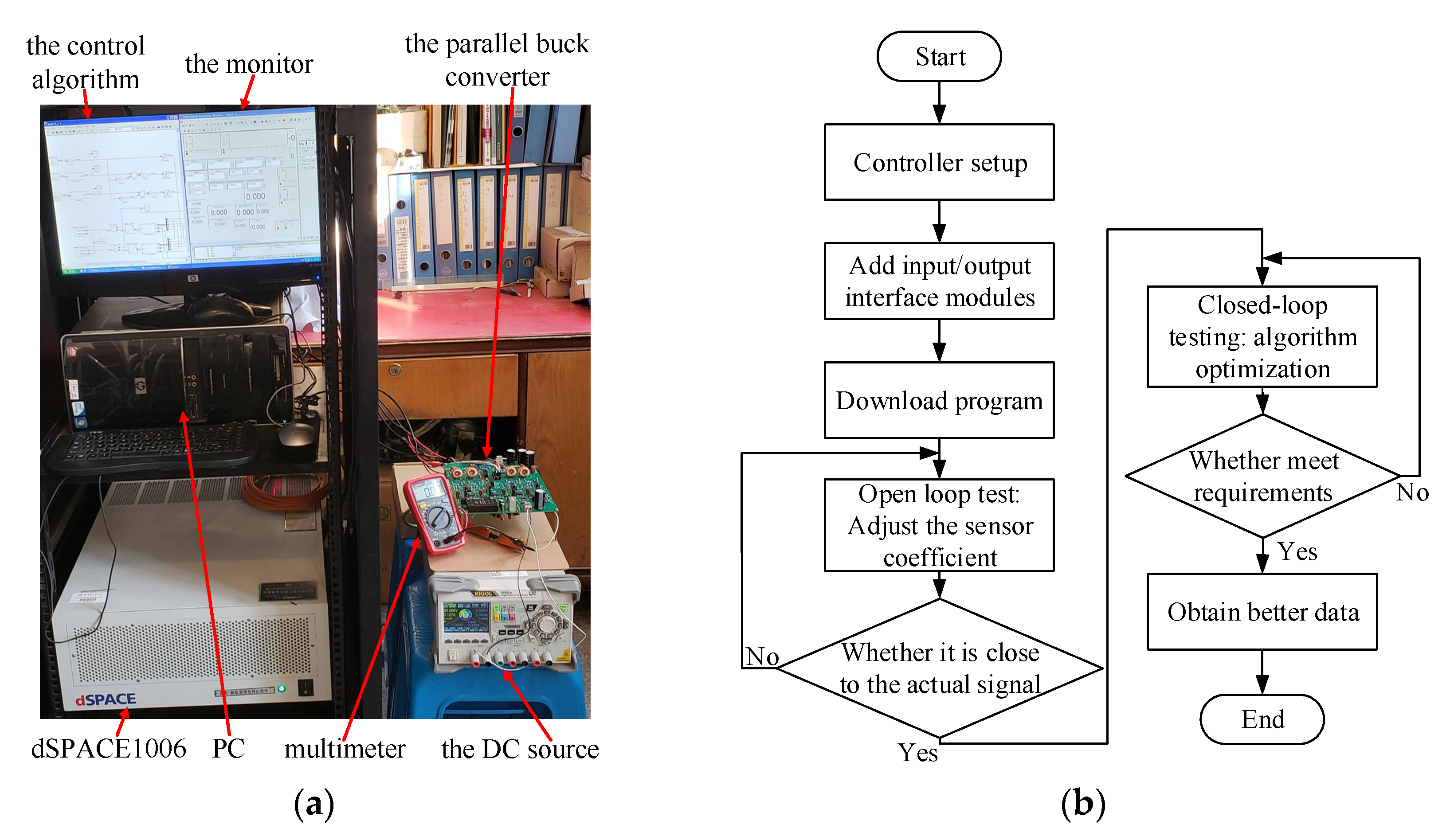
5.2. Experimental Verification

In this paper, the dSPACE1006 controller with powerful data computing capability is selected to verify the designed control strategy and some theories. The experimental platform of the parallel buck converter control system based on dSPACE1006 is established as shown in Figure 7a, and its operating process is illustrated in Figure 7b.

5.2.1. Verification of the Effect of Different Delays on NCS’s Output Performance

Keep the converter circuit parameters consistent with those in Table 1. And the controller parameter λ_i = 600, k_i = 100 and the sampling period h = 0.1 ms are set unchanged, so that the signal transmission delay is within four random intervals of [0, 0.1 ms], [0, 0.2 ms], [0, 0.4 ms] and [0, 0.6 ms], respectively. The experimental results are shown in

Table 4. System output voltage characteristics under different time delays.

τ (ms)	Rise Time (ms)	Mean Steady-State Error (V)	Maximum Amplitude Error (V)
0	103	0.22	0.37
0–0.1	122	0.40	0.50
0–0.2	138	0.74	1.01
0–0.4	148	0.89	1.41
0–0.6	173	0.91	1.61

and Figure 8 below.

The output voltage v_Oτ shown in Figure 8a demonstrates that the presence of random delays in the NCS has minimal impact on the output voltage characteristics when the delay is equal to or less than one sampling period. Thus, the effect of this delay type on the system performance can be disregarded. However, further examination of Figure 8b–d and Table 4 reveals that as the transmission delay increases, both the rise time and the maximum error of the system output voltage increase. Precisely, when the random delay ranges from 0 to 0.2 ms, 0 to 0.4 ms, and 0 to 0.6 ms, the maximum error corresponds to values of 0.74 V, 0.89 V, and 0.91 V, respectively. These results indicate a poor steady-state performance that fails to meet the required performance standards, necessitating the implementation of delayed compensation processing. The experimental findings confirm that short delays have a negligible impact on the NCS performance, while longer delays adversely affect both the transient and steady-state performance of the control system and increase the steady-state error. These conclusions align with the outcome of the simulation analysis obtained in Figure 3.

5.2.2. Verification of Compensation Strategy for NCS Transmitted Delay Signal Based on Multi-Step Prediction Method

As seen from Figure 8 and Table 4, performing the control system with random delays of [0, 0.4 ms] and [0, 0.6 ms] is poor, hence, it is very important to compensate the long transmission delay of the NCS in the parallel buck converter, which is one of the important conclusions of this paper. The actual compensation effect of the LSM controller designed in this paper based on the multi-step prediction method to the long transmission delay of the system NCS will be verified by designed experiments.

Similarly, the 0–1 V random noise disturbance signal is superimposed on the input side of each phase control signal of the parallel buck converter. Here, typical random long transmission delay intervals [0, 0.4 ms] and [0, 0.6 ms] shown in Figure 8c,d are selected to verify the effectiveness of the designed controller, and the experimental results are shown in

Table 5. The output voltage characteristics before and after treatment with the multi-step prediction method.

τ (ms)	Compensated State	Rise Time (ms)	Mean Steady-State Error (V)	Maximum Amplitude Error (V)
0–0.4	No	148	0.89	0.99
	Yes	64	0.48	0.78
0–0.6	No	173	0.91	1.39
	Yes	67	0.57	0.62

and Figure 9.

As evidenced by the output voltage v_Oτ presented in Figure 9 and the accompanying data in Table 5, both the buffer method and the multi-step prediction method effectively mitigate the adverse impact of signal transmission delay on the steady-state performance of NCS. This mitigation is reflected in a substantial reduction in the maximum error in the system’s output voltage, from 0.89 V and 0.91 V to 0.48 V and 0.57 V, respectively, resulting in a marked improvement in steady-state performance. Following implementing delay compensation, the rise time of the system’s output voltage decreases from 148 ms and 173 ms to 64 ms and 67 ms, respectively, signifying a noticeable enhancement in system response speed. It is worth noting that the system experiences an overshoot phenomenon, with overshoot values of 0.48 V and 0.57 V, respectively, because of employing advanced prediction techniques, which have a detrimental effect on transient performance. An examination of the output voltage waveform reveals sporadic occurrences of minor peaks during the steady-state phase. This observation underscores certain limitations in the multi’s utilization-step prediction method for delay compensation.

6. Conclusions

In this paper, the effect of random long delay on the NCS performance of the parallel buck converter system is analyzed in detail. The results show that the effect of short delays on the system can be ignored, but long delays will increase the steady-state error of the system output and seriously affect the system’s stability. Therefore, this paper proposes a sliding mode control strategy based on the multi-step prediction method. Firstly, the discrete domain model of the system and the LSM controller are constructed and constructed. On this basis, the influence of long delay and matching disturbance on the NCS is fully considered, and the compensation strategy of the multi-step prediction method is designed. Through the continuous supply of the predictive control quantity stored in the buffer, losing the NCS control signal in the case of long delays is compensated, thus easing the impact of signal transmission delay on the system performance and ensuring the stability of the system output. Finally, the multi-step predictive control strategy proposed in this paper demonstrates remarkable improvements in system performance through the designed experiments. On average, this strategy reduces the system’s output steady-state error by 41.6%, while also reducing the output response time by 61.2% and the maximum error of the output signal by 20.6%. These significant improvements clearly validate the superiority of the proposed method, which proves the correction of the proposed method.

References

1. Peng, D.; Huang, M.; Li, J.; Sun, J.; Zha, X.; Wang, C. Large-signal stability criterion for parallel-connected DC–DC converters with current source equivalence. IEEE Trans. Circuits Syst. II Express Briefs 2019, 66, 2037–2041. [Google Scholar] [CrossRef]
2. Li, H.; Ren, F.; Liu, C.; Guo, Z.; Lü, J.; Zhang, B.; Zheng, T.Q. An extended stability analysis method for paralleled dc-dc converters system with considering the periodic disturbance based on floquet theory. IEEE Access 2020, 8, 9023–9036. [Google Scholar] [CrossRef]
3. Shi, J.; Zhou, L.; Li, J.; He, X. Common-duty-ratio control of input-parallel output-parallel (IPOP) connected DC–DC converter modules with automatic sharing of currents. IEEE Trans. Power Electron. 2012, 27, 3277–3291. [Google Scholar] [CrossRef]
4. Panov, Y.; Jovanovic, M.M. Loop gain measurement of paralleled DC–DC converters with average-current-sharing control. IEEE Trans. Power Electron. 2008, 23, 2942–2948. [Google Scholar] [CrossRef]
5. Xu, G.; Sha, D.; Liao, X. Decentralized inverse-droop control for input-series–output-parallel DC–DC converters. IEEE Trans. Power Electron. 2015, 30, 4621–4625. [Google Scholar] [CrossRef]
6. Wang, R.; Liu, G.-P.; Wang, J.; Rees, D.; Zhao, Y.B. Guaranteed cost control for networked control systems based on an improved predictive control method. IEEE Trans. Control Syst. Technol. 2010, 18, 1226–1232. [Google Scholar] [CrossRef]
7. Klügel, M.; Mamduhi, M.; Ayan, O.; Vilgelm, M.; Johansson, K.H.; Hirche, S.; Kellerer, W. Joint cross-layer optimization in real-time networked control systems. IEEE Trans. Control Netw. Syst. 2020, 7, 1903–1915. [Google Scholar] [CrossRef]
8. Zhao, Y.-B.; Liu, G.-P.; Rees, D. Design of a packet-based control framework for networked control systems. IEEE Trans. Control Syst. Technol. 2009, 17, 859–865. [Google Scholar] [CrossRef]
9. Wu, C.; Liu, J.; Jing, X.; Li, H.; Wu, L. Adaptive fuzzy control for nonlinear networked control systems. IEEE Trans. Syst. Man Cybern. Syst. 2017, 47, 2420–2430. [Google Scholar] [CrossRef]
10. Xu, H.; Jagannathan, S. Neural network-based finite horizon stochastic optimal control design for nonlinear networked control systems. IEEE Trans. Neural Netw. Learn. Syst. 2015, 26, 472–485. [Google Scholar] [CrossRef]
11. Shi, Y.; Yu, B. Output feedback stabilization of networked control systems with random delays modeled by markov chains. IEEE Trans. Autom. Control 2009, 54, 1668–1674. [Google Scholar]
12. Qiu, J.; Gao, H.; Ding, S.X. Recent advances on fuzzy-model-based nonlinear networked control systems: A survey. IEEE Trans. Ind. Electron. 2016, 63, 1207–1217. [Google Scholar] [CrossRef]
13. Tavassoli, B. Stability of nonlinear networked control systems over multiple communication links with asynchronous sampling. IEEE Trans. Autom. Control 2014, 59, 511–515. [Google Scholar] [CrossRef]
14. Savkin, A.V.; Cheng, T.M. Detectability and output feedback stabilizability of nonlinear networked control systems. IEEE Trans. Autom. Control 2007, 52, 730–735. [Google Scholar] [CrossRef]
15. Liu, K.-Z.; Wang, R.; Liu, G.-P. Tradeoffs between transmission intervals and delays for decentralized networked control systems based on a gain assignment approach. IEEE Trans. Circuits Syst. II Express Briefs 2016, 63, 498–502. [Google Scholar] [CrossRef]
16. Maity, D.; Mamduhi, M.H.; Hirche, S.; Johansson, K.H. Optimal lqg control of networked systems under traffic-correlated delay and dropout. IEEE Control Syst. Lett. 2022, 6, 1280–1285. [Google Scholar] [CrossRef]
17. Tang, B.; Wang, J.; Zhang, Y. A delay-distribution approach to stabilization of networked control systems. IEEE Trans. Control Netw. Syst. 2015, 2, 382–392. [Google Scholar] [CrossRef]
18. Tan, C.; Zhang, H. Necessary and sufficient stabilizing conditions for networked control systems with simultaneous transmission delay and packet dropout. IEEE Trans. Autom. Control 2017, 62, 4011–4016. [Google Scholar] [CrossRef]
19. Shangguan, X.-C.; Zhang, C.-K.; He, Y.; Jin, L.; Jiang, L.; Spencer, J.W.; Wu, M. Robust load frequency control for power system considering transmission delay and sampling period. IEEE Trans. Ind. Inform. 2021, 17, 5292–5303. [Google Scholar] [CrossRef]
20. Pang, H.-p.; Liu, C.-j.; Liu, A.-z. Sliding Mode Control for Time-DELAY systems with Its Application to Networked Control Systems. In Proceedings of the Sixth International Conference on Intelligent Systems Design and Applications, Jian, China, 16–18 October 2006; pp. 192–197. [Google Scholar]
21. Yan, S.; Shen, M.Q.; Nguang, S.K.; Zhang, G.M. Event-triggered H∞ control of networked control systems with distributed transmission delay. IEEE Trans. Autom. Control 2020, 65, 4295–4301. [Google Scholar] [CrossRef]
22. Kim, D.S.; Choi, D.H.; Mohapatra, P. Real-time scheduling method for networked discrete control systems. Control Eng. Pract. 2009, 17, 564–570. [Google Scholar] [CrossRef]
23. Heemels, W.P.M.H.; Teel, A.R.; van de Wouw, N.; Nesic, D. Networked control systems with communication constraints: Tradeoffs between transmission intervals, delays and performance. IEEE Trans. Autom. Control 2010, 55, 1781–1796. [Google Scholar] [CrossRef]
24. Padhy, B.P.; Srivastava, S.C.; Verma, N.K. A Wide-Area Damping Controller Considering Network Input and Output Delays and Packet Drop. IEEE Trans. Power Syst. 2017, 32, 166–176. [Google Scholar] [CrossRef]
25. Liu, G.P.; Chai, S.C.; Mu, J.X.; Rees, D. Networked Predictive Control of Systems with Random Delay in Signal Transmission Channels. Int. J. Syst. Sci. 2008, 39, 1055–1064. [Google Scholar] [CrossRef]
26. Huangfu, Y.; Ma, R.; Zhao, B.; Liang, Z.; Ma, Y.; Wang, A.; Zhao, D.; Li, H.; Ma, R. A novel robust smooth control of input parallel output series quasi-z-source DC–DC converter for fuel cell electrical vehicle applications. IEEE Trans. Ind. Appl. 2021, 57, 4207–4221. [Google Scholar] [CrossRef]
27. Mosayebi, M.; Gheisarnejad, M.; Khooban, M.H. An intelligent sliding mode control for stabilization of parallel converters feeding cpls in DC-microgrid. IET Power Electron. 2022, 15, 1596–1606. [Google Scholar] [CrossRef]
28. Lee, S.; Jeung, Y.-C.; Lee, D.-C. Voltage balancing control of ipos modular dual active bridge DC/DC converters based on hierarchical sliding mode control. IEEE Access 2019, 7, 9989–9997. [Google Scholar] [CrossRef]
29. Wei, Z.; Zhang, W.; Wang, Y. Sliding mode control for parallel DC–DC converter network systems with uniform quantization and discretization effects. IEEE Access 2023, 11, 99918–99934. [Google Scholar] [CrossRef]
30. Lopez, M.; Vicuna, L.G.; Castilla, M.; Gaya, P.; Lopez, O. Current distribution control design for paralleled DC/DC converters using sliding-mode control. IEEE Trans. Ind. Electron. 2004, 51, 419–428. [Google Scholar] [CrossRef]
31. Taheri, B.; Sedaghat, M.; Bagherpour, M.A.; Farhadi, P. A New Controller for DC-DC Converters Based on Sliding Mode Control Techniques. J. Control. Autom. Electr. Syst. 2019, 30, 63–74. [Google Scholar] [CrossRef]
32. Alsmadi, Y.; Utkin, V.; Haj-ahmed, M.; Xu, L. Sliding mode control of power converters: DC/DC converters. Int. J. Control 2018, 91, 2472–2493. [Google Scholar] [CrossRef]
33. Zhao, Y.; Qiao, W.; Ha, D. A sliding-mode duty-ratio controller for DC/DC buck converters with constant power loads. IEEE Trans. Ind. Appl. 2014, 50, 1448–1458. [Google Scholar] [CrossRef]
Figure 1. An NCS with transmission delays of the n-phase parallel buck converter.
Electronics 13 00121 g001
Figure 2. System output performances in random short delay interval: (a) v in 0.05 ms delay; (b) iLiτ in 0.05 ms delay; (c) v in 0.1 ms delay; (d) iLiτ in 0.1 ms delay.
Electronics 13 00121 g002aElectronics 13 00121 g002b
Figure 3. System output performances in random long delay interval: (a) v in 0.2 ms delay; (b) iLiτ in 0.2 ms delay; (c) v in 0.4 ms delay; (d) iLiτ in 0.4 ms delay; (e) v in 0.6 ms delay; (f) iLiτ in 0.6 ms delay.
Electronics 13 00121 g003
Figure 4. NCS signal transmission process based on multi-step prediction method.
Electronics 13 00121 g004
Figure 5. Design flow chart of the LSM controller based on multi-step prediction method.
Electronics 13 00121 g005
Figure 6. The output performance of NCS before and after compensation under different delays: (a) v in 0.2 ms delay; (b) iLiτ in 0.2 ms delay; (c) v in 0.4 ms delay; (d) iLiτ in 0.4 ms delay; (e) v in 0.6 ms delay; (f) iLiτ in 0.6 ms delay; (g) si in long delays; (h) usi in long delays.
Electronics 13 00121 g006
Figure 7. Illustration of the experimental platform based on the dSPACE1006: (a) experimental platform diagram; (b) experimental operation flow.
Electronics 13 00121 g007
Figure 8. System output voltage v under different time delays: (a) v in 0.1 ms delay; (b) v in 0.2 ms delay; (c) v in 0.4 ms delay; (d) v in 0.6 ms delay.
Electronics 13 00121 g008
Figure 9. The experimental results of the system output voltage before and after the multistep prediction method: (a) v in 0.4 ms delay; (b) v in 0.6 ms delay.
Electronics 13 00121 g009