Article

Using CNN with Multi-Level Information Fusion for Image Denoising

1
School of Computer Science, Central South University, Changsha 410083, China
2
College of Computer Science and Electronic Engineering, Hunan University, Changsha 410082, China
*
Author to whom correspondence should be addressed.
Electronics 2023, 12(9), 2146; https://doi.org/10.3390/electronics12092146
Submission received: 21 March 2023 / Revised: 4 May 2023 / Accepted: 5 May 2023 / Published: 8 May 2023
(This article belongs to the Special Issue Big Model Techniques for Image Processing)

Abstract

:
Deep convolutional neural networks (CNN) with hierarchical architectures have obtained good results for image denoising. However, in some cases where the noise level is unknown and the image background is complex, it is challenging to obtain robust information through CNN. In this paper, we present a multi-level information fusion CNN (MLIFCNN) in image denoising containing a fine information extraction block (FIEB), a multi-level information interaction block (MIIB), a coarse information refinement block (CIRB), and a reconstruction block (RB). In order to adapt to more complex image backgrounds, FIEB uses parallel group convolution to extract wide-channel information. To enhance the robustness of the obtained information, a MIIB uses residual operations to act in two sub-networks for implementing the interaction of wide and deep information to adapt to the distribution of different noise levels. To enhance the stability of the training denoiser, CIRB stacks common and group convolutions to refine the obtained information. Finally, RB uses a residual operation to act in a single convolution in order to obtain the resultant clean image. Experimental results show that our method is better than many other excellent methods, both in terms of quantitative and qualitative aspects.

1. Introduction

Images are often damaged by some factors, i.e., light, shaking, and digital devices when they are collected by digital devices, which may cause captured images to be noisy [1]. To restore these images, image denoising techniques were developed [2]. Most of these denoising methods implement a denoising function by using a degradation model of d = c + n, where d expresses a damaged image, c is a clean image, and n stands for the predicted noise [3].
In general, image denoising methods include two categories. The first is model methods and the second is deep learning methods. For the first type of methods, many excellent models have been developed in recent years by improving models and combining new techniques. Specifically, Li et al. [4] proposed a novel image denoising method that combines non-local means and grey theory. Unlike traditional non-local methods, it analyzes the structural similarity through the grayscale relation of the coefficients and sets similar weight functions accordingly, effectively reducing the time complexity. Zhang et al. [5] first used a non-local mechanism to up-sample in hierarchical network to obtain features related to self-similarity measurements. Sparse method is also popular in image denoising. For example, Xiao et al. [6] proposed a hierarchical sparse model that can achieve a good generalization to images with different features in different domains. Shi et al. [7] proposed a denoising method to reconstruct the high-frequency component and the low-frequency component. The high-frequency part is reconstructed by a sparse representation of the structural similarity based on patches, and the low-frequency part is reconstructed by singular value decomposition (SVD). Theoretically, the sparser the image representation, the better the image recovery, but these sparse methods have the problem that the sparse coefficient is difficult to estimate and the search window is limited, so Zhou et al. [8] propose a method that combines the non-local clustering sparse representation with the optimization matching strategy of self-similar patches, which effectively retains more image details. In addition, there are many excellent model-based methods, such as median filtering algorithm [9], and a new anisotropic total-variation-based model [10].
For the second type of methods, they are currently the most popular denoising method. In particular, the convolutional neural network in deep learning, which has fast execution speed and strong learning ability, is widely used in the field of image denoising [11]. For nearly 10 years, there have been many excellent CNN-based methods for denoising, such as IRCNN [12], DnCNN [13], and complex-valued deep CNN [14]. However, these methods all have a common problem, which is that the network is too deep to train, so to solve the training problem, Tian et al. [15] propose an enhanced convolutional neural denoising network (ECNDNet), which combines residual learning (RL) [16], dilated convolution, and batch normalization (BN) [17] to accelerate network convergence. In addition, CNN combined with other deep learning methods can also achieve better denoising. For example, Zhao et al. [18] proposed a hybrid denoising model based on transformer encoder and convolutional decoder network, which effectively used the advantages of the two networks to achieve effective real image denoising. Kumwilaisak et al. [19] proposed a new method based on a deep convolutional neural network and a multidirectional long short-term memory network to remove pine noise from images. Furthermore, the combination of unsupervised and CNN can also achieve a better application scene. For example, in order to solve the overfitting problem caused by the lack of real images, Pan et al. [20] proposed an unsupervised depth denoiser. Although the appeal method achieved good results in image denoising, we found that in some cases where the noise level is unknown and the image background is complex, it is challenging to obtain some robust information through CNN.
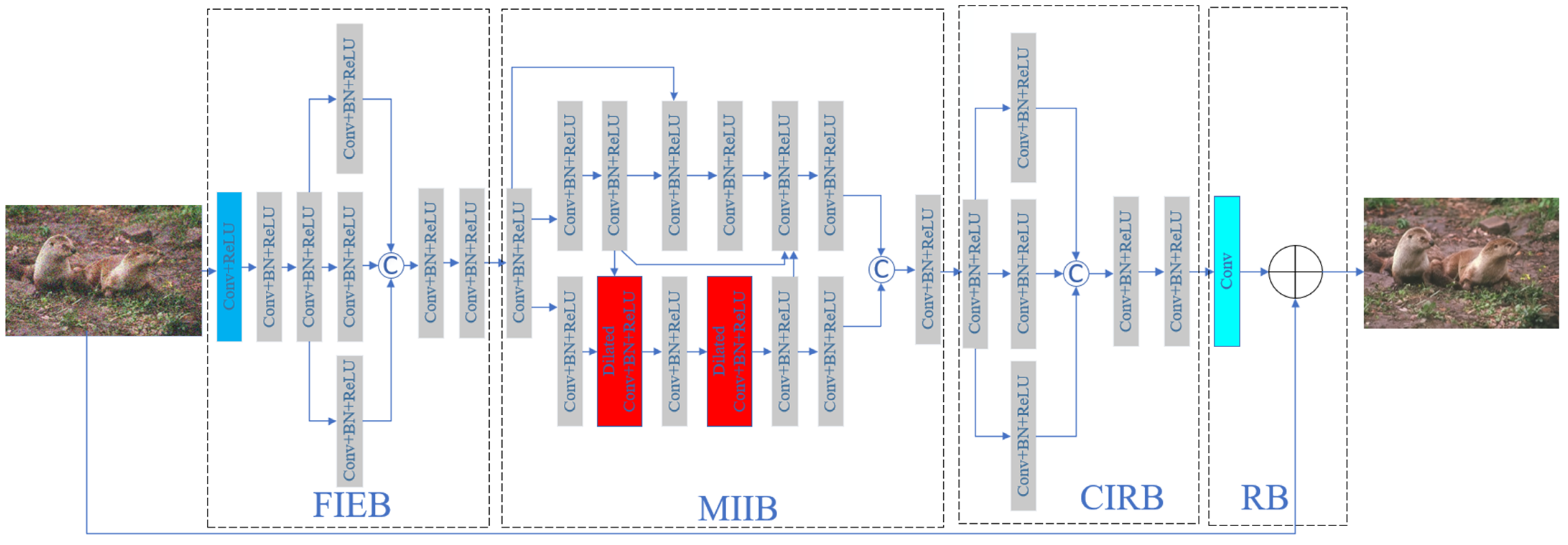
Therefore, in this paper we propose a multi-level information fusion CNN in image denoising (MLIFCNN). It consists of four blocks: a fine information extraction block (FIEB), a multi-level information interaction block (MIIB), a coarse information refinement block (CIRB), and a reconstruction block (RB). FIRB is in charge of extracting wide-channel information through parallel convolution groups. By using a two-layer interaction network, MIIB strengthens the fusion of wide and deep information, which is more conducive to obtaining more robust information. To enhance the stability of the training denoiser, CIRB stacks common and group convolutions to refine and obtain information. Finally, RB uses a residual operation to act in a single convolution to predict and obtain clean images. Our main contributions can be summarized as follows.
(1)
The proposed MLIFCNN incorporates multi-layer features and effectively improves the denoising performance;
(2)
FIEB utilizes different groups of odd convolutions to extract wide-channel information and enhance receptive fields to adapt to more complex image backgrounds;
(3)
MIIB uses dual-network interaction to strengthen the fusion of wide and deep information, which obtains more robust information when the noise level is unknown;
(4)
CIRB uses common and group convolutions to further enhance the stability of the trained denoiser.
The remainder of this paper is organized as follows. Section 2 provides related work of image denoising based on deep CNN, group convolution, and CNN-based feature fusion methods. Section 3 offers the proposed method. Section 4 shows experimental results. Section 5 presents the conclusion.

2. Related Work

This section is mainly responsible for introducing some of the related work involved in our paper, including some methods of CNN denoising, group convolution, and feature fusion from recent years. These three methods are described in detail below.

2.1. Image Denoising Based on Deep CNNs

Due to its strong learning capabilities, the CNN is often designed with various network architectures for handling relatively low-level visual tasks, such as image denoising [11]. For decades, most methods to improve denoising performance and efficiency have integrated new components into the CNN and, thus, improved network models. For example, Zhang et al. [21] combined a rectified linear unit (ReLU) [22], dilated convolution, and BN to improve the standard Res block, effectively improving the denoising performance. Gai et al. [23] integrated perceived loss, leakage flow linear unit (leakage ReLU), RL, and edge information into CNN to improve the performance of denoising. However, general CNN denoisers can easily lose detailed information in complex scenes, and, therefore, to recover precise details for complex tasks, Singh et al. [24] presented a new hybrid and multi-level digital image denoising method (MLAC) that combined anisotropic diffusion (AD) and CNN. In addition, different CNN models are able to solve different denoising problems. For example, to improve the practicability of the denoising algorithms, Anwar et al. [25] proposed a network with characteristic attention and residual structure to handle single-stage blind real images. In order to preserve the texture details of the image as much as possible while effectively denoising, Liu et al. [26] proposed a multiscale residual dense dual-attention network (MRDDANet). The method utilizes modules of different kernel sizes and dual-attention networks to extract features and combines global residuals to recover clean images. To balance the denoising time and the denoising performance, Zhang et al. [27] proposed a discrete shearlet transform (DST)-based denoising network (DSTnet). Furthermore, the combination of sparse-based low-rank representation method and CNN also has a good denoising effect on hyperspectral images [28]. CNN can also denoise medical images [29]. From the above method, we know that the deep CNN is very popular and effective in image denoising, and, inspired by this, our denoising network is also based on the basic CNN model.

2.2. Group Convolution

The appearance of group convolution [30] is very important for training very deep neural networks and can obtain better results with fewer parameters. Inspired by this, Tian et al. [31] divided feature maps into 1/4 channel and 3/4 channel groups and combined residual learning and group convolution to fully integrate deep and wide channel information to improve image super-resolution performance. Huang et al. [32] proposed a novel network architecture Condense-Net, which achieves efficient computing by combining dense connections with new modules called learning group convolution, where dense connectivity facilitates feature reuse in the network, while the learned group convolution removes the connections between the layers. Zhang et al. [33] proposed an interleaved group convolution consisting of primary group convolution and a secondary group. It utilizes the primary group convolution to deal with the spatial correlations, uses the secondary group convolution to mix the cross-partition channels of the primary group convolution output, and achieves good results in terms of accuracy and efficiency. Our denoising network also designs a new group convolution, which effectively improves the denoising performance.

2.3. CNN-Based Feature Fusion Methods

Feature fusion technologies have often been fused into the CNN to better improve efficiency and enhance performance. Therefore, many CNN-based feature interaction methods have been proposed in recent years, such as Guo et al. [34] who proposed a CNN-enhanced multi-level Haar wavelet feature fusion network (CNN-MHWF2N), which combines factor analysis, Harr wavelet decomposition, dual filtering, and fusion operators; effectively combines spatial and spectral information; and improves the classification performance of hyperspectral images. Tian et al. [35] proposed a dual denoising network (DudeNet), which extracted global and local features through a dual network with sparse mechanism and fused features using enhanced blocks to effectively recover image details. Zhao et al. [36] propose a pyramid denoising network, which uses the channel attention mechanism to recalibrate the channel importance, and then uses each branch of the pyramid structure to extract the global information and local information, and finally use multiple branches with different convolution kernel size for feature fusion, effectively solving the problem of blind denoising. Han et al. [37] propose a novel remote sensing image denoising network (RSIDNet), and this method effectively integrates the deep and shallow features of the image through multiple local jumps, retaining more image details. Inspired by this, the denoising networks mentioned in this paper also design a dual-network interaction block, which strengthens the fusion of wide information and deep information and obtains more robust information.

3. Method

In this subsection, we show our proposed denoising network model that consists of FIEB, MIIB, CIRB, and RB. For the design of the network architecture, we changed the form of the traditional grouping convolution [30] and integrated the residual connection and dilated convolution to better adapt to the image denoising. In order to improve the image denoising effect, we mainly removed the noise through the proposed three blocks of FIEB, MIIB, and CIRB. Specifically, FIEB uses the standard convolutions and parallel group convolutions to extract wide-channel information. To enhance the robustness of the obtained information, MIIB integrates the residual connection, dilated convolution, and standard convolution, and uses the form of dual-network interaction to fuse wide and deep information. To enhance the stability of the training denoiser, CIRB stacks common and group convolutions to refine obtain information.
Below, we properly describe the network model, network modules, and related functions we mentioned.

3.1. Network Model

The paper proposes a network model (MLIFCNN), which is made up of FIEB, MIIB, CIRB, and RB, as shown in Figure 1. To better clarify the expression process, we express it by the following formula:
I c = M L I F C N N ( I n ) = R B ( C I R B ( M I I B ( F I E B ( I n ) ) ) )
where I c expresses a predicted clean image, MLIFCNN denotes the function of MLIFCNN, and I n expresses a given noisy image. In addition, RB, CIRB, MIIB, and FIEB are also functions of RB, CIRB, MIIB, and FIEB, respectively.

3.2. Loss Function

In order to make our denoising network more persuasive, we selected mean square error (MSE) as the loss function to train the model parameters. This process can be described by the following formula:
L ( θ ) = 1 2 N i = 1 N M L I F C N N ( I n i ) I g t i 2
where I n i and I g t i denote the i-th noisy images and given clean images, respectively, and θ denotes the parameters in training the denoising model. In addition, N stands for the total of noisy images.

3.3. Peak Signal-to-Noise Ratio (PSNR)

In order to compare the experimental effect of image denoising more fairly, we chose the peak signal-to-noise ratio as our image quality evaluation technique, and its specific expression is as follows:
P S N R = 10 l o g 10 ( m a x v a l 2 ) / L ( θ )
where maxval represents the maximum value in the image data. If it is an 8-bit unsigned integer data type, maxval is 255. From Equation (3), we can see that it is a representation of absolute error in dB.

3.4. Fine Information Extraction Block

The fine information extraction block consists of standard and group convolution and is mainly used to extract wide-channel information. Specifically, the first layer is made up of a standard convolution and ReLU to extract the shallow features. Its kernel size is 3 × 3, and the input and output channels are 1 and 64, respectively. In extraordinary circumstances, if the network is used for denoising of color images, then its input channel is 3. The ReLU is responsible for converting linear features to non-linear features. The back five layers are an odd convolution group to extract the local wide-channel information and enhance the receptive fields. Specifically, the first two layers both consist of Conv + BN + ReLU, which stands for a combination of a convolutional layer, BN, and ReLU, respectively. The BN is an activation function. Their kernel sizes were 3 × 3, and the input and output channels are 64 and 32, respectively. This is to better preserve the global information for the next phase of training. They are then divided into three groups. The three groups are composed of Conv + BN + ReLU. Their kernel sizes are 3 × 3, 5 × 5, and 7 × 7, respectively. Input and output channels are 32. Finally, the three groups are combined into the latter two layers. The structures of the latter two and the first two layers are similar, except that both the input and output channels are increased to 32. To make the process clearer, we describe it using the following formula:
O F I E B = F I E B I n = C B R ( C B R ( C a t ( C B R C B R C B R C R I n , C B R 5 ( C B R ( C B R ( C R ( I n ) ) ) ) , C B R 7 ( C B R ( C B R ( C R ( I n ) ) ) ) ) ) )
where CR denotes 3 × 3 kernel size of Conv + ReLU, CBR stands for the 3 × 3 kernel size of Conv + BN + ReLU, CBR5 stands for the 5 × 3 kernel size of Conv + BN + ReLU, and CBR7 stands for the 7 × 7 kernel size of Conv + BN + ReLU. Cat represents the connection function C in Figure 1. O F I E B is the output of FIEB.

3.5. Multi-Level Information Interaction Block

The multi-level information interaction block integrates the skip connection, dilated convolution, and some standard convolutions, and uses the form of dual-network interaction to fuse wide and deep information, thus, making the obtained information more robust. The first layer is made up of Conv + BN + ReLU. Behind it is a block of dual-network interaction. The upper network consists of 6 layers, and every layer is made up of Conv + BN + ReLU. Their kernel size is 3 × 3. The lower network also consists of 6 layers, but the 1st, 3rd, 5th, and 6th layers are made up of Conv + BN + ReLU. The 2nd and 4th layers are made up of dilated convolution, BN, and ReLU. Then, the two-layer network input is connected to the last layer of this block. The last layer is also made up of a standard convolution, BN, and ReLU. The above description may be expressed as:
O M I I B = C B R ( C a t ( C B R ( C B R ( C a t ( C B R ( C B R ( C a t ( U 2 , C B R ( O F I E B ) ) ) ) , U 2 , L 5 ) ) ) , C B R ( L 5 ) ) ) L 5 = C B R ( D C B R 5 ( C B R ( D C B R 2 ( C a t ( C B R ( C B R ( O F I E B ) ) , U 2 ) ) ) ) ) U 2 = C B R ( C B R ( C B R ( O F I E B ) ) )
where DCBR2 represents the Conv + BN + ReLU of dilation = 2 and kernel size = 3 × 3, and DCBR5 represents the Conv + BN + ReLU of dilation = 5 and kernel size = 3 × 3. The O M I I B is the output of MIIB.

3.6. Coarse Information Refinement Block

The coarse information refinement block stacks common and group convolutions to refine obtained information. The first layer of the block is made up of Conv + BN + ReLU, and then it is output to three parallel group convolutions. To reduce the computational amount and expand the receptive field, we utilized the size convolution kernel. Thus, we set their kernels size separately to 1 × 1, 5 × 5, and 7 × 7. Finally, the 3 sets of outputs are connected to the last two-layer network of the block. For a clearer description, we express it by the following formula:
O C I R B = C B R ( C B R ( C a t ( C B R 1 C B R O M I I B , C B R 5 ( C B R ( O M I I B ) ) , C B R 7 ( C B R ( O M I I B ) ) ) ) )
where CBR1 denotes the 1 × 1 kernel size Conv + BN + ReLU. The O C I R B is the output of the CIRB.

3.7. Reconstruction Block

The reconstruction block uses a residual operation to act as a single convolution to predict and obtain clean images, and the process can be explained by the following formula:
I c = R B ( O C I R B ) = I n C ( O C I R B )
where C stand for the 3 × 3 kernel size convolution, − stands for a residual operation, as represented ⊕ in Figure 1.

4. Experiment

In this section, we present the datasets we selected and the settings of some experimental parameters, analyze and discuss ablation experiments and comparative experiments, and present the corresponding experimental data and denoising images.

4.1. Datasets

4.1.1. Training Datasets

We used different training sets for different types of images. For the grey synthetic noise images, we used 400 images with a size of 180 × 180 from the Berkeley Segmentation Dataset (BSD) [38] to train. For the color synthetic noise images, we used 432 color images with a size of 481 × 321 from BSD [38] for training. In addition, for further image feature description, we randomly divided gray training image into patches of size 40 × 40 and color training image into patches of size 50 × 50. For real noisy images, we used 100 real noisy images with a size of 512 × 512 from the benchmark dataset [39] to train the model. Also, to increase the diversity of the training sample, we enhanced the image by rotation of the image, such as rotating by 90° counterclockwise, horizontal flip, and rotating by 180° counterclockwise.

4.1.2. Test Datasets

To test the training effect of our model, we chose BSD68 [40] and Set12 [41] for the grey image test set, CBSD68 [40] for the color image test set, and CC [42] for the real image test set. Their number of images is 68, 12, 68, and 15, respectively.

4.2. Implementation Details

Among the parameters required by our model, the batch size is 128, the initial learning rate is 1 × 10⁻³, and the number of epochs is 120 and 70 for training the gray images and the color images, respectively. The learning rates vary from 1 × 10⁻³ to 1 × 10⁻⁵ with an increasing epoch. To accelerate the training speed, our experiments were all conducted on a GPU of Nvidia GeForce RTX 3090. Also, its CUDA was 11.7, and cuDNN was 8.0.4. Specifically, we used Pytorch 1.7.0, torchvision 0.8.1, and Python 3.8.13 to train and test our model MLIFCNN.

4.3. Network Analysis

The proposed denoising model (MLIFCNN) includes FIEB, MIIB, CIRB, and RB, and below we specifically describe their rationality and effectiveness.
FIEB: As mentioned in the above method, it is a module that extracts the wide-channel information and enhances receptive fields. Due to grouping convolution [30], it can achieve good results by reducing the number of model parameters; we propose a parallel group convolution in FIEB. We set three different odd kernel sizes convolutions, of 3, 5, and 7. The benefits of such a setup can be illustrated by Table 1 and Table 2 from the ablation experiment. In Table 1, we find MLIFCNN has a higher PSNR result than MLIFCNN without group convolutions in FIEB. From Table 2, we can see that the setting of this parameter has a higher PRNR value. Therefore, the proposed parallel group convolutions are effective in image denoising.
MIIB: It is a double-layer interaction module. In general, the interaction between different modules is conducive to the complementarity of global information and local information, increasing horizons and improving model learning ability [35]. Inspired by this, we used a six-layer Conv + BN + ReLU in the upper network and combined it with the jump connection to interact with the lower network. Also, we used two-layer dilated Conv + BN + ReLU and four-layer standard Conv + BN + ReLU in lower networks to obtain more contextual information. We can clearly see in Table 1 that MLIFCNN has higher PSNR values than MLIFCNN without residual connection and dilated convolution in MIIB. Therefore, the interaction network that we improve is beneficial to denoising.
CIRB: It is a module used to enhance the stability of the training denoiser. We used a group convolution similar to the FIEB module, except for the convolution kernel sizes of 1, 5, and 7 upon grouping. As can be seen in Table 1, MLIFCNN has a higher PSNR result than MLIFCNN without group convolutions in CIRB. From Table 2, we can see that the setting of this parameter has a higher PRNR value. This shows that the group convolutions do enhance the denoising performance.
RB: To output the clear image that we want to predict, we use a residual operation to act as a single convolution, with the effect shown in Figure 1.

4.4. Comparison with the State-of-the-Art Denoising Methods

In this section, in order to test denoising performance of MLIFCNN, we performed the analysis from both quantitative and qualitative perspectives. For the quantitative analysis, we compared the PSNR, running time, and complexity with many competitive denoising methods, such as: MLP [43], CNLNet [44], BM3D [45], enhanced convolutional neural denoising network (ECNDNet) [15], DnCNN [13], TNRD [46], FFDNet [47], a hybrid denoising CNN (HDCNN) [48], EPLL [49], image restoration CNN (IRCNN) [12], weighted nuclear norm minimization (WNNM) [50], attention-guided CNN (ADNet) [51], RDDCNN [52], cascade of shrinkage fields (CSF) [53], MemNet [54], residual encoder decoder network (RED30) [55], deep universal blind denoiser (DUBD) [56], contourlet-transform-based CNN (CTCNN) [57], adaptively tuned denoising network (ATDNet) [58], CBM3D [59], neat image (NI) [60], and TID [61]. We mainly denoise the synthetic noise images and real images. Synthetic noise images include gray and color synthetic noise images, and their noise levels include a specific value and vary from 0 to 55. Noise images with different noise levels are called blind noise images. Therefore, we performed the following comparative experiments.
To test the denoising performance of MLIFCNN on gray Gaussian synthetic noisy images, we compared PSNR with certain competitive methods on the datasets BSD68 and Set12. The experimental results are shown in Table 3 and Table 4. We can see from Table 3 and Figure 2 that our PSNR results are both the highest in the denoising levels of 15, 25, and 50. Similarly, we can see from Table 4 that the average PSNR values are the best at the denoising levels 15 and 25, and are also better at 50.
To test the denoising performance of MLIFCNN in color Gaussian synthetic noisy image, we compared PSNR with some better methods on the dataset CBSD68, and its experimental results are shown in Table 5. From Figure 3, we can see that our method has a very good PSNR results on the dataset CBSD68, and that it is optimal at the noise levels of 25 and 50. Second, from Table 5, we also find that the blind denoising PSNR value of our color images is better than the partial method under specific noise conditions. This shows that our method is very effective in color blind denoising.
Moreover, our proposed MLIFCNN is excellent on the real-world noisy image dataset CC. As shown in Table 6, our average PSNR value is 0.51 dB higher than ADNet and 2.34 dB higher than DnCNN. This shows that our denoising method performs well in real noisy images.
We can see from Table 7 that we selected 10 excellent methods for comparison to test the denoise run-time from noise images of different sizes (i.e., 256 × 256, 512 × 512, and 1024 × 1024). Compared to these methods, the running time is very short. Also, we tested the complexity of the model, as shown in Table 8. We find that the parameters of our model are still relatively few.
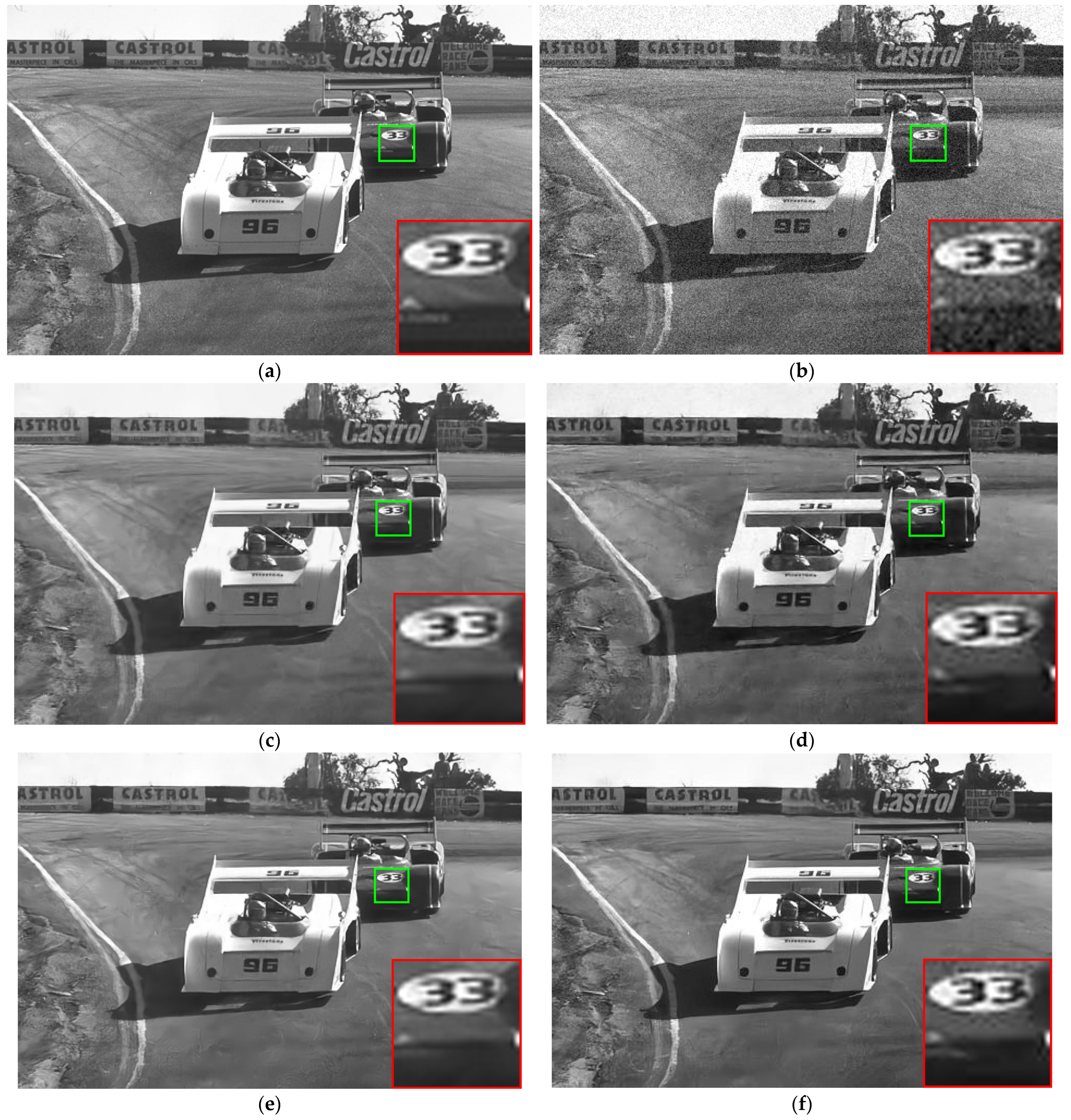
In terms of qualitative analysis, we apply some visual figures from BSD68, Set12, and CBSD68 to present the denoising effect of different methods. We can see the visual effect of the grey image being denoised from Figure 4 and Figure 5. Moreover, as shown in Figure 6, we can see the effect of the color image denoising. From these Figures, we choose a predictive image area to amplify as the observed area, and find that our method is clearer than some state-of-the-art denoising methods. In order to denoise the results more clearly in the table, we use red and blue lines to express the best and second-best PSNR values, respectively. According to the above experimental analysis, our denoising model is very efficient.

5. Conclusions

In this paper, we propose a multi-level information fusion CNN (MLIFCNN) for image denoising. MLIFCNN mainly denoises through three blocks: FIEB, MIIB, and CIRB. Specifically, FIEB uses parallel group convolution to extract wide-channel information and enhance receptive fields to adapt to more complex image backgrounds. The MIIB realizes the interaction of wide and deep information through two sub-networks, which better adapts it to the distribution of different noise levels and enhances the robustness of obtained information. The CIRB further enhances the stability of the training denoiser and improves the denoising performance by combining the size convolutional kernel and group convolution. After performing the above three blocks, RB uses a residual operation to act as a single convolution to predict and obtain clean images. Experimental results show that our proposed MLIFCNN is very effective in both quantitative and qualitative evaluation.
Although we show that the multi-level information fusion CNN method can indeed achieve image denoising well, we can also combine transformers or some heterogeneous network fusion methods in the future to further enhance the performance of real image denoising.

Author Contributions

Conceptualization, S.X., J.S., Y.H. and C.Z.; Methodology, S.Z. All authors have read and agreed to the published version of the manuscript.

Funding

This work was supported in part by Key Project of NSFC under grant 61836016 and Project of NSFC under grant 62072166.

Data Availability Statement

The selected dataset are all publicly available and easily available online. For specific code and data, please contact the corresponding author.

Conflicts of Interest

The authors declare no conflict of interest.

References

  1. Healey, G.E.; Kondepudy, R. Radiometric CCD camera calibration and noise estimation. IEEE Trans. Pattern Anal. Mach. Intell. 1994, 16, 267–276. [Google Scholar] [CrossRef]
  2. Fan, L.; Zhang, F.; Fan, H.; Zhang, C. Brief review of image denoising techniques. Vis. Comput. Ind. Biomed. Art 2019, 2, 1–12. [Google Scholar] [CrossRef] [PubMed]
  3. Gurrola-Ramos, J.; Dalmau, O.; Alarcón, T.E. A residual dense U-Net neural network for image denoising. IEEE Access 2021, 9, 31742–31754. [Google Scholar] [CrossRef]
  4. Li, H.; Suen, C.Y. A novel non-local means image denoising method based on grey theory. Pattern Recognit. 2016, 49, 237–248. [Google Scholar] [CrossRef]
  5. Zhang, J.; Cao, L.; Wang, T.; Fu, W.; Shen, W. NHNet: A non-local hierarchical network for image denoising. IET Image Process. 2022, 16, 2446–2456. [Google Scholar] [CrossRef]
  6. Xiao, J.; Zhao, R.; Lam, K.M. Bayesian sparse hierarchical model for image denoising. Signal Process. Image Commun. 2021, 96, 116299. [Google Scholar] [CrossRef]
  7. Shi, M.; Zhang, F.; Wang, S.; Zhang, C.; Li, X. Detail preserving image denoising with patch-based structure similarity via sparse representation and SVD. Comput. Vis. Image Underst. 2021, 206, 103173. [Google Scholar] [CrossRef]
  8. Zhou, T.; Li, C.; Zeng, X.; Zhao, Y. Sparse representation with enhanced nonlocal self-similarity for image denoising. Mach. Vis. Appl. 2021, 32, 110. [Google Scholar] [CrossRef]
  9. Guo, S.; Wang, G.; Han, L.; Song, X.; Yang, W. COVID-19 CT image denoising algorithm based on adaptive threshold and optimized weighted median filter. Biomed. Signal Process. Control. 2022, 75, 103552. [Google Scholar] [CrossRef]
  10. Pang, Z.-F.; Zhou, Y.-M.; Wu, T.; Li, D.-J. Image denoising via a new anisotropic total-variation-based model. Signal Process. Image Commun. 2019, 74, 140–152. [Google Scholar] [CrossRef]
  11. Tian, C.; Fei, L.; Zheng, W.; Xu, Y.; Zuo, W.; Lin, C.-W. Deep learning on image denoising: An overview. Neural Netw. 2020, 131, 251–275. [Google Scholar] [CrossRef]
  12. Zhang, K.; Zuo, W.; Gu, S.; Zhang, L. Learning deep CNN denoiser prior for image restoration. In Proceedings of the IEEE Conference on Computer Vision and Pattern Recognition, Honolulu, HI, USA, 26 July 2017; pp. 3929–3938. [Google Scholar]
  13. Zhang, K.; Zuo, W.; Chen, Y.; Meng, D.; Zhang, L. Beyond a gaussian denoiser: Residual learning of deep cnn for image denoising. IEEE Trans. Image Process. 2017, 26, 3142–3155. [Google Scholar] [CrossRef] [PubMed]
  14. Quan, Y.; Chen, Y.; Shao, Y.; Teng, H.; Xu, Y.; Ji, H. Image denoising using complex-valued deep CNN. Pattern Recognit. 2021, 111, 107639. [Google Scholar] [CrossRef]
  15. Tian, C.; Xu, Y.; Fei, L.; Wang, J.; Wen, J.; Luo, N. Enhanced CNN for image denoising. CAAI Trans. Intell. Technol. 2019, 4, 17–23. [Google Scholar] [CrossRef]
  16. He, K.; Zhang, X.; Ren, S.; Sun, J. Deep residual learning for image recognition. In Proceedings of the IEEE Conference on Computer Vision and Pattern Recognition, Las Vegas, NV, USA, 27–30 June 2016; pp. 770–778. [Google Scholar]
  17. Ioffe, S.; Szegedy, C. Batch normalization: Accelerating deep network training by reducing internal covariate shift. In Proceedings of the International Conference on Machine Learning, Lille, France, 11 July 2015; pp. 448–456. [Google Scholar]
  18. Zhao, M.; Cao, G.; Huang, X.; Yang, L. Hybrid Transformer-CNN for Real Image Denoising. IEEE Signal Process. Lett. 2022, 29, 1252–1256. [Google Scholar] [CrossRef]
  19. Kumwilaisak, W.; Piriyatharawet, T.; Lasang, P.; Thatphithakkul, N. Image denoising with deep convolutional neural and multi-directional long short-term memory networks under Poisson noise environments. IEEE Access 2020, 8, 86998–87010. [Google Scholar] [CrossRef]
  20. Pang, T.; Zheng, H.; Quan, Y.; Ji, H. Recorrupted-to-recorrupted: Unsupervised deep learning for image denoising. In Proceedings of the IEEE/CVF Conference on Computer Vision and Pattern Recognition, Nashville, TN, USA, 20–25 June 2021; pp. 2043–2052. [Google Scholar]
  21. Zhang, J.; Zhu, Y.; Li, W.; Fu, W.; Cao, L. DRNet: A deep neural network with multi-layer residual blocks improves image denoising. IEEE Access 2021, 9, 79936–79946. [Google Scholar] [CrossRef]
  22. Glorot, X.; Bordes, A.; Bengio, Y. Deep sparse rectifier neural networks. In Proceedings of the Fourteenth International Conference on Artificial Intelligence and Statistics, Fort Lauderdale, FL, USA, 11–13 April 2011; JMLR Workshop and Conference Proceedings. pp. 315–323. [Google Scholar]
  23. Gai, S.; Bao, Z. New image denoising algorithm via improved deep convolutional neural network with perceptive loss. Expert Syst. Appl. 2019, 138, 112815. [Google Scholar] [CrossRef]
  24. Singh, P.; Shankar, A. A novel optical image denoising technique using convolutional neural network and anisotropic diffusion for real-time surveillance applications. J. Real-Time Image Process. 2021, 18, 1711–1728. [Google Scholar] [CrossRef]
  25. Anwar, S.; Barnes, N. Real image denoising with feature attention. In Proceedings of the IEEE/CVF International Conference on Computer Vision, Seoul, Republic of Korea, 27 October–2 November 2019; pp. 3155–3164. [Google Scholar]
  26. Liu, S.; Lei, Y.; Zhang, L.; Li, B.; Hu, W.; Zhang, Y.-D. MRDDANet: A multiscale residual dense dual attention network for SAR image denoising. IEEE Trans. Geosci. Remote Sens. 2021, 60, 1–13. [Google Scholar] [CrossRef]
  27. Lyu, Z.; Zhang, C.; Han, M. DSTnet: A new discrete shearlet transform-based CNN model for image denoising. Multimed. Syst. 2021, 27, 1165–1177. [Google Scholar] [CrossRef]
  28. Sun, H.; Liu, M.; Zheng, K.; Yang, D.; Li, J.; Gao, L. Hyperspectral image denoising via low-rank representation and CNN denoiser. IEEE J. Sel. Top. Appl. Earth Obs. Remote Sens. 2021, 15, 716–728. [Google Scholar] [CrossRef]
  29. Rawat, S.; Rana, K.P.S.; Kumar, V. A novel complex-valued convolutional neural network for medical image denoising. Biomed. Signal Process. Control. 2021, 69, 102859. [Google Scholar] [CrossRef]
  30. Krizhevsky, A.; Sutskever, I.; Hinton, G.E. Imagenet classification with deep convolutional neural networks. Adv. Neural Inf. Process. Syst. 2012, 25, 84–90. [Google Scholar] [CrossRef]
  31. Tian, C.; Yuan, Y.; Zhang, S.; Lin, C.-W.; Zuo, W.; Zhang, D. Image Super-resolution with An Enhanced Group Convolutional Neural Network. arXiv 2022, arXiv:2205.14548. [Google Scholar]
  32. Huang, G.; Liu, S.; Van der Maaten, L.; Weinberger, K.Q. Condensenet: An efficient densenet using learned group convolutions. In Proceedings of the IEEE Conference on Computer Vision and Pattern Recognition, Salt Lake City, UT, USA, 18–23 June 2018; pp. 2752–2761. [Google Scholar]
  33. Zhang, T.; Qi, G.J.; Xiao, B.; Wang, J. Interleaved group convolutions. In Proceedings of the IEEE International Conference on Computer Vision, Venice, Italy, 22–29 October 2017; pp. 4373–4382. [Google Scholar]
  34. Guo, W.; Xu, G.; Liu, B.; Wang, Y. Hyperspectral Image Classification Using CNN-Enhanced Multi-Level Haar Wavelet Features Fusion Network. IEEE Geosci. Remote Sens. Lett. 2022, 19, 1–5. [Google Scholar] [CrossRef]
  35. Tian, C.; Xu, Y.; Zuo, W.; Du, B.; Lin, C.-W.; Zhang, D. Designing and training of a dual CNN for image denoising. Knowl.-Based Syst. 2021, 226, 106949. [Google Scholar] [CrossRef]
  36. Zhao, Y.; Jiang, Z.; Men, A.; Ju, G. Pyramid real image denoising network. In Proceedings of the 2019 IEEE Visual Communications and Image Processing (VCIP), Sydney, Australia, 1–4 December 2019; pp. 1–4. [Google Scholar]
  37. Han, L.; Zhao, Y.; Lv, H.; Zhang, Y.; Liu, H.; Bi, G. Remote Sensing Image Denoising Based on Deep and Shallow Feature Fusion and Attention Mechanism. Remote Sens. 2022, 14, 1243. [Google Scholar] [CrossRef]
  38. Martin, D.R.; Fowlkes, C.; Tal, D.; Malik, J. A database of human segmented natural images and its application to evaluating segmentation algorithms and measuring ecological statistics. In Proceedings of the Eighth IEEE International Conference on Computer Vision, Vancouver, BC, Canada, 7–14 July 2001; Volume 2, pp. 416–423. [Google Scholar]
  39. Xu, J.; Li, H.; Liang, Z.; Zhang, D.; Zhang, L. Real-world noisy image denoising: A new benchmark. arXiv 2018, arXiv:1804.02603. [Google Scholar]
  40. Roth, S.; Black, M.J. Fields of experts: A framework for learning image priors. In Proceedings of the 2005 IEEE Computer Society Conference on Computer Vision and Pattern Recognition (CVPR’05), San Diego, CA, USA, 20–26 June 2005; Volume 2, pp. 860–867. [Google Scholar]
  41. Mairal, J.; Bach, F.; Ponce, J.; Sapiro, G.; Zisserman, A. Non-local sparse models for image restoration. In Proceedings of the 2009 IEEE 12th International Conference on Computer Vision, Kyoto, Japan, 27 September–4 October 2009; pp. 2272–2279. [Google Scholar]
  42. Nam, S.; Hwang, Y.; Matsushita, Y.; Kim, S.J. A holistic approach to cross-channel image noise modeling and its application to image denoising. In Proceedings of the IEEE Conference on Computer Vision and Pattern Recognition, Las Vegas, NV, USA, 27–30 June 2016; pp. 1683–1691. [Google Scholar]
  43. Burger, H.C.; Schuler, C.J.; Harmeling, S. Image denoising: Can plain neural networks compete with BM3D? In Proceedings of the 2012 IEEE Conference on Computer Vision and Pattern Recognition, Providence, RI, USA, 16–21 June 2012; pp. 2392–2399. [Google Scholar]
  44. Lefkimmiatis, S. Non-local color image denoising with convolutional neural networks. In Proceedings of the IEEE Conference on Computer Vision and Pattern Recognition, Honolulu, HI, USA, 21–26 July 2017; pp. 3587–3596. [Google Scholar]
  45. Dabov, K.; Foi, A.; Egiazarian, K. Video denoising by sparse 3D transform-domain collaborative filtering. In Proceedings of the 2007 15th European Signal Processing Conference, Poznan, Poland, 3–7 September 2007; pp. 145–149. [Google Scholar]
  46. Chen, Y.; Pock, T. Trainable nonlinear reaction diffusion: A flexible framework for fast and effective image restoration. IEEE Trans. Pattern Anal. Mach. Intell. 2016, 39, 1256–1272. [Google Scholar] [CrossRef]
  47. Zhang, K.; Zuo, W.; Zhang, L. FFDNet: Toward a fast and flexible solution for CNN-based image denoising. IEEE Trans. Image Process. 2018, 27, 4608–4622. [Google Scholar] [CrossRef]
  48. Zheng, M.; Zhi, K.; Zeng, J.; Tian, C.; You, L. A Hybrid CNN for Image Denoising. J. Artif. Intell. Technol. 2022, 2, 93–99. [Google Scholar] [CrossRef]
  49. Zoran, D.; Weiss, Y. From learning models of natural image patches to whole image restoration. In Proceedings of the 2011 International Conference on Computer Vision, Barcelona, Spain, 6–13 November 2011; pp. 479–486. [Google Scholar]
  50. Gu, S.; Zhang, L.; Zuo, W.; Feng, X. Weighted nuclear norm minimization with application to image denoising. In Proceedings of the IEEE Conference on Computer Vision and Pattern Recognition, Columbus, OH, USA, 23–28 June 2014; pp. 2862–2869. [Google Scholar]
  51. Tian, C.; Xu, Y.; Li, Z.; Zuo, W.; Fei, L.; Liu, H. Attention-guided CNN for image denoising. Neural Netw. 2020, 124, 117–129. [Google Scholar] [CrossRef] [PubMed]
  52. Zhang, Q.; Xiao, J.; Tian, C.; Lin, J.C.-W.; Zhang, S. A robust deformed convolutional neural network (CNN) for image denoising. In CAAI Transactions on Intelligence Technology; Wiley Online Library: Hoboken, NJ, USA, 2022. [Google Scholar]
  53. Schmidt, U.; Roth, S. Shrinkage fields for effective image restoration. In Proceedings of the IEEE Conference on Computer Vision and Pattern Recognition, Columbus, OH, USA, 23–28 June 2014; pp. 2774–2781. [Google Scholar]
  54. Tai, Y.; Yang, J.; Liu, X.; Xu, C. Memnet: A persistent memory network for image restoration. In Proceedings of the IEEE International Conference on Computer Vision, Venice, Italy, 22–29 October 2017; pp. 4539–4547. [Google Scholar]
  55. Mao, X.; Shen, C.; Yang, Y.B. Image restoration using very deep convolutional encoder-decoder networks with symmetric skip connections. Adv. Neural Inf. Process. Syst. 2016, 29. [Google Scholar]
  56. Soh, J.W.; Cho, N.I. Deep universal blind image denoising. In Proceedings of the 2020 25th International Conference on Pattern Recognition (ICPR), Milan, Italy, 10–15 January 2021; pp. 747–754. [Google Scholar]
  57. Lyu, Z.; Zhang, C.; Han, M. A nonsubsampled countourlet transform based CNN for real image denoising. Signal Process. Image Commun. 2020, 82, 115727. [Google Scholar] [CrossRef]
  58. Kim, Y.; Soh, J.W.; Cho, N.I. Adaptively tuning a convolutional neural network by gate process for image denoising. IEEE Access 2019, 7, 63447–63456. [Google Scholar] [CrossRef]
  59. Dabov, K.; Foi, A.; Katkovnik, V.; Egiazarian, K. Color image denoising via sparse 3D collaborative filtering with grouping constraint in luminance-chrominance space. In Proceedings of the 2007 IEEE International Conference on Image Processing, San Antonio, TX, USA, 16–19 September 2007; Volume 1, pp. I-313–I-316. [Google Scholar]
  60. ABSoft, NeatLab. Neat Image. 2017. Available online: https://ni.neatvideo.com/ (accessed on 20 March 2023).
  61. Luo, E.; Chan, S.H.; Nguyen, T.Q. Adaptive image denoising by targeted databases. IEEE Trans. Image Process. 2015, 24, 2167–2181. [Google Scholar] [CrossRef]
Figure 1. Network model of the proposed MLIFCNN.
Electronics 12 02146 g001
Figure 2. PSNR (dB) values of different denoising methods on gray test dataset BSD68 with noise level of 15, 25, and 50.
Electronics 12 02146 g002
Figure 3. PSNR (dB) values of different denoising methods on color test dataset CBSD68 with noise levels of 15, 25, and 50.
Electronics 12 02146 g003
Figure 4. PSNR values of different denoising methods on one image from BSD68 when noise level is 15. (a) Original image; (b) noisy image/24.62 dB; (c) FFDNet [47]/30.38 dB; (d) BM3D [45]/30.95; (e) IRCNN [12]/31.49 dB; (f) DnCNN [13]/31.74 dB; (g) ADNet [51]/31.76; (h) MLIFCNN/31.81 dB.
Electronics 12 02146 g004aElectronics 12 02146 g004b
Figure 5. PSNR values of different denoising methods on one image from Set12 when noise level is 50. (a) Original image; (b) noisy image/13.66 dB; (c) FFDNet [47]/25.89 dB; (d) BM3D [45]/25.10 dB; (e) IRCNN [12]/25.89 dB; (f) DnCNN [13]/25.87 dB; (g) RDDCNN [52]/25.88 dB; (h) MLIFCNN/25.92 dB.
Electronics 12 02146 g005aElectronics 12 02146 g005b
Figure 6. PSNR values of different denoising methods on one image from CBSD68 when noise level is 25. (a) Original image; (b) noisy image/16.68 dB; (c) IRCNN [12]/28.50 dB; (d) DnCNN [13]/28.81 dB; (e) ADNet [51]/28.56 dB; (f) MLIFCNN/28.86 dB.
Electronics 12 02146 g006aElectronics 12 02146 g006b
Table 1. PSNR (dB) values of different denoising methods on gray test dataset BSD68 with noise level of 15.
MethodsPSNR (dB)
MLIFCNN without group convolutions in FIEB31.745
MLIFCNN without group convolutions, dilated convolution, residual connections in FIEB and MIIB31.717
MLIFCNN without group convolutions, dilated convolution, residual connections in MIIB and CIRB31.418
MLIFCNN without dilated convolution, residual connections in MIIB31.726
MLIFCNN without group convolutions in CIRB31.756
MLIFCNN31.798
Table 2. PSNR (dB) values of different group convolution kernel methods on gray test dataset BSD68 with noise level of 15. In order to denoise the results more clearly in the table, we use red and blue lines to express the best and second-best PSNR values, respectively.
Methods FIEB CIRB PSNR (dB)
1, 3, 51, 5, 73, 5, 71, 3, 51, 5, 73, 5, 7
MLIFCNN 31.68
31.71
31.73
31.74
31.72
31.74
31.76
31.80
31.77
Table 3. PSNR (dB) values of different denoising methods on gray test dataset BSD68 with noise level of 15, 25, and 50.
MethodsBM3D [45]ECNDNet [15]DnCNN [13]TNRD [46]HDCNN [48]FFDNet [47]
σ = 1531.0731.7131.7231.4231.7431.63
σ = 2528.5729.2229.2328.9229.2529.19
σ = 5025.6226.2326.2325.9726.2326.29
EPLL [49]IRCNN [12]WNNM [50]ADNet [51]RDDCNN [52]MLIFCNNMLCNN-B
31.2131.6331.3731.7431.7631.8031.46
28.6829.1528.8329.2529.2729.2929.08
25.6726.1925.8726.2926.3026.3226.28
Table 4. Average PSNR (dB) values of different denoising methods on gray test dataset Set12 with noise levels of 15, 25, and 50.
ImagesC.manHousePeppersStarfishMonarchAirplaneParrotLenaBarbaraBoatManCoupleAverage
Noise level15
DnCNN [12]32.6134.9733.332.233.0931.731.8334.6232.6432.4232.4632.4732.86
ECNDNet [15]32.5634.9733.2532.1733.1131.731.8234.5232.4132.3732.3932.3932.81
RDDCNN [52]32.6135.0133.3132.1333.1331.6731.9334.5732.6232.4232.3832.4632.85
IRCNN [13]32.5534.8933.3132.0232.8231.731.8434.5332.4332.3432.432.432.77
FFDNet [47]32.4335.0733.2531.9932.6631.5731.8134.6232.5432.3832.4132.4632.77
WNNM [50]32.1735.1332.9931.8232.7131.3931.6234.2733.632.2732.1132.1732.7
EPLL [49]31.8534.1732.6431.1332.131.1931.4233.9231.3831.933231.9332.14
BM3D [45]31.9134.9332.6931.1431.8531.0731.3734.2633.132.1331.9232.132.37
TNRD [46]32.1934.5333.0431.7532.5631.4631.6334.2432.1332.1432.2332.1132.5
MLIFCNN32.6235.0633.3332.2633.2131.6931.9734.632.6332.2832.332.4532.87
MLIFCNN-B32.2834.8533.1231.9532.8931.4731.7834.3532.1132.2432.1232.2532.62
Noise level25
DnCNN [13]30.1833.0630.8729.4130.2829.1329.4332.443030.2130.130.1230.43
ECNDNet [15]30.1133.0830.8529.4330.329.0729.3832.3829.8430.1430.0330.0330.39
RDDCNN [52]30.233.1330.8229.3830.3629.0529.5332.430.0330.1930.0530.130.44
IRCNN [12]30.0833.0630.8829.2730.0929.1229.4732.4329.9230.1730.0430.0830.38
FFDNet [47]30.133.2830.9329.3230.0829.0429.4432.5730.0130.2530.1130.230.44
WNNM [50]29.6433.2230.4229.0329.8428.6929.1532.2431.2430.0329.7629.8230.26
EPLL [49]29.2632.1730.1728.5129.3929.6128.9531.7328.6129.7429.6629.5329.69
BM3D [45]29.4532.8530.1628.5629.2528.4228.9332.0730.7129.929.6129.7129.97
TNRD [46]29.7232.5330.5729.0230.8528.8829.183229.4129.9129.8729.7130.06
MLIFCNN30.2233.1630.7829.4530.3629.0829.532.4630.0730.2130.0630.1530.46
MLIFCNN-B29.9733.0230.729.2430.2128.9129.4232.2129.5129.9929.8329.9130.25
Noise level50
DnCNN [13]27.033027.3225.726.7825.8726.4829.3926.2227.227.2426.927.18
ECNDNet [15]27.0730.1227.325.7226.8225.7926.3229.2926.2627.1627.1126.8427.15
RDDCNN [52]27.1630.2127.3825.7226.8425.8826.5329.3226.3627.2327.2226.8827.23
IRCNN [12]26.8829.9627.3325.5726.6125.8926.5529.426.2427.1727.1726.8827.14
FFDNet [47]27.0530.3727.5425.7526.8125.8926.5729.6626.4527.1327.2927.0827.32
WNNM [50]26.4530.3326.9525.4426.3225.4226.1429.2527.7926.9726.9426.6427.05
EPLL [49]26.129.1226.825.1225.9425.3125.9528.6824.8326.7426.7926.326.47
BM3D [45]26.1329.6926.6825.0425.8225.125.929.0527.2226.7826.8126.4626.72
TNRD [46]26.6229.4827.125.4226.3125.5926.1628.9325.726.9426.9826.526.81
MLIFCNN27.230.3827.3925.7526.8925.9226.5729.4326.5327.2827.2627.0227.3
MLIFCNN-B27.0830.227.2925.6426.825.8526.4729.326.2727.227.1826.8727.18
Table 5. PSNR (dB) values of different denoising methods on color test dataset CBSD68 with noise levels of 15, 25, and 50.
DatasetsMethodsσ = 15σ = 25σ = 50
FFDNet [47]33.8031.1827.96
MLP [43]32.0728.9226.00
TNRD [46]31.3726.8825.94
CNLNet [44]33.8731.2127.96
CBSD68CBM3D [59]33.5230.7127.38
DnCNN [13]33.9831.3128.01
IRCNN [12]33.8631.1627.86
ADNet [51]33.9931.3128.04
MLIFCNN33.9531.3128.07
MLIFCNN-B33.9731.3128.04
Table 6. Average PSNR (dB) values of different denoising methods on real-world dataset CC.
Camera SettingsCBM3D [59]DnCNN [13]NI [60]ADNet [51]CSF [53]TID [61]MLIFCNN
Cannon 5 D ISO = 3200_139.7637.2637.6835.9635.6837.2237.65
Cannon 5 D ISO = 3200_236.434.1334.8736.1134.0334.5436.58
Cannon 5 D ISO = 3200_336.3734.0934.7734.4932.6334.2535.95
Nikon D600 ISO = 3200_134.1833.6234.1233.9431.7832.9935.05
Nikon D600 ISO = 3200_235.0734.4835.3634.3335.1632.9935.6
Nikon D600 ISO = 3200_337.1335.4138.6838.8739.9835.5838.25
Nikon D800 ISO = 1600_136.8137.9537.3437.6134.8434.4938.41
Nikon D800 ISO = 1600_237.7636.0838.5738.2438.4234.4939.14
Nikon D800 ISO = 1600_337.5135.4837.8736.8935.7935.2637.91
Nikon D800 ISO = 3200_135.0534.0836.9537.238.3633.737.02
Nikon D800 ISO = 3200_234.0733.735.0935.6735.5331.0436.24
Nikon D800 ISO = 3200_334.4233.3136.9138.0940.0533.0736.75
Nikon D800 ISO = 6400_131.1329.8331.2832.2434.0829.432.9
Nikon D800 ISO = 6400_231.2230.5531.3832.5932.1329.432.58
Nikon D800 ISO = 6400_330.9730.0931.433.1431.5229.2132.94
Average35.1933.8635.4935.6935.3333.3636.2
Table 7. Running time of different denoising methods for the noisy images of sizes 256 × 256, 512 × 512, and 1024 × 1024.
MethodsDevice256 × 256512 × 5121024 × 1024
WNNM [50]CPU203.1773.22536.4
CSF [43]CPU0.921.72
TNRD [46]CPU0.451.334.61
BM3D [45]CPU0.592.5210.77
MemNet [54]GPU0.87753.60614.69
ADNet [51]GPU0.04670.07980.2077
CTCNN [57]GPU0.0680.1030.364
RED30 [55]GPU1.3624.70215.77
DnCNN [13]GPU0.03440.06810.1556
MLIFCNNGPU0.01880.06780.2075
Table 8. Complexity of different denoising methods.
MethodsParametersFlops
DnCNN [13]0.56 M0.891 G
ADNet [51]0.52 M0.832 G
DUBD [56]2.09 M-
RED30 [55]4.13 M10.33 G
ATDNet [58]9.45 M-
MLIFCNN0.66 M1.49 G
Disclaimer/Publisher’s Note: The statements, opinions and data contained in all publications are solely those of the individual author(s) and contributor(s) and not of MDPI and/or the editor(s). MDPI and/or the editor(s) disclaim responsibility for any injury to people or property resulting from any ideas, methods, instructions or products referred to in the content.

