Color and Texture Analysis of Textiles Using Image Acquisition and Spectral Analysis in Calibrated Sphere Imaging System-II

Abstract

The extended application of device-dependent systems’ vision is growing exponentially, but these systems face challenges in precisely imitating the human perception models established by the device-independent systems of the Commission internationale de l’éclairage (CIE). We previously discussed the theoretical treatment and experimental validation of developing a calibrated integrated sphere imaging system to imitate the visible spectroscopy environment. The RGB polynomial function was derived to obtain a meaningful interpretation of color features. In this study, we dyed three different types of textured materials in the same bath with a yellow reactive dye at incremental concentrations to see how their color difference profiles tested. Three typical cotton textures were dyed with three ultra-RGB remozol reactive dyes and their combinations. The color concentration ranges of 1%, 2%, 3%, and 4% were chosen for each dye, followed by their binary and ternary mixtures. The aim was to verify the fundamental spectral feature mapping in various imaging color spaces and spectral domains. The findings are quite interesting and help us to understand the ground truth behind working in two domains. In addition, the trends of color mixing, CIE color difference, CIExy (chromaticity) color gamut, and RGB gamut and their distinguishing features were verified. Human perception accuracy was also compared in both domains to clarify the influence of texture. These fundamental experiments and observations on human perception and calibrated imaging color space could clarify the expected precision in both domains.

1. Introduction

We discussed the significance of this study, prior art, and theoretical treatment of imaging from an integrating sphere in our previous paper [1]. We experimented with textile texture and color by varying these factors in a controlled manner (red, blue, yellow, and cyan dyes at various concentrations (0.25%, 0.5%, 0.75%, 1%, 1.5%, 2%, 3%, 4%, 5%, and 6%)). In addition, a simple calibration technique that describes how unique digital color signatures can be derived from calibrated RGB to extract the best features for color and texture was proposed and validated. This alter ego of the reflectance function, missing in the imaging domain, was experimentally validated to be used for visualization, identification, and application for qualitative and quantitative color–texture analysis [1].

The present investigation aims to conduct a qualitative and quantitative analysis of color perception in terms of DERGB and DE precision using our proposed method, along with a study of color combination. Further, we studied various RGB spaces that were critically represented with varied texture and color combinations.

Many applications such as spectral measurements, image processing, and human vision require congruent and precise results in real-world problems. Complex operations, such as calibration protocols, device profiling, illumination uniformity, viewing geometry, device characterization, and so on, are used to bridge the gap between device-dependent and device-independent color transformation. In most cases, the characterization or prediction models are prone to theoretical assumption errors [1,2,3] as well as practical imperfections or limitations [4,5]. It could be stated that the illumination source’s properties and its uniformity over the material are likely the main offenders and play a crucial role in the precise estimation of color and texture qualities [6,7].

Most of the challenges were discussed in our previous article, and it is noteworthy here to mention some conclusive inferences from a few current researchers. Nie et al. (2023) [8] reported on problems with serious interference of specular reflections in the endoscopic image that majorly contribute to errors in computer vision algorithms. Abdulateef and Hasoon (2023) [9] studied the limitations of image analysis as it essentially needs a clear, bright, and no-shadow RGB image to obtain accurate results. As stated by Lin and Finlayson (2023) [10], “Surprisingly, we show that all compared algorithms—regardless of their model complexity—degrade to broadly the same level of performance.”

As a matter of fact, the device-dependent systems of RGB color spaces were knowingly evolved with the color compressed gamut of CIE and encouraged widely as a tool for easy communication, real-time application, business, and so on, with the growth of users of computers, phones, and other digital media [1,3]. As of today, it is a big challenge for AI systems and advanced algorithms to be trained accurately with prior domain knowledge for better identification, classification, and prediction of subjects or materials of interest. Nature has many colors and it may be beyond our knowledge how they react physically for our color perception. In physics terms, reflection, transmission, absorption, and scattering within the visible range of light involve numerous materials like dyes, pigments, and biomaterials for varied applications.

Materials show their unique properties of light reflectance and absorption over the visible range. If a substrate is dyed, we can see its family of curves by increasing the dye concentration (e.g., Figure 1). Interestingly, textile materials are quite suitable for experimenting with varied textures and dyes.

We dyed three different types of textured materials with a yellow reactive dye at incremental concentrations in the same bath. Dyeing experiments for three ultra-RGB remozol reactive dyes and their combinations were then carried out on the same substrate for four concentration ranges (single, binary, and ternary mixtures) to validate the fundamental spectral feature mapping in both domains and varied imaging color spaces. The motivation behind these ground truth experiments was to analyze the critical issue of human perception and computer vision: the device-independent human perception CIE model and current progress in digital image processing, with a simplified explanation.

2. Materials and Methods

In our previous study, we discussed the development of a novel integrating sphere imaging system with a theoretical explanation. We experimented with textile properties by varying the texture in a controlled way and coloring the samples with red, blue, yellow, and cyan dyes at various concentrations (0.25%, 0.5%, 0.75%, 1%, 1.5%, 2%, 3%, 4%, 5%, and 6%). We experimented and derived calibrated RGB polynomials and compared them with spectral measurement profiles. Procedures to precisely define the qualitative and quantitative influences of color and texture and color prediction capabilities were also planned and investigated. The present investigation aims to conduct a qualitative and quantitative analysis of the precision of our proposed method along with an analysis of color combination. Three types of bleached cotton fabrics with plain, twill, and modified twill were initially dyed in the same dye bath with a yellow reactive dye (Levafix Brilliant Yellow 4GL; vinyl sulphone class) in an incremental order of concentration, i.e., 0.25%, 0.5%, 0.75%, 1%, 1.5%, 2%, 2.5%, 3%, 4%, and 5% (10 shades for each of the three textures). Further, dyeing was carried out with three kinds of ultra-RGB Remozol reactive dyes and their combinations (single, binary, and ternary mixtures) on the same substrate in four concentration ranges: 1%, 2%, 3%, and 4% (Ultra-RGB Carmen (Dye A), Navy Blue (Dye B), and Red (Dye C)). The dyes were provided by Dystar, Hong Kong. A Minolta 2600D spectrophotometer was used to measure reflectance (360 to 740 nm with a 10 nm gap), XYZ, CIEL*a*b*, and color difference (DE). Images of plain, twill, and modified twill samples of the same percentage shade were taken together (Figure 2) and, after calibrating the diffused imaging system with a white tile, their average RGB values were computed in MATLAB. All the detailed measurement values are provided as Supplementary File.

3. Results and Discussion

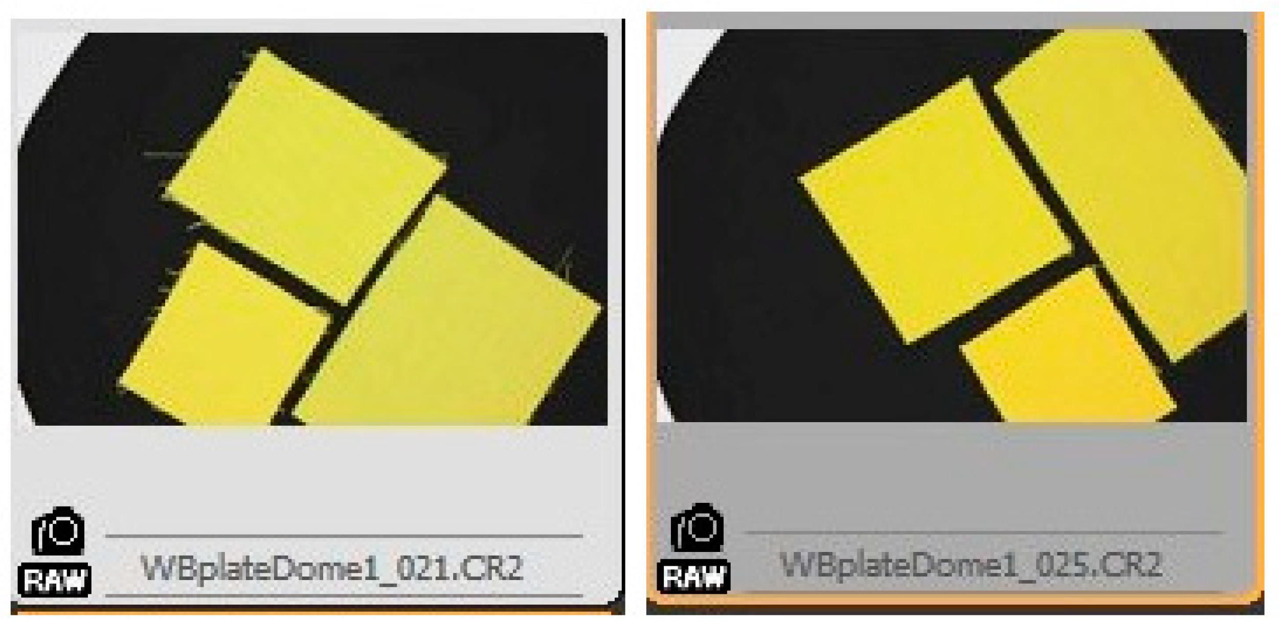
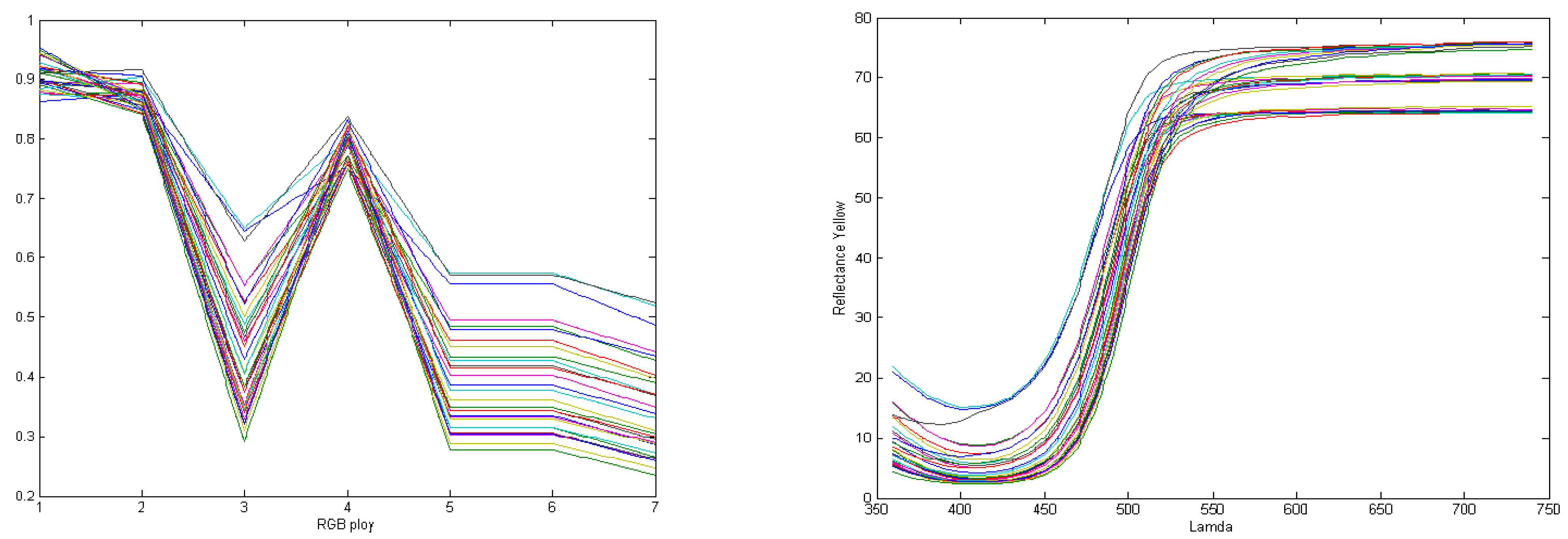
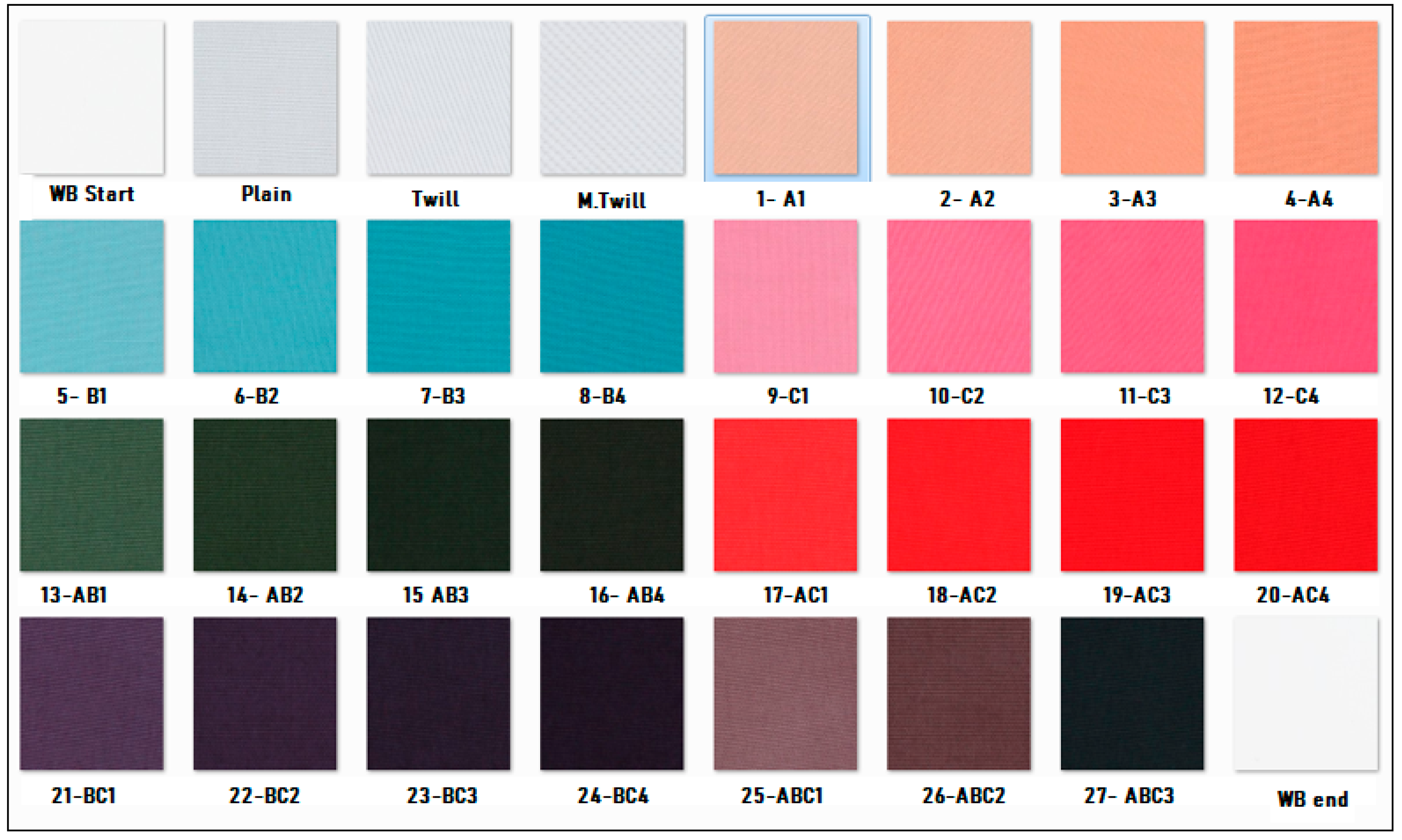
3.1. Three Types of Textures with Incremental Yellow Color Variations

Textile samples with three different textures were dyed in the same bath so that color uptake could be verified in both domains and a quantitative and qualitative analysis of color and the color difference between textiles could be conducted effectively. The integrated sphere imaging system was initially calibrated with the white plate, and all three kinds of textures dyed in the same bath were measured together (Figure 2) to ensure clarity in the determination of RGB values, denoted as Canon D450 (Camera) RGB.

Figure 3 shows the sample images and

Table 1. Experimental RGBs, color difference DE, and DERGB of three textures (Y42 as reference).

Image Plain	R	G	B	L	a	b	DERGB	DE
Y42	204.533	209.373	157.184	82.264	−10.591	40.672	0.000	0.000
Y45	208.447	207.940	135.769	81.522	−11.025	52.999	21.817	12.357
Y48	209.246	207.691	130.600	81.427	−10.942	56.523	27.051	15.877
Y51	210.326	206.055	121.697	80.914	−10.662	61.406	36.109	20.778
Y54	211.899	205.708	116.833	80.870	−10.024	64.534	41.182	23.910
Y55	217.369	207.660	109.919	82.483	−9.235	70.781	49.007	30.141
Y58	219.379	205.177	99.177	82.355	−8.232	75.616	60.023	35.024
Y61	219.503	203.863	95.189	82.013	−7.573	76.966	64.015	36.420
Y64	219.910	201.003	88.265	81.746	−7.075	79.624	71.108	39.114
Y67	221.463	201.337	85.567	81.241	−6.406	81.147	74.028	40.704
Y70	221.886	199.651	80.806	80.811	−5.926	82.224	78.926	41.839
Image Twill	R	G	B	L	a	b	DERGB	DE
Y43	213.043	212.648	157.694	84.994	−10.574	43.934	9.132	4.254
Y46	214.214	211.979	136.878	84.005	−10.878	56.473	22.646	15.899
Y49	213.269	208.123	126.858	83.784	−10.610	62.748	31.584	22.129
Y52	215.311	209.160	120.162	82.911	−10.050	66.032	38.559	25.374
Y56	221.901	208.694	107.559	84.147	−7.277	75.269	52.581	34.807
Y59	225.645	204.784	91.718	83.460	−5.961	80.494	68.939	40.108
Y62	224.473	202.668	88.074	83.045	−5.239	82.006	72.241	41.686
Y65	226.816	201.740	84.951	82.349	−4.162	82.504	75.977	42.324
Y68	227.116	198.948	81.704	82.181	−3.247	82.999	79.473	42.960
Y71	226.662	195.977	75.430	81.522	−2.684	85.341	85.749	45.370
Image M. Twill	R	G	B	L	a	b	DERGB	DE
Y44	217.647	216.200	152.434	87.016	−10.600	48.633	15.528	9.271
Y47	218.018	213.410	129.578	85.588	−9.775	63.200	30.987	22.787
Y50	218.583	212.677	124.088	85.232	−9.178	68.215	36.107	27.739
Y53	219.456	210.864	115.429	84.960	−8.427	70.903	44.367	30.428
Y57	213.761	202.186	102.455	80.302	−8.790	71.804	55.965	31.246
Y60	213.628	200.362	96.945	79.861	−8.503	73.383	61.585	32.866
Y63	215.491	201.274	95.167	79.881	−8.519	73.122	63.496	32.604
Y66	215.868	199.699	89.600	79.372	−7.628	76.591	69.208	36.157
Y69	214.343	195.389	84.453	78.937	−7.086	78.145	74.710	37.784

shows the experimental RGB and color difference DE (root mean square difference of CIE L*a*b*) and DERGB (calculated as root mean square difference of R, G, and B), using the first plain weaved sample Y2 as a reference.

In both domains, their spectral and derived imaging RGB polynomials are profound. A visual difference is observed in the higher wavelength ranges of red and green (1-r, 2-g, and so on in the RGB polynomial graph in Figure 4).

3.2. Color Difference for Human Perception

From Figure 4 and Table 1, it can be observed that the textures can be visually distinguished into 3 families: plain, twill, and modified twill. The highest was M.Twill (on top), followed by Twill (middle), and the least was plain (below). The same trend can be seen by observing CIE L* values in the spectral domain as well as intensity values (R+G+B/3) in the calibrated imaging domain in Figure 7. The color difference can be distinguished much better in terms of DERGB from the proposed system than DE in CIEL*a*b* (Figure 5). It was observed that the DERGB and color difference DE readings follow obvious trends as the color concentration increases among each of the three textures. Further, we ranked all samples to compare both domains’ perception in terms of DE and DERGB.

Experimental RGBs, color difference DE, and DERGB of the textures (Y42 as reference) are given in Table 1 and plotted in Figure 5. More discrimination is noticed in the case of DERGB compared with DE. For the color perception point of view, images were ranked in terms of measured DE and estimated DERGB from images using Y42′s RGB as reference. The congruent ranks are highlighted in italic with thick borders and the flipped reading sets are in bold (color difference ranks are flipped while evaluating DE and DERGB). It can be observed that these flipped sets (Y46, Y48), (Y53, Y55), and (Y65, Y70) have closer DE values among them (0.022, 0.287, and 0.485, respectively).

If the color difference (DE) is less than 0.5, it can be perceived as the same color and we accept it for industrial applications as well [11,12]. While observing this set of samples (shown in Figure 6) carefully, it can be easily noticed that the left-side samples Y46, Y53, and Y65 may be perceived as more colored than the samples Y48, Y55, and Y70, respectively. In fact, texture clearly has a greater impact on imaging systems, whereas color spectral reflection measurement was designed for color (reflection spectra in the visible wavelength range).

Critically, these color perception mismatches, or zones of confusion, are always debated, and the errors were profoundly significant. This is because, in most cases, the imaging domain RGB parameters are derived with a lot of assumptions and a lack of calibration, illumination information, viewing geometry, etc., while being transformed from or to CIE spaces. The reason for this is that human perception models only accept the CIE system because standardization of RGB color space is near to impossible [3,13]. These theoretical errors have been reported for decades, and it is evident that the images obtained from this calibrated imaging system could be closer to our color perception and appearance due to texture change. In addition, a color image with calibrated RGBs can be much more useful than spectral ones for real-world applications. Complex algorithms for domain transfer from device-dependent systems to device-independent systems are progressively being used for various important applications, including medical imaging; however, these conversions may cause serious errors and outliers when generalized. Sciuto et al. (2017) [14] and Lo Sciuto et al. (2021) [15] reported some improved network classifiers and feature extraction algorithms for better results to recognize organic solar cells defects. The typical RGB values of standard illuminants in different device-dependent RGB spaces are given in

Table 2. Typical RGB values of standard illuminants in different device-dependent RGB spaces.

Working	Reference	Range = [0.0, 1.0]			Range = [0, 255]
Space	Illuminant	Red	Green	Blue	Red	Green	Blue
Adobe RGB (1998)	D65	0.4947	0.4219	0.4095	126	108	104
Apple RGB	D65	0.4440	0.3459	0.3347	113	88	85
Best RGB	D50	0.4933	0.4333	0.4120	126	110	105
Beta RGB	D50	0.4913	0.4270	0.4115	125	109	105
Bruce RGB	D65	0.5099	0.4219	0.4095	130	108	104
CIE RGB	E	0.5120	0.4322	0.4130	131	110	105
ColorMatch RGB	D50	0.4444	0.3454	0.3333	113	88	85
Don RGB 4	D50	0.4934	0.4285	0.4115	126	109	105
ECI RGB v2	D50	0.5319	0.4586	0.4445	136	117	113
Ekta Space PS5 RGB	D50	0.4983	0.4275	0.4114	127	109	105
NTSC RGB	C	0.4922	0.4251	0.4122	126	108	105
PAL/SECAM RGB	D65	0.5166	0.4219	0.4088	132	108	104
ProPhoto RGB	D50	0.4071	0.3599	0.3386	104	92	86
SMPTE-C RGB	D65	0.5261	0.4199	0.4092	134	107	104
sRGB	D65	0.5246	0.4233	0.4098	134	108	105
Wide Gamut RGB	D50	0.4875	0.4326	0.4109	124	110	105

. These values can be computed and were available from the spectral calculator spreadsheet by Bruce Justin Lindbloom [16], which was used later for RGB calculations and visualizations in various RGB color spaces. The application of device-dependent systems has been growing exponentially for AI, cloud computing, virtual realities, and many more. It is critical that device-independent systems like CIEL*a*b* are always associated with their illumination and observer pairs. However, image processing researchers rarely consider this and incorrectly assume many parameters for computing RGB associations for empirical models with complex algorithms.

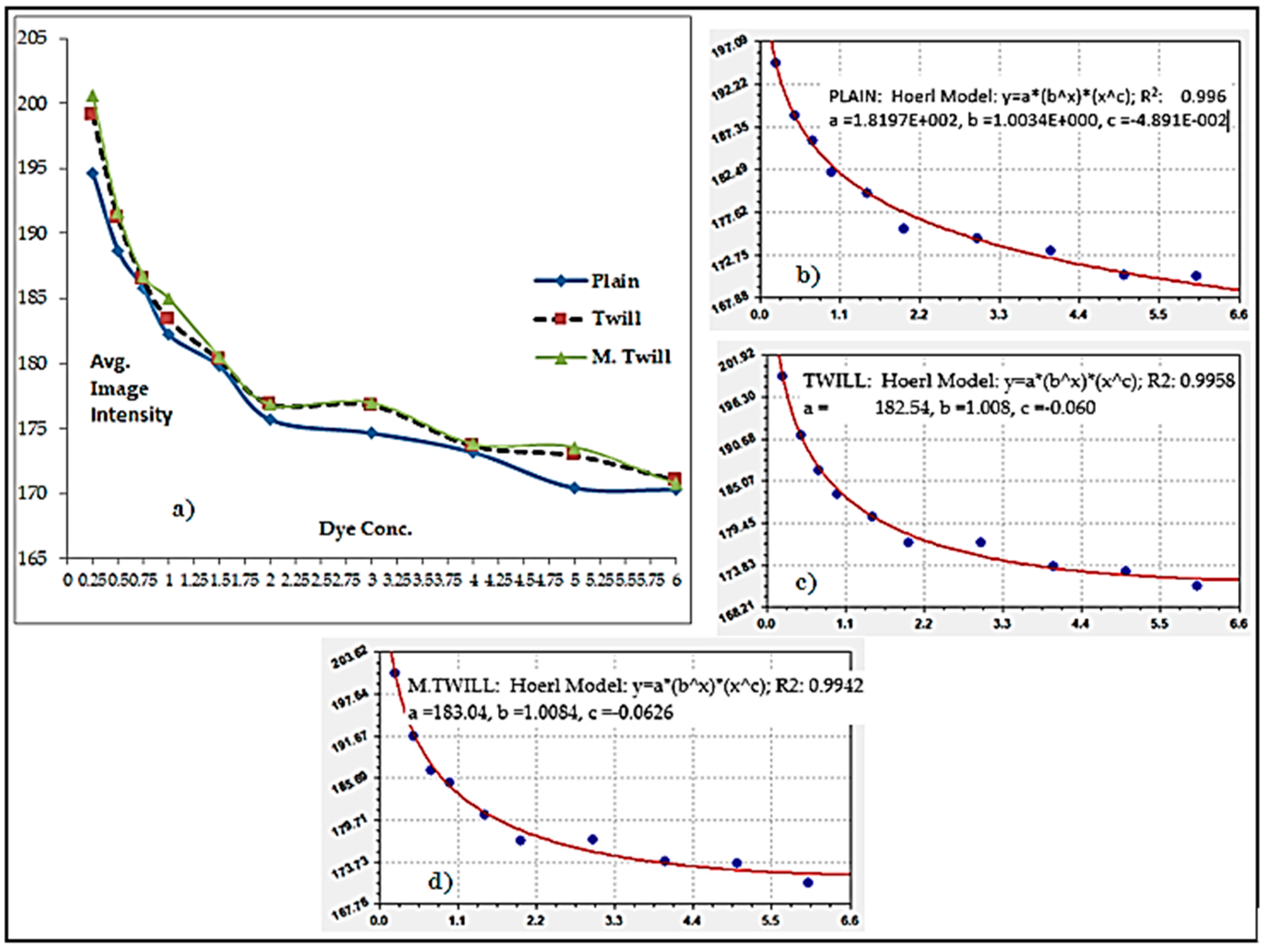
3.3. Color Intensity for Quantitative Evaluation

The intensity values were computed as (R+G+B)/3 for 10 ranges of incremental dye concentration (

Table 3. Intensity of all three textured samples with respect to 10 incremental concentration ranges.

	Dye Conc.	Plain	Twill	M. Twill
	0.25	194.656	199.113	200.631
	0.5	188.669	191.246	191.7
	0.75	185.828	186.492	186.726
	1	182.218	183.356	184.989
INTENSITY	1.5	179.798	180.277	180.537
	2	175.681	176.884	176.851
	3	174.65	176.792	177.01
	4	173.182	173.664	173.835
	5	170.434	172.941	173.575
	6	170.315	171.017	170.746

). It can be easily noticed that the estimated intensity decreases as the concentration of dye increases, which implies lower reflection properties of the surface with higher dye absorption.

The relationship between color concentration and intensity was established using quantitative evaluation (Figure 7). Here, it is relevant to investigate whether the calibrated image intensity could imitate absorbance or dye uptake (K/S), i.e., the intensity should be estimated reasonably well when the concentration is known. The measured intensities of the three textures (total of 30) were plotted against the 10 incremental concentration ranges, as shown in Figure 7, below. The Hoerl model (y = a*(bx)*(xc)) was one of the simplest and best-fitted models that we used, and the estimated values were as follows:

• PLAIN: a = 181.97, b = 1.0034, c = −0.04.891; R² = 0.996
• TWILL: a = 182.54, b = 1.008, c = −0.060; R² = 0.9958
• M.TWILL: a = 183.04, b = 1.0084, c = −0.0626 R² = 0.9942

A high coefficient of correlation was observed for all the cases (R² > 0.99), confirming a good prediction probability from calibrated imaging.

3.4. Color Combinations and Verification of Various Color Space and CIE Chromaticity Visualizations

Further, we conducted ground truth experiments with three dyes using an equal proportion of their primary, secondary, and ternary mixtures (

Table 4. Experimental RGBs of dyed samples; three dyes: primary, secondary, and ternary mixture.

	Expt. RGB				Dye Conc.
R1	G1	B1		Dye A	Dye B	Dye C
244.94	245.19	245.07	White plate Start	0	0	0
212.67	215.70	220.67	Plain	0	0	0
221.82	224.30	229.30	Twill	0	0	0
222.30	223.41	228.29	M.Twill	0	0	0
225.8854	183.092725	161.5266		1
228.9698	171.01615	145.9466		2
231.4409	157.77435	128.4438		3
229.0542	151.03805	120.8743		4
132.9036	187.883875	199.5574			1
103.2905	171.487225	186.7164			2
81.85803	154.90475	171.7595			3
68.36905	147.47215	165.4398			4
226.5088	143.528725	168.8932				1
237.1594	109.479525	143.0099				2
237.0265	93.90495	128.7294				3
237.1948	76.637475	114.6642				4
66.98825	86.420775	68.52315		1	1
42.9088	54.638625	40.33238		2	2
32.21978	40.2767	31.8978		3	3
33.49718	37.416775	31.14613		4	4
236.8776	47.72975	53.10033		1		1
228.1448	32.008575	40.05553		2		2
219.2528	22.077875	32.17638		3		3
216.452	20.80095	30.01298		4		4
75.47473	56.261325	81.50173			1	1
51.27668	37.812475	56.64295			2	2
40.11753	31.79935	45.60925			3	3
34.06043	26.35805	38.14755			4	4
122.5145	90.82425	96.30858		0.5	0.5	0.5
88.75988	60.102025	62.1925		1	1	1
28.35833	33.9254	37.27445		2	2	2
245.04	245.13	245.36	White plate end

: Dye A -Ultra-RGB Carmen, Dye -B - Ultra-RGB Navy Blue, Dye -C: Ultra-RGB Red.

and Figure 8). Various color space RGB representations of the dye mixtures (BC at 1, 2, 3, and 4%) were computed [14] and represented in Figure 9.

The reflectance measurement was conducted using spectrophotometry, and calibrated imaging RGBs were calculated in MATLAB. The spreadsheet by Bruce Justin Lindbloom was used to calculate various device-dependent RGB standards, and all raw data were provided on an Excel file. Typical binary combinations of 1, 2, 3, and 4% of Dye B and Dye C for three major color space RGB representations (Apple RGB, Adobe RGB, and Pro-photo RGB) are given in Figure 9. It is evident that they could be well represented in both qualitative and quantitative analyses (curves of the same family have similar spectral reflectance). In addition, we investigated the similarity of their representations in the CIE chromaticity (CIExy) diagram (Figure 10) and the 3D representation of linearity of individual and dye mixtures in both domains (Figure 11). The physical significance of this is that a two-dye mixture in a particular proportion will be in a straight line until it becomes saturated.

These experimental findings demonstrate that both qualitative and quantitative evaluations are possible in the calibrated digital domain and that they are comparable to spectral or device-independent systems. The calibrated red, green, blue, RG, RB, GB, and RGB polynomial expansion can be treated as an alter ego of spectral responses for any color space, including dye mixtures, for practical applications. The CIE XYZ and 3D RGB trends revealed the distinct dye and combination profiles.

3.5. Reflectance Prediction in Terms of Calibrated RGB Polynomial Regression

As we discussed how the proposed RGB polynomial could potentially be used as an alter ego for the reflectance function earlier, we investigated further how well the reflectance function (31 values over a visible wavelength of 400–700 nm with a 10 nm gap) could be predicted. It is logical that the mixture of primary RGBs generates a wide gamut of colors. Here we have taken these 27 dye mixture samples in a similar fashion to how the database is prepared for computer color matting for prediction. It can be mathematically denoted as follows:

$$R\left(\lambda \right)=f\left(RGBpolynomial\right)$$

We used 3, 8, 11, 20, and 23 argument coefficients here, and did not try more arguments as they caused more complexity and predilection in our earlier investigation [5,17,18]. The predicted reflectance were then converted into theoretical CIEL*a*b* for various illuminant–observer pairs to calculate the predicted DE. All the experimental data (actual and predicted reflectance, coefficients, and DE) for various illuminat–observer pairs are provided as a Supplementary File. Figure 12 clearly shows that the reflectance function is well predicted from the 23-argument polynomial RGB. The arguments for the polynomial RGB function are denoted below.

Table 5. DE from predicted reflectance for D65_64.

D65_64	3 coeff	8 coeff	11 coeff	20 coeff	23 Coeff
DE Avg	2.3401	1.5	1.3221	0.4106	0.3072
DE Max	4.0535	2.72	2.9029	1.0776	1.0373
DE Min	0.8291	0.4039	0.0873	0.1007	0.0595
DE std	0.848	0.7361	0.7566	0.2691	0.2486

illustrates the summary of color difference results based on these 5 RGB polynomial arguments were derived from the predicted reflectance values. In Figure 12a the experimental reflectance was plotted as continuous line and predicted reflectance of 23 argument model was marked as *.

• 3: R G B
• 8: R G B R×G×B R×G R×B G×B 1
• 11: R G B R×G×B R×G R×B G×B R2 G2 B2 1
• 20: R G B R×G×B R×G R×B G×B R2 G2 B2 R3
• G3 B3 G×R2 B×G2 R×B2 B×R2 R×G2 G×B2 1
• 23: R G B R×G×B R×G R×B G×B R2 G2 B2
• R3 G3 B3 G×R2 B×G2 R×B2 B×R2 R×G2 G×B2
• G×B×R2 B×R×G2 R×G×B2 1

4. Conclusions

In fact, exact spectral reconstruction is even more difficult to achieve. These challenges can be easily understood if we revisit the development of CIE systems themselves with defined illuminants, observer functions (cleverly designed with real-time inputs from expert human observers), and viewing geometry set-ups. For example, we need to predict 31 values (%R from 400–700 nm in a 10 nm gap) from three colorimetric readings of CIE L*, a*, and b*. The systems required to do this are well established and being utilized for specific domain applications as of today, unlike RGBs; those are being evolved for use in pleasant images with less know-how.

In current practice, the transformation of device-dependent imaging parameters into device-independent CIE parameters is mandatory as human perception only accepts the CIE system. Before pre- and post-processing of the color images in compressed digital color space or to map specific RGBs to a specific spectrophotometer or colorimetric reading under a certain illuminant and observer, domain knowledge is a definite prerequisite. Specifically, the color and appearance perception mismatches, or zones of confusion, are being critically debated in real-world applications. In fact, humans can differentiate more colors than CIEs. The fundamental cause of these errors was profoundly significant for critical decision-making applications when imaging domain parameters with a lot of assumptions and a lack of calibration, illumination information, uniformity, etc., were transformed to CIE spaces.

Previously, we proposed an alternative reflectance function obtained from the calibrated sphere imaging system with a theoretical explanation to analyze and validate the close proximity of texture and color. Here, with three different textures and the incremental color depth of three color combinations, we experimented and validated the qualitative analysis of color and proximity texture in both domains. The concentration of a particular color can be estimated from the calibrated image intensity. The human perception of color differences and its ambiguity are explained. The color difference in terms of DERGB can be perceived well and texture has a large influence on it. The reflectance predictions from polynomial regression RGB models were found to be reasonably accurate. The various RGB spaces and CIExyz for color combinations were found to be congruent, and finally, precision can be ensured if an image is well calibrated with diffused and uniform illumination constancy.

References

1. Rout, N.; Baciu, G.; Pattanaik, P.; Nakkeeran, K.; Khandual, A. Color and Texture Analysis of Textiles Using Image Acquisition and Spectral Analysis in Calibrated Sphere Imaging System-I. Electronics 2022, 24, 3887. [Google Scholar] [CrossRef]
2. Yao, P. Advanced Textile Image Analysis Based on Multispectral Color Reproduction. Ph.D. Dissertation, Hong Kong Polytechnic University, Hong Kong, China, 2022. [Google Scholar]
3. Khandual, A.; Baciu, G.; Rout, N. Colorimetric processing of digital color image! Int. J. Adv. Res. Comp. Sc. Soft. Eng. 2013, 3, 103–107. [Google Scholar]
4. Zhang, J.; Su, R.; Fu, Q.; Ren, W.; Heide, F.; Nie, Y. A survey on computational spectral reconstruction methods from RGB to hyperspectral imaging. Sci. Rep. 2022, 12, 11905. [Google Scholar] [CrossRef] [PubMed]
5. Khandual, A.; Baciu, G.; Hu, J.; Zeng, E. Color Characterization for Scanners: Dpi and Color Co-Ordinate Issues. Int. J. Adv. Res. Comput. Sci. Softw. Eng. 2012, 2, 354–365. [Google Scholar]
6. Ershov, E.; Savchik, A.; Shepelev, D.; Banić, N.; Brown, M.S.; Timofte, R.; Mudenagudi, U. NTIRE 2022 challenge on night photography rendering. In Proceedings of the IEEE/CVF Conference on Computer Vision and Pattern Recognition, New Orleans, LA, USA, 18–24 June 2022; pp. 1287–1300. [Google Scholar]
7. Nayak, S.; Khandual, A.; Mishra, J. Ground truth study on fractal dimension of color images of similar texture. J. Text. Inst. 2018, 109, 1159–1167. [Google Scholar] [CrossRef]
8. Nie, C.; Xu, C.; Li, Z.; Chu, L.; Hu, Y. Specular reflections detection and removal for endoscopic images based on brightness classification. Sensors 2023, 23, 974. [Google Scholar] [CrossRef] [PubMed]
9. Abdulateef, S.K.; Hasoon, A.N. Comparison of the components of different color spaces to enhanced image representation. J. Image Process. Intell. Remote Sens. 2023, 3, 11–17. [Google Scholar]
10. Lin, Y.T.; Finlayson, G.D. An investigation on worst-case spectral reconstruction from RGB images via Radiance Mondrian World assumption. Color Res. Appl. 2023, 48, 230–242. [Google Scholar] [CrossRef]
11. Gupte, V.C. Color Technology: Tools, Techniques and Applications; Woodhead Publishing: Sawston, UK, 2008. [Google Scholar]
12. Kandi, S.G. The Effect of Spectrophotometer Geometry on the Measured Colors for Textile Samples with Different Textures. J. Eng. Fibers Fabr. 2011, 6, 70–78. [Google Scholar] [CrossRef]
13. Süsstrunk, S.; Buckley, R.; Swen, S. Standard RGB color spaces. In Proceedings of the IS&T;/SID 7th Color Imaging Conference, Lausanne, Switzerland, 16–19 November 1999; pp. 127–134. [Google Scholar]
14. Sciuto, G.L.; Capizzi, G.; Gotleyb, D.; Linde, S.; Shikler, R.; Woźniak, M.; Połap, D. Combining SVD and co-occurrence matrix information to recognize organic solar cells defects with a elliptical basis function network classifier. In Proceedings of the Artificial Intelligence and Soft Computing: 16th International Conference, ICAISC 2017, , Proceedings, Part II 16, Zakopane, Poland, 11–15 June 2017; Springer International Publishing: Berlin/Heidelberg, Germany; pp. 518–532. [Google Scholar]
15. Lo Sciuto, G.; Capizzi, G.; Shikler, R.; Napoli, C. Organic solar cells defects classification by using a new feature extraction algorithm and an EBNN with an innovative pruning algorithm. Int. J. Intell. Syst. 2021, 36, 2443–2464. [Google Scholar] [CrossRef]
16. Bruce Justin Lindbloom’s Spectral Calculator Spreadsheet. Available online: http://www.brucelindbloom.com/ (accessed on 1 March 2023).
17. Khandual, A.; Baciu, G.; Hu, J.; Zheng, D. Colour characterization for scanners: Validations on Textiles & Paints. Int. J. Adv. Res. Comput. Sci. Softw. Eng. 2001, 3, 1008–1013. [Google Scholar]
18. Baciu, G.; Khandual, A.; Hu, J.; Xin, B. Device and Method for Testing Fabric Color. CN 101788341 B Patent 1 October 2012. [Google Scholar]
Figure 1. A typical % reflectance and K/S profile of ultra orange RGB dye.
Electronics 12 02135 g001
Figure 2. Measurement of three textures together in a calibrated integrated sphere imaging system.
Electronics 12 02135 g002
Figure 3. Incremental yellow dyed samples for three textures.
Electronics 12 02135 g003aElectronics 12 02135 g003b
Figure 4. Spectral and RGB polynomial representations of all 30 yellow samples.
Electronics 12 02135 g004
Figure 5. DERGB and DE of three textures, dyed with yellow in the same bath.
Electronics 12 02135 g005
Figure 6. Image ranking according to the color difference DE and DERGB for all 30 samples.
Electronics 12 02135 g006
Figure 7. Intensity average vs. dye concentrations (a) of all 30 yellow samples; Hoerl model fit for (b) plain weave, (c) twill weave, and (d) modified twill weave.
Electronics 12 02135 g007
Figure 8. Images of the dyed samples; three dyes: primary, secondary, and ternary mixture.
Electronics 12 02135 g008
Figure 9. Various color space RGB representations of the dye mixture (BC at 1, 2, 3, and 4%).
Electronics 12 02135 g009
Figure 10. CIExy diagram for all 27 color combinations.
Electronics 12 02135 g010
Figure 11. 3D Plots of CIExyz and RGBs of all 27 dyed samples.
Electronics 12 02135 g011
Figure 12. (a) Reflectance functions of 27 samples predicted from a 23-argument RGB polynomial. It is noteworthy that these reflectance models would be more accurate in cases where we use the same substrate and dye combinations and it is highly probable that their predictions would ensure non-metameric matches for all sets of ASTM illuminant–observer pairs. The experimental and predicted CIE L*a*b* are plotted in (bd). (b) CIE L* vs. Lp*, (c) CIE a* vs. ap*, and (d) CIE b* vs. bp*.
Electronics 12 02135 g012aElectronics 12 02135 g012b