Resolution-Enhanced and Accurate Cascade Time-Reversal Operator Decomposition (C-DORT) Approach for Positioning Radiated Passive Intermodulation Sources

Abstract

Attaining a high-resolution and accurate location for a radiated passive intermodulation source (R-PIMS) has been an increasingly interesting problem in modern multi-carrier wireless communication systems. For precisely positioning multiple closely spaced R-PIMSs, a novel imaging method called cascade decomposition of time-reversal operator (C-DORT) was developed. C-DORT constructs a new spectrum calculation by normalizing and multiplying the pseudo-spectrum at each sampled frequency together. The cascade process focuses the pseudo-spectrum at R-PIMS positions to form a highly brightened spectrum peak and to suppress the remained pseudo-spectrum to approximately zero, contributing to distinguishing the closely spaced R-PIMSs. The positioning performance of the positioning resolution, pseudo-spectrum width, positioning accuracy, and imaging robustness are analyzed by numerical simulations. Compared with the conventional central frequency decomposition of time-reversal operator (CF-DORT) and the time domain decomposition of time-reversal operator (TD-DORT) methods, the multiple R-PIMSs, spaced at a distance of diffraction limit, which is the spacing of 1/2 of a wavelength, are distinguished effectively in C-DORT. Additionally, the cross-range pseudo-spectrum full width at half maxima (CRPS-FWHM) is suppressed to the width of 1/4 of a wavelength by multiplication to improve the cross-range resolution in C-DORT. In addition, accurate positioning is obtained by providing the approximately zero positioning root mean square estimation (RMSE) at an SNR ranging from 0 dB to 10 dB. The results show that the proposed C-DORT improves the positioning accuracy and enhances the positioning resolution for locating an R-PIMS.

1. Introduction

Facing to the application demands of sixth-generation (6G) wireless communication and future satellite internet, modern wireless systems are developing into multi-carrier systems with a wide bandwidth, high power, large capacity and high communication rate [1]. Passive intermodulation (PIM) has been an increasingly tough problem in such wireless systems with great emitted power and a multi-carrier signal [2,3]. Generally, PIM can be classified into conducted passive intermodulation (C-PIM) and radiated passive intermodulation (R-PIM) [4]. C-PIM usually exists in the passive devices and radio frequency (RF) components, which include duplexers, coaxial connectors, and waveguide flanges [5,6,7]. The C-PIM interferent signals are generated at the junctions and propagate forward and backward along the wave-guided RF chains [8,9]. R-PIM is radiated by the radiation structures, such as antennas and scatterers nearby [1]. The R-PIM positions are excited by the radiation structures and radiated to the medium, which can be regarded as the secondary radiated sources and can be called the radiated passive intermodulation sources (R-PIMSs). Due to the complicated components and structures in a wireless system, attaining an accurate and high-resolution location for R-PIMS has been a tough and challenging problem.

Due to its good spatiotemporal focusing property in complicated environments, the time reversal (TR) technique has been widely used in detecting and imaging applications, such as medical imaging [10,11], microwave imaging [12], radar imaging [13,14], and damage detection [15]. For the fundamental TR imaging technique, iterative time-reversal mirror (ITRM) imaging method works by iteratively retransmitting the back-scatterer signals and realizes the scatterer’s positioning in the medium [16]. However, the ITRM method is exposed to overwhelm from the weak-amplitude target and cannot distinguish between a far target and a near target. To selectively image each target in TR imaging methods, the time-reversal operator (TRO) imaging methods were developed and proposed in previous decades [17,18,19,20]. Selective imaging is realized by extracting the significant eigenvalue distribution and corresponding eigenvector from the TRO decomposition. Generally, significant eigenvalues are mapped to the number of the detected targets, and the corresponding eigenvector of each eigenvalue is relevant with the located information. Hence, one may choose the specific eigenvector corresponding to each significant eigenvalue to realize the selective imaging for each target in the TRO imaging methods. The TRO is constructed by a multi-static data matrix (MDM), which can also mainly be classified into two categories: the space–space multi-static data matrix (SS-MDM) and the space-frequency multi-static data matrix (SF-MDM) [21,22].

Based on the TRO built by the SS-MDM, the signal subspace and noise subspace are decomposed via singular value decomposition (SVD). The signal subspace and noise subspace are employed to have a correlative operation with the transmission matrix in an imaging region. Then, the decomposition of the time-reversal operator (DORT) approach and time-reversal multiple signals classification (TR-MUSIC) method [23,24] are employed. To further enhance the imaging accuracy, the bandwidth of the imaging system is extended into wideband or ultrawideband (UWB). Hence, the central frequency decomposition of the time-reversal operator (CF-DORT), the central frequency time-reversal multiple signals classification (CF-TR-MUSIC), the time domain decomposition of the time-reversal operator (TD-DORT), and UWB-TR-MUSIC methods are developed [25,26]. Though CF-TR-MUSIC and UWB-TR-MUSIC can distinguish the multiple closely spaced targets, they are sensitive to the noise, while CF-DORT and TD-DORT have a better anti-noise performance [27,28]. Differing from the SS-MDM, the row vector of the SF-MDM denotes the frequency information for each antenna element, and the column vector of SF-MDM represents the spatial information for each sampled frequency. Based on the SF-MDM, selective TR imaging methods are also developed [29,30,31]. Additionally, other derived MDMs, such as a frequency–frequency multi-static data matrix (FF-MDM) for selectively positioning targets, are also presented [32].

In general, based on different MDMs, the aforementioned TR subspace methods can be classified into TR-MUSIC-based methods and DORT-based methods. DORT-based methods have a good ability to tolerate a noisy environment, but their positioning resolution is limited and must be improved.

In this paper, the cascade decomposition of the time-reversal operator (C-DORT) imaging method to realize the location for multiple R-PIMSs spaced at less than the diffraction limit is discussed. In the C-DORT method, the normalization and multiplication for the DORT spectra at each sampled frequency are called cascade processes. Different from the traditional pseudo-spectrum in the CF-DORT or TD-DORT approaches, through the cascade process in the C-DORT method, the pseudo-spectrum around the R-PIMS is squeezed and brightened, and the widths of the pseudo-spectrum in the C-DORT method are also reduced. Moreover, the remaining pseudo-spectrum is suppressed to approximately zero. These contribute to improving the accuracy of positioning R-PIMSs and enhancing the positioning resolution in the positioning of closely spaced multiple R-PIMSs.

2. Signal Model and DORT-Based Methods

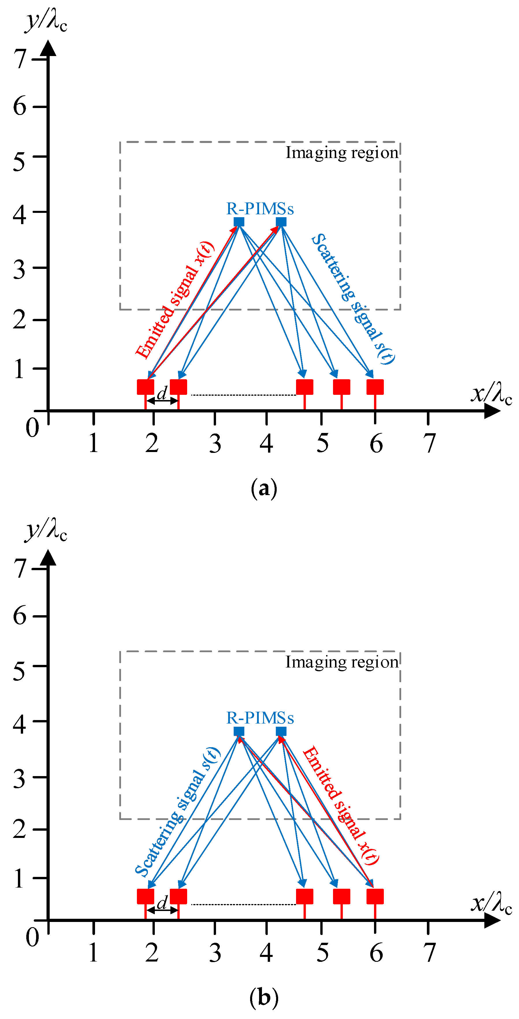
2.1. Signal Model

Figure 1 illustrates the schematic for positioning multiple R-PIMSs targets. In these figures, the M azure dice are denoted as the R-PIMSs. It should be noted that the R-PIMSs are randomly located inside the imaging region, and their positions are unknown. However, the positions of the R-PIMSs are still assumed as ${\mathit{r}}_M\left(M=1,2\dots M\right)$. The red dice represent the antenna elements of the linear antenna array for positioning these R-PIMSs. The detecting antenna array, which harvests the scattering signals from the R-PIMSs, is constructed with the L antenna elements, which are located along with the x axis. These array elements are located at ${\mathit{r}}_L\left(L=1,2\dots L\right),$ and the spacing between two adjust elements is $d={\lambda }_{\mathrm{c}}/2$, where ${\lambda }_{\mathrm{c}}$ is the wavelength of the signal central frequency ${\omega }_{\mathrm{c}}$.

Assume that each emitted signal from each antenna element is denoted as $x\left(t\right)$; the total harvested signals of antenna array can be obtained as

$$S\left(t\right)=H\left(t\right)\otimes x\left(t\right)$$

(1)

where $S\left(t\right)$ is the time signal matrix of the dimension $L\times L$, and $\otimes$ is a convolution operator. The scattering signals excited by the first antenna element and by the last antenna element are harvested by the antenna arrays, $s_1\left(t\right)={\left[s_{11}\left(t\right),s_{21}\left(t\right),\dots ,s_{L1}\left(t\right)\right]}^{\mathrm{T}}$ and $s_L\left(t\right)={\left[s_{1L}\left(t\right),s_{2L}\left(t\right),\dots ,s_{LL}\left(t\right)\right]}^{\mathrm{T}}$ in Figure 1a,b, respectively. Namely, combined with (1), the $S\left(t\right)$ harvested for each excitation is constructed by

$$S\left(t\right)=\left[\begin{array}{cc}\begin{array}{cc}{s}_{11}\left(t\right)& s_{12}\left(t\right)\\ s_{21}\left(t\right)& s_{22}\left(t\right)\end{array}& \begin{array}{cc}\cdots & s_{1L}\left(t\right)\\ \cdots & s_{2L}\left(t\right)\end{array}\\ \begin{array}{cc}⋮& ⋮\\ s_{L1}\left(t\right)& s_{L2}\left(t\right)\end{array}& \begin{array}{cc}\ddots & ⋮\\ \cdots & s_{LL}\left(t\right)\end{array}\end{array}\right]=\left[\begin{array}{cc}\begin{array}{cc}{h}_{11}\left(t\right)& h_{12}\left(t\right)\\ h_{21}\left(t\right)& h_{22}\left(t\right)\end{array}& \begin{array}{cc}\cdots & h_{1L}\left(t\right)\\ \cdots & h_{2L}\left(t\right)\end{array}\\ \begin{array}{cc}⋮& ⋮\\ h_{L1}\left(t\right)& h_{L2}\left(t\right)\end{array}& \begin{array}{cc}\ddots & ⋮\\ \cdots & h_{LL}\left(t\right)\end{array}\end{array}\right]\otimes x\left(t\right)$$

(2)

where the $s_{ij}\left(t\right)$ is such that the ith antenna element receives the scattering signals by the jth excitation, and $h_{ij}\left(t\right)$ represents the mixed impulse response between the R-PIMSs and the ith antenna element by the jth excitation. Based on the reciprocal theory, $h_{ij}\left(t\right)=h_{ji}\left(t\right)$.

By the Fourier transformation, $S\left(t\right)$ can be transformed into the frequency domain as

$$S\left({\omega }_k\right)=H\left({\omega }_k\right)x\left({\omega }_k\right)=\left[\begin{array}{cc}\begin{array}{cc}{h}_{11}\left({\omega }_k\right)& h_{12}\left({\omega }_k\right)\\ h_{21}\left({\omega }_k\right)& h_{22}\left({\omega }_k\right)\end{array}& \begin{array}{cc}\cdots & h_{1L}\left({\omega }_k\right)\\ \cdots & h_{2L}\left({\omega }_k\right)\end{array}\\ \begin{array}{cc}⋮& ⋮\\ h_{L1}\left({\omega }_k\right)& h_{L2}\left({\omega }_k\right)\end{array}& \begin{array}{cc}\ddots & ⋮\\ \cdots & h_{LL}\left({\omega }_k\right)\end{array}\end{array}\right]x\left({\omega }_k\right)$$

(3)

where ${\omega }_k\left(k=1,2,\dots K\right)$ is the kth frequency uniformly sampled in the operating frequency bandwidth. $S\left({\omega }_k\right)$, $H\left({\omega }_k\right),$ and $x\left({\omega }_k\right)$ are the Fourier transforms of the $S\left(t\right)$, $H\left(t\right),$ and $x\left(t\right)$, respectively. As the emitted signal $x\left(t\right)$ by each excitation is consistent, the frequency signal transfer matrix $H\left({\omega }_k\right)$ can be extracted as

$$H\left({\omega }_k\right)=\left[\begin{array}{cc}\begin{array}{cc}{h}_{11}\left({\omega }_k\right)& h_{12}\left({\omega }_k\right)\\ h_{21}\left({\omega }_k\right)& h_{22}\left({\omega }_k\right)\end{array}& \begin{array}{cc}\cdots & h_{1L}\left({\omega }_k\right)\\ \cdots & h_{2L}\left({\omega }_k\right)\end{array}\\ \begin{array}{cc}⋮& ⋮\\ h_{L1}\left({\omega }_k\right)& h_{L2}\left({\omega }_k\right)\end{array}& \begin{array}{cc}\ddots & ⋮\\ \cdots & h_{LL}\left({\omega }_k\right)\end{array}\end{array}\right]$$

(4)

Considered that Gaussian white noise is in the received signals, the frequency signal transfer matrix $H_N\left({\omega }_k\right)$ can be obtained as

$$H_N\left({\omega }_k\right)=H\left({\omega }_k\right)+N\left({\omega }_k\right)$$

(5)

where $N\left({\omega }_k\right)$ is the Gaussian white noise matrix of a dimension of $L\times L$. Following the TRO in Equation (5), the basic imaging principles of CF-DORT, TD-DORT, and the proposed C-DORT are compared, and they are collectively called the DORT-based method.

2.2. CF-DORT

In conventional TR imaging methods, the CF-DORT is dependent on the TRO at the central frequency of the operating bandwidth, which is defined as

$$T\left({\omega }_c\right)={\left(H_N\left({\omega }_c\right)\right)}^{\mathrm{H}}{H}_N\left({\omega }_c\right)$$

(6)

where ${( )}^{\mathrm{H}}$ is the Hermitian transpose operator, and $T\left({\omega }_c\right)$ is a $L\times L$ square matrix. The SVD for $T\left({\omega }_c\right)$ is as following

$$T\left({\omega }_c\right)=U\left({\omega }_c\right)\Lambda \left({\omega }_c\right){\left(V\left({\omega }_c\right)\right)}^{\mathrm{H}}$$

(7)

$\Lambda \left({\omega }_c\right)$ is the $L\times L$ singular-value real diagonal matrix, and their singular values are distributed as ${\lambda }_1\left({\omega }_{\mathrm{c}}\right),{\lambda }_2\left({\omega }_{\mathrm{c}}\right),\dots ,{\lambda }_L\left({\omega }_{\mathrm{c}}\right)$. The corresponding eigenvectors ${\mu }_1\left({\omega }_{\mathrm{c}}\right),{\mu }_2\left({\omega }_{\mathrm{c}}\right),\dots ,{\mu }_L\left({\omega }_{\mathrm{c}}\right)$ are spanned as matrix $U\left({\omega }_c\right)$. The eigenvectors $\left[{\mu }_i\left({\omega }_{\mathrm{c}}\right),i=1,2,\dots ,M\right]$ correspond to the M significant eigenvalues, while the eigenvectors $\left[{\mu }_i\left({\omega }_{\mathrm{c}}\right),i=M+1,M+2,\dots ,L\right]$ are correspond to the $L-M$ small significant eigenvalues. Moreover, the M significant eigenvalues are spanned to the signal subspace, while the $L-M$ small eigenvectors are spanned to the noise subspace. Theoretically, the number of ideal, point-like R-PIMS targets is equal to M, and each eigenvector in signal subspace corresponds to each R-PIMS target.

From the decomposition of the TRO, a number of targets less than that of the antenna elements is required. The phase of an eigenvector in signal subspace is consistent to that of a signal vector at the position of the R-PIMS target. Hence, the pseudo-spectrum calculation of the CF-DORT for each R-PIMS target is obtained, and the image function of all the R-PIMS targets can be written by:

$$I_{CF-DORT}\left(r_{se}\right)={\displaystyle \sum }_{m=1}^M\langle g\left(r_{se},{\omega }_{\mathrm{c}}\right),{\left({\mu }_m\left({\omega }_{\mathrm{c}}\right)\right)}^{*}\rangle$$

(8)

where $r_{\mathrm{se}}$ is the searching point in the imaging region, and $g\left(r_{se},{\omega }_{\mathrm{c}}\right)$ are the transmission vectors between the searching point and the antenna array. The ${( )}^{*}$ denotes the conjugation process.

$$g\left(r_{\mathrm{se}},{\omega }_{\mathrm{c}}\right)=\left[G\left(r_1,r_{\mathrm{se}},{\omega }_{\mathrm{c}}\right),G\left(r_2,r_{\mathrm{se}},{\omega }_{\mathrm{c}}\right),\dots ,G\left(r_L,r_{\mathrm{se}},{\omega }_{\mathrm{c}}\right)\right]$$

(9)

where $G\left(r_l,r_{\mathrm{se}},{\omega }_{\mathrm{c}}\right)=e^{-j{w}_v\left({\omega }_{\mathrm{c}}\right)\left|r_l-r_{\mathrm{se}}\right|}/4\pi \left|r_l-r_{\mathrm{se}}\right|, l=1,2,\dots ,L$ is the frequency domain Green Function between the position of each antenna element $r_l$ and $r_{\mathrm{se}}$, $w_v\left(\omega \right)$ is the wave vector, and $\left|r_l-r_{\mathrm{se}}\right|$ is the distance between the position of each antenna element $r_l$ and $r_{\mathrm{se}}$.

2.3. TD-DORT

The SVD for TRO is commonly used in addition to the full-frequency bandwidth or in multiple frequencies. The back-transmission time domain signal $r{e}_m\left(t\right)$ $m=1,2,\dots ,M$ can written by

$$r{e}_m\left(t\right)=\underset{\mathsf{\Omega }}{\overset{ }{{\displaystyle \int }}}{\lambda }_m\left(\omega \right){\mu }_m\left(\omega \right)e^{j\omega t}d\omega$$

(10)

where $\mathsf{\Omega }$ is the frequency bandwidth. The $r{e}_m\left(t\right)$ is retransmitted back to the imaging region. The pseudo-spectrum calculation of the TD-DORT for each R-PIMS target is obtained, and here the image function of all the R-PIMS targets can be written by

$$I_{TD-DORT}\left(r_{se}\right)={\displaystyle \sum }_{m=1}^M\left(\underset{\mathsf{\Omega }}{\overset{ }{{\displaystyle \int }}}{\lambda }_m\left(\omega \right){\left[{\mu }_m\left(\omega \right)\right]}^{\mathrm{T}}g\left(r_{se},\omega \right)d\omega \right)$$

(11)

where ${( )}^{\mathrm{T}}$ is the transpose operator, and $g\left(r_{se},\omega \right)$ can be derived by Equation (9).

3. The Proposed C-DORT Method

Here, the new pseudo-spectrum calculation method of multiplying the spectra obtained at each uniform sampled frequency in a cascaded way is developed and called C-DORT. The pseudo-spectrum calculation of the C-DORT for each R-PIMS target is obtained, and here the image function of all the R-PIMS targets can be written by

$$I_{C-DORT}\left(r_{se}\right)={\displaystyle \sum }_{m=1}^M\left[{\displaystyle \prod }_{k=1}^K{I}_m^{\mathrm{norm}}\left(r_{se},{\omega }_k\right)\right]$$

(12)

where $I_m^{\mathrm{norm}}\left(r_{se},{\omega }_k\right)$ is obtained by

$$I_m^{\mathrm{norm}}\left(r_{se},{\omega }_k\right)=I_m\left(r_{se},{\omega }_k\right)/\max \left(I_m\left(r_{se},{\omega }_k\right)\right)$$

(13)

where $I_m\left(r_{se},{\omega }_k\right)$ is formulated as

$$I_m\left(r_{se},{\omega }_k\right)=\langle g\left(r_{se},{\omega }_k\right),{\left({\mu }_m\left({\omega }_k\right)\right)}^{*}\rangle$$

(14)

By pseudo-spectrum normalization, the pseudo-spectrum at the R-PIMS’ position is, ideally, normalized as $1$, and the others’ pseudo-spectra are suppressed to below 1. Then, multiplying the normalized pseudo-spectrum in all bandwidths can make the others’ pseudo-spectra fall below 1, gradually approaching 0. Hence, the multiplication process weakens the positions of the others on the pseudo-spectrum to improve the resolution, reduces the side lobes, and makes the R-PIMS position easier and more accurate in positioning images.

4. Simulation Results and Discussion

Based on the model in Figure 1, numerical simulations of a positioning R-PIMS were carried out. These numerical simulations operated with the $1.5 \mathrm{GHz}$ frequency bandwidth ranging from $1 \mathrm{GHz}$ to $2.5 \mathrm{GHz}$, whose central frequency is $1.75 \mathrm{GHz}$. The imaging region in Figure 1 is $9{\lambda }_{\mathrm{c}}\times 9{\lambda }_{\mathrm{c}}$, with $100\times 100$ pixels, in which ${\lambda }_{\mathrm{c}}=17.14 \mathrm{cm}$. The number of detecting antennas in the array is $L=11,$ and their distance between two adjacent antenna elements is $d=8.57 \mathrm{cm}$. For multiple-frequency DORT methods, there is a total of $K=16$ uniform sampled frequencies.

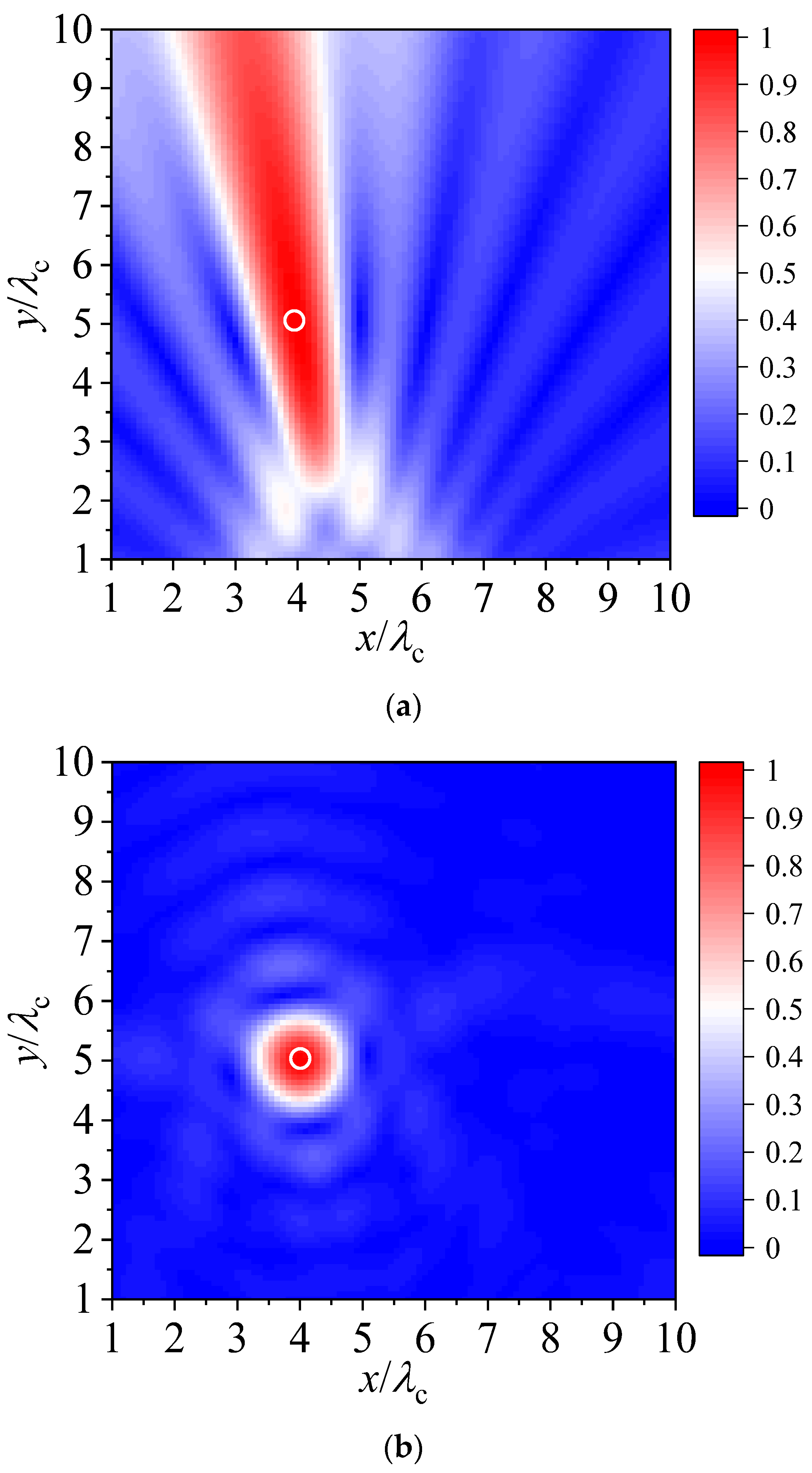
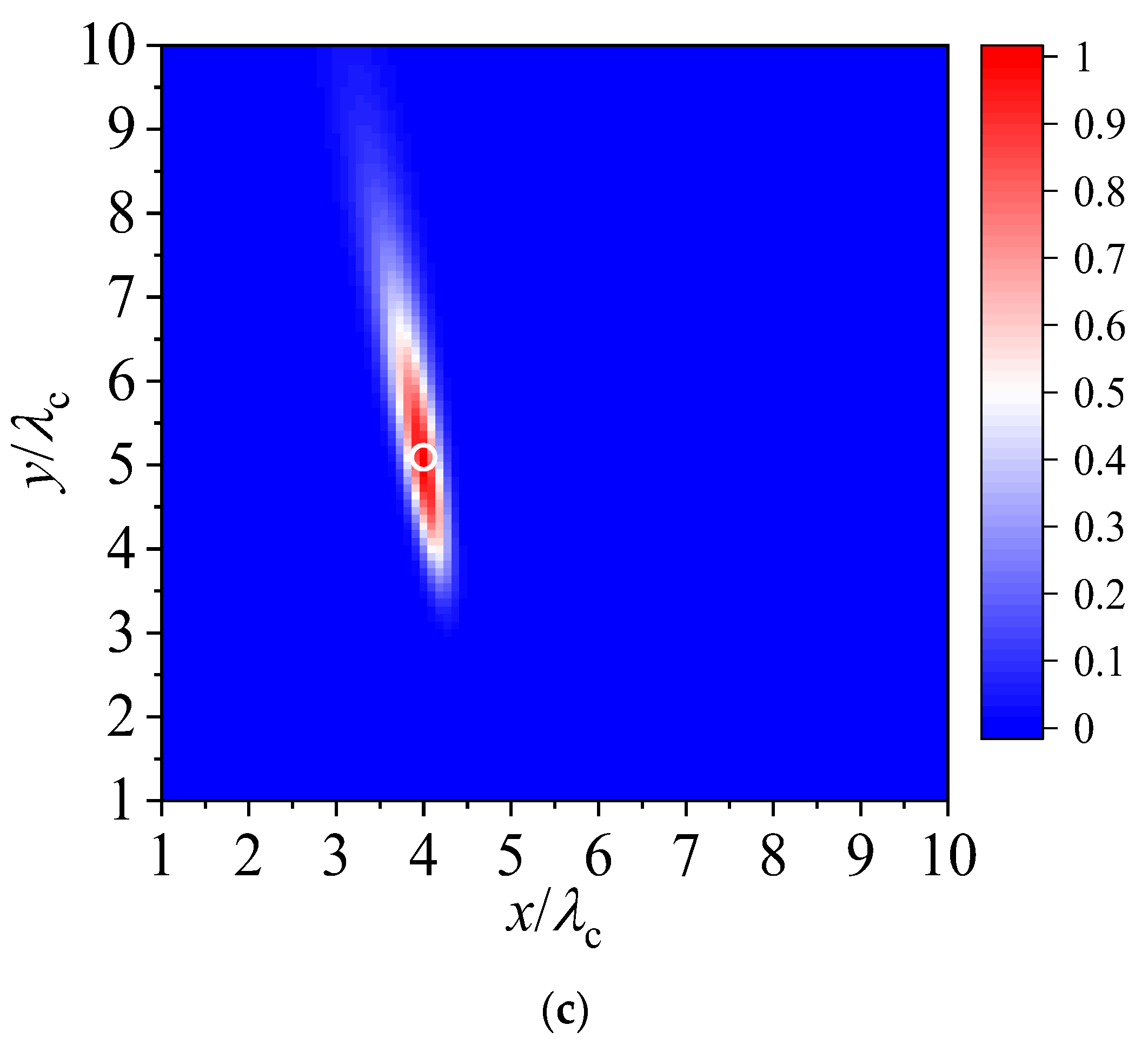
4.1. Positioning a Single Isolated R-PIMS

Firstly, the performances of positioning a single isolated R-PIMS are investigated. The position of the R-PIMS is assumed to be $P=\left(4{\lambda }_{\mathrm{c}},5{\lambda }_{\mathrm{c}}\right)$. Based on the TRO decomposition, the normalized distribution of eigenvalues of these DORT-based methods to the positioning of the R-PIMS, located at $P=\left(4{\lambda }_{\mathrm{c}},5{\lambda }_{\mathrm{c}}\right)$ at the central frequency ${\omega }_{\mathrm{c}},$ is firstly observed in Figure 2.

As shown in Figure 2, there is only one relatively larger eigenvalue when the SNR is increased to over 0 dB, which corresponds exactly to the single R-PIM located in the imaging region. With the increased SNR, the eigenvalues for the antenna element index $l\ge 2$ are approaching zero, and these eigenvectors corresponding to the eigenvalues are spanned to the noise subspace in TR-MUSIC. With that, the SNR is decreased to −10 dB, the ratio between the second largest eigenvalue and the greatest eigenvalue approaches 0.7, and the ratios of the others are also overlarge. This indicates the there is a fuzzification for confirming which eigenvalue corresponds to the R-PIMS. Moreover, with the gradual increase in the SNR, there are $M$ greatly large eigenvalue and $L-M$ extra-small eigenvalues. For positioning a single isolated R-PIMS, there are eventually one non-zero eigenvalue and ten zero eigenvalues.

Figure 3a–c shows the pseudo-spectrum images obtained by CF-DORT, TD-DORT and C-DORT, respectively. In these figures, the white circle is the real location of R-PIMS. It can be observed from these figures that the single isolated R-PIMS is accurately positioned with the maximum pseudo-spectrum at the position $\left(4{\lambda }_{\mathrm{c}},5{\lambda }_{\mathrm{c}}\right)$. The positioning image in Figure 3a illustrates the powerful pseudo-spectrum beam directed at the position of R-PIM so that the location information can be obtained in the beam. However, it is noted that there are many pseudo-spectrum extensions in addition to the x axis and y axis. Moreover, some pseudo-spectrum side lobes also exposed in the positioning image will have a bad effect on the positioning of the R-PIMS. For a comparison, the TD-DORT is also adopted to further implement R-PIMS positioning. With more frequency of participation than in CF-DORT, the pseudo-spectrum expansions and side lobes are depressed and reduced in Figure 3b. The directional pseudo-spectrum beam in Figure 3a is concentrated to form a focusing pseudo-spectrum light-spot in Figure 3b.

In our method, it can be found that the pseudo-spectrum peak at the position of R-PIMS is relatively sharp compared to those in the CF-DORT and TD-DORT in Figure 3c. Additionally, the positioning image shows the sinking pseudo-spectrum in the others’ positions, with approximately zero pseudo-spectrum by cascade process. Additionally, the pseudo-spectrum extensions and the x axis are greatly suppressed by normalization and multiplying the pseudo-spectrum for each sampled frequency. In addition to the y axis, the pseudo-spectrum extensions are little wider than those in TD-DORT but are quite reduced for CF-DORT. This is a consequence of the fact that the accurate poisoning of the R-PIMS was obtained in C-DORT.

To further compare the imaging performances of CF-DORT, TD-DORT and C-DORT, Figure 4a,b display the cross-range and range positioning resolutions for these methods, respectively. In Figure 4a, it can be observed that C-DORT has the sharpest pseudo-spectrum peak. This is because the cascading process for the spectra at each sampled frequency focuses the high pseudo-spectrum to form pointed peak at the position of the R-PIMS and causes the pseudo-spectrum at the others’ positions plunge to approximately zero. Due to the sufficient number of array elements placed at the x axis, in comparison with the single R-PIMS to be positioned, the pseudo-spectrum peak trends for CF-DORT and TD-DORT are approximately consistent. In other words, the cross-range resolutions of the conventional CF-DORT and TD-DORT will not be improved by the infinitely increased number of antenna element. However, multiplying the spectra in C-DORT further enhances the cross-range resolution with the antenna array placed at the x axis. From Figure 4a, it can be seen that DORT has the most side lobes. TD-DORT and C-DORT suppress the side lobes by frequency pseudo-spectrum accumulation and multiplication, respectively.

In Figure 4b, the range resolutions of these methods are all weakened compared with the cross-range resolutions. This is mainly because the antenna array elements are all placed at the x axis so they can effectively distinguish the cross-range arranged targets. By multiplying the spectra, the pseudo-spectrum at the others’ positions is flat and suppressed so that there are no more side lobes in C-DORT. However, via spectra accumulation, TD-DORT has some little side lobes. Though the pseudo-spectrum image of CF-DORT also has no side lobes, it has a large width of the pseudo-spectrum beam along with the y axis.

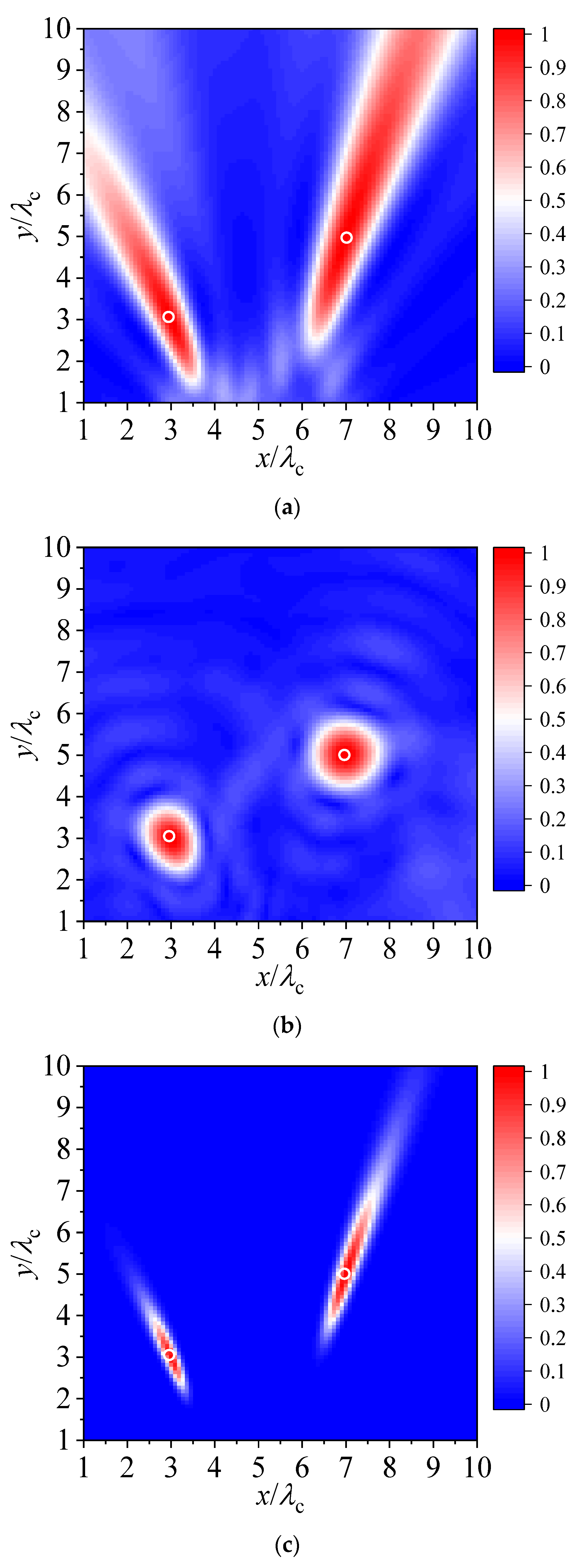
4.2. Positioning Multiple R-PIMSs

Secondly, the performances of positioning multiple R-PIMS are also investigated by simulations. Figure 5a–c shows the pseudo-spectrum images obtained by CF-DORT, TD-DORT, and C-DORT, respectively. The positions of two R-PIMS are assumed to be $P_1=\left(3{\lambda }_{\mathrm{c}},3{\lambda }_{\mathrm{c}}\right)$ and $P_2=\left(7{\lambda }_{\mathrm{c}},5{\lambda }_{\mathrm{c}}\right)$, which are shown by the white circles in these figures.

It can be observed that the CF-DORT positing image illustrates two strong pseudo-spectrum beams directing to the positions of two R-PIMSs in Figure 5a. However, the pseudo-spectrum extensions along with the x and y axis prevent the positions of targets from being obtained accurately in the positioning image. The quite wide width of the pseudo-spectrum beam, pseudo-spectrum extensions, and pseudo-spectrum side lobes in the CF-DORT method overwhelm the ability to position a mass of R-PIMS targets simultaneously and close R-PIMS targets. To improve the imaging performance, TD-DORT reduces the pseudo-spectrum extensions along in addition to the x-axis and pseudo-spectrum side lobes, as shown in Figure 5b. With the pseudo-spectrum at each sampled frequency accumulation, the different pseudo-spectrum values for the two positions are enlarged by fully sampled frequencies participating in the positioning image, and the wide width of the pseudo-spectrum beam is not effectively lessened in TD-DORT.

In our C-DORT method, as shown in Figure 5c, which is different from TD-DORT, the cascading process for the pseudo-spectrum at each sampled frequency reduces the increased number of side lobes and the cross-range width of the pseudo-spectrum around the R-PIMSs, though the number of R-PIMSs is increased to two. Moreover, C-DORT also provides a cleaner image to position more R-PIMSs because the pseudo-spectrum is suppressed to approximately zero. Consequently, C-DORT improves the imaging resolution and provides an easier way to obtain the targets’ location information and more accurate positioning imaging.

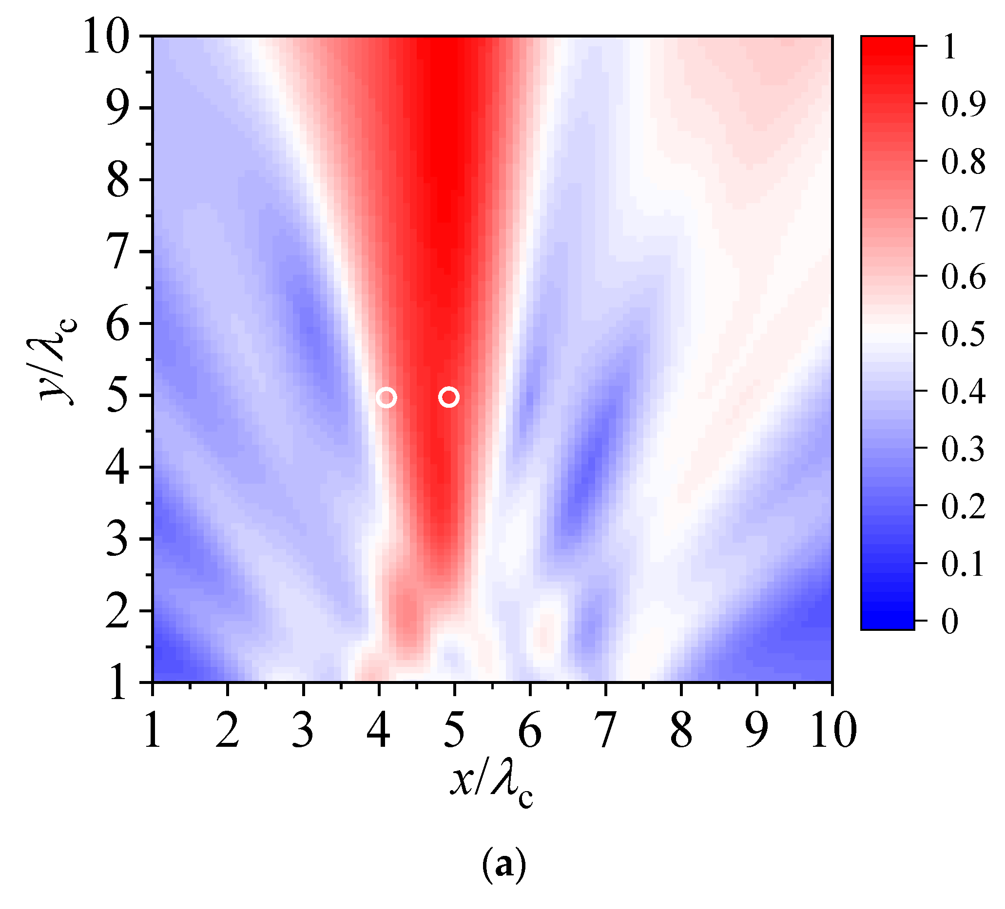
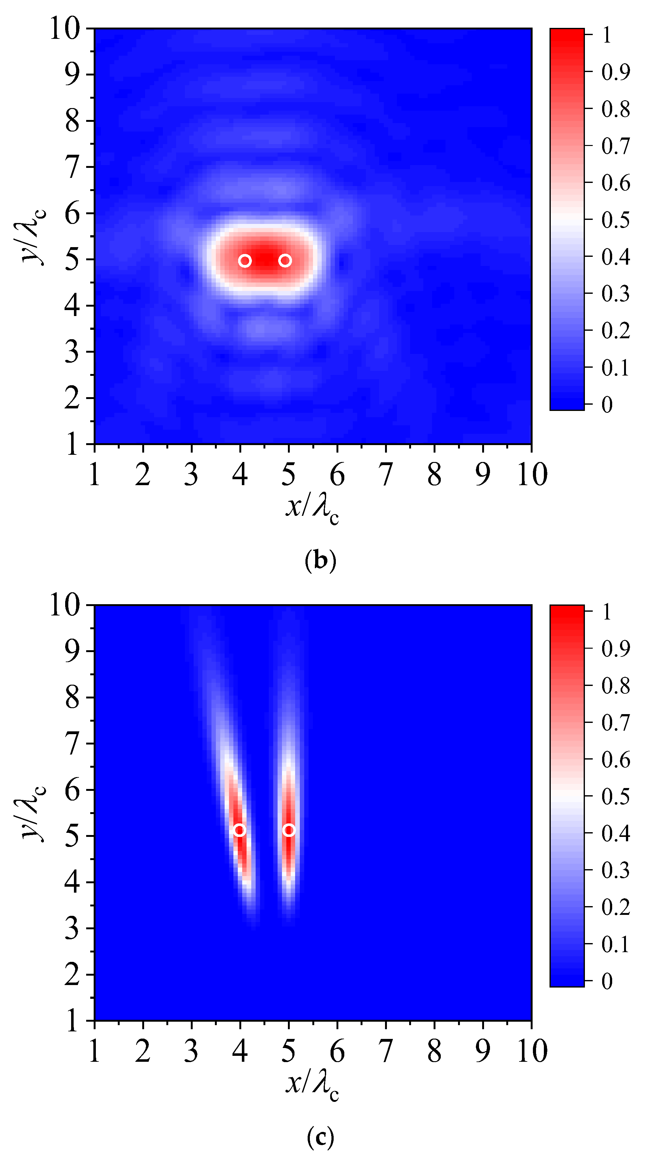
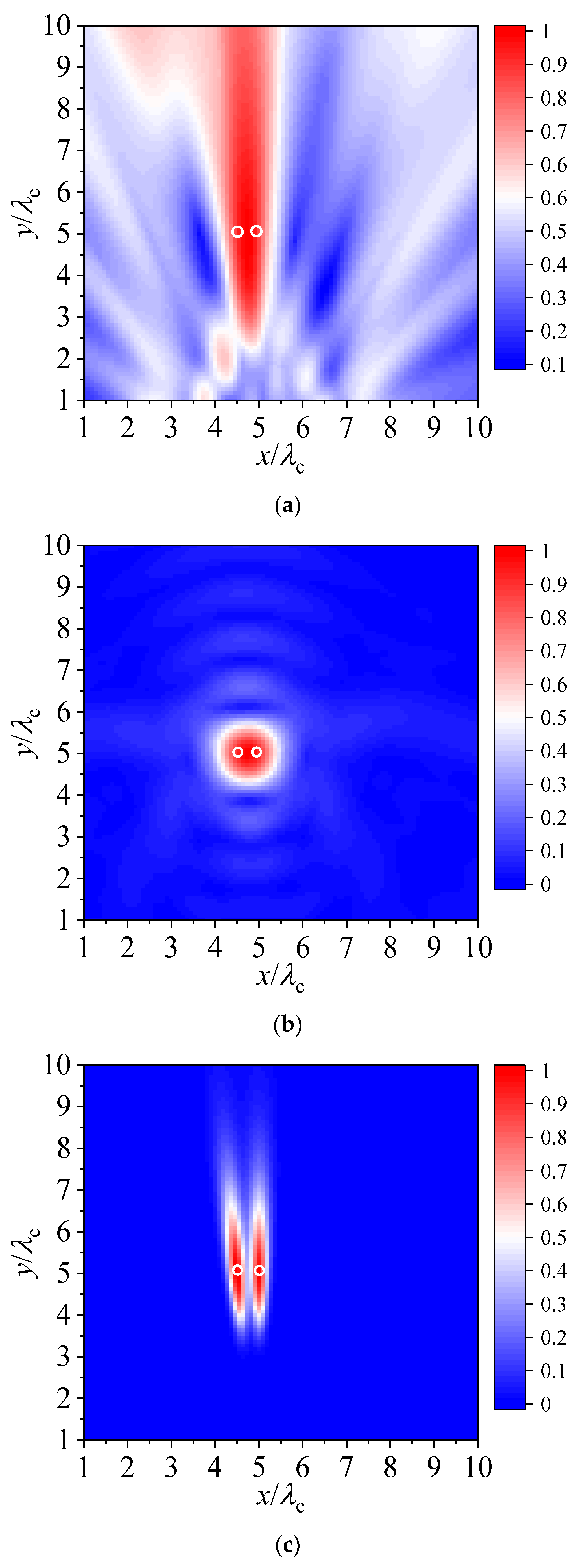
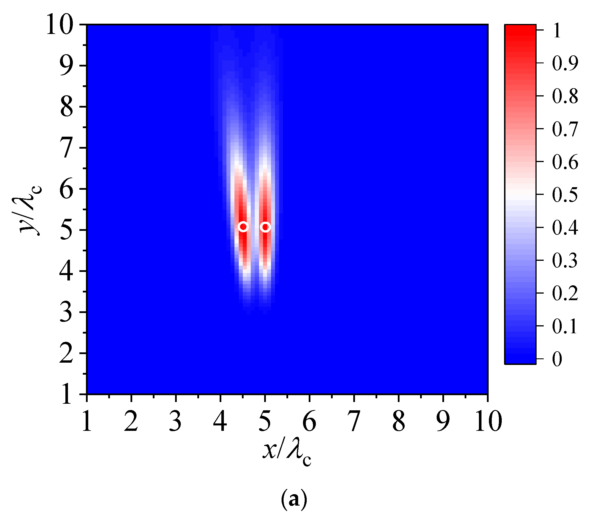
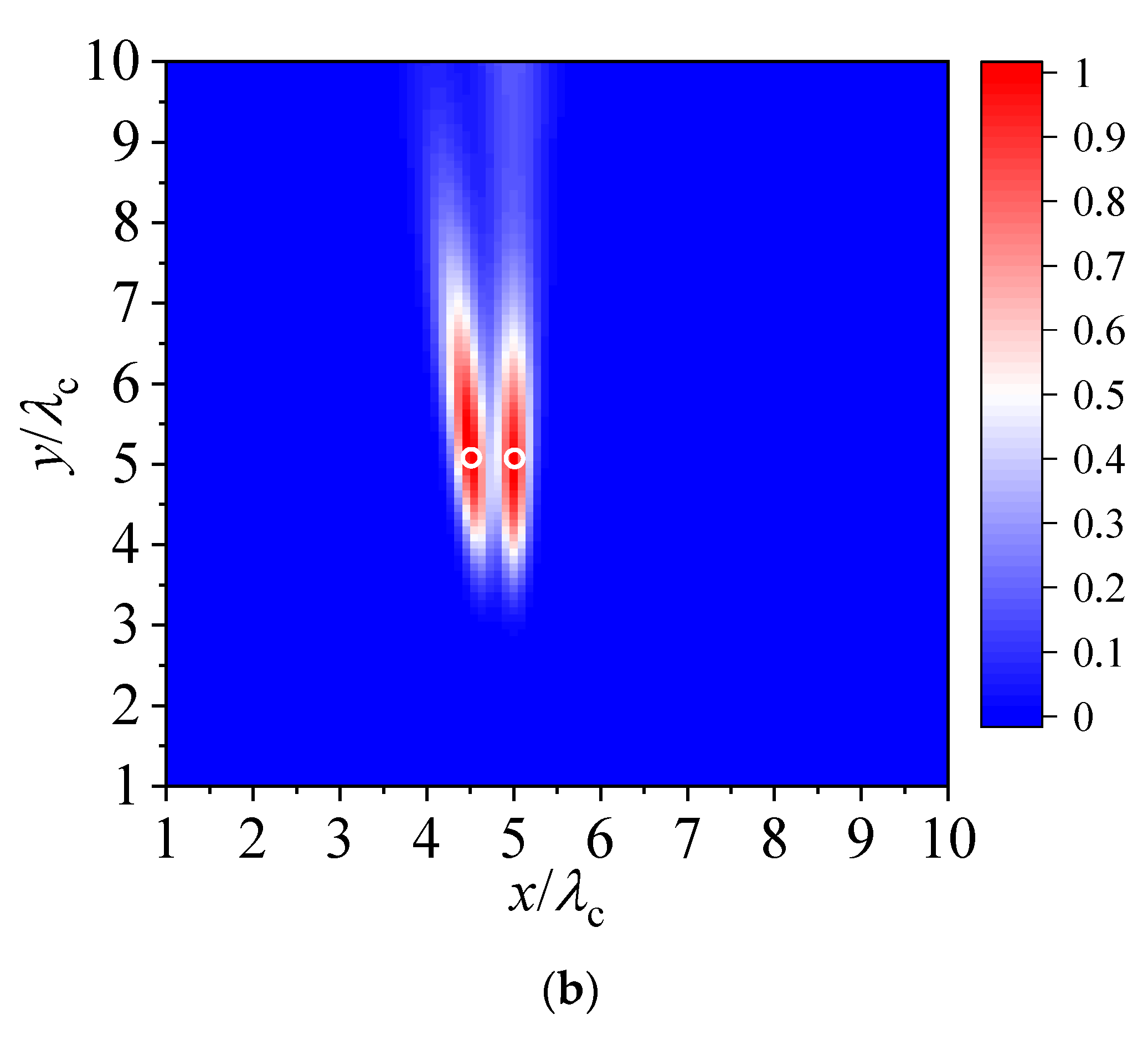
4.3. Positioning Space Adjacent R-PIMSs

To further the investigate the positioning spatial resolution performances, simulations for positioning two closely spaced R-PIMSs were carried out. The two R-PIMSs are located at $P_1=\left(5{\lambda }_{\mathrm{c}},5{\lambda }_{\mathrm{c}}\right)$ and $P_2=\left(4{\lambda }_{\mathrm{c}},5{\lambda }_{\mathrm{c}}\right)$ in Figure 6, while the two R-PIMSs are located at $P_1=\left(5{\lambda }_{\mathrm{c}},5{\lambda }_{\mathrm{c}}\right)$ and $P_2=\left(4.5{\lambda }_{\mathrm{c}},5{\lambda }_{\mathrm{c}}\right)$ in Figure 7. In these figures, the white circles are the real positions of R-PIMSs.

As shown in Figure 6a, there is only one directional pseudo-spectrum beam in the CF-DORT positioning image. This is because the cross-range width of the directional pseudo-spectrum beams for two R-PIMSs are wide so that the two pseudo-spectrum beams at two closed positions overlap to form a pseudo-spectrum beam. Figure 6b shows the positioning image of TD-DORT in positioning two closely spaced R-PIMSs. Though it can be observed that two unobvious light-spots exist, the pseudo-spectrum for the positions of the two R-PIMSs are also superposed onto each other to form a higher pseudo-spectrum peak.

From the figures in Figure 6a,b, CF-DORT and TD-DORT cannot absolutely distinguish such closely spaced targets. However, in Figure 6c, there are obviously two pseudo-spectrum peaks at the $P_1$ and $P_2$ positions, and two R-PIMSs are effectively distinguished by C-DORT. In addition to the x axis, the imaging for each R-PIMS is individual, and the pseudo-spectrum between these R-PIMSs is decreased to approximately zero. Furthermore, with a closer space between two R-PIMs at a distance of $0.5{\lambda }_{\mathrm{c}}$, which is the diffraction limit, Figure 7a,b provides a fully overlapped pseudo-spectrum beam and light-spot, respectively. However, in Figure 7c, with the cascade process in C-DORT, the two $0.5{\lambda }_{\mathrm{c}}$ closely spaced R-PIMSs are distinguished, firmly verifying the improved resolution performance.

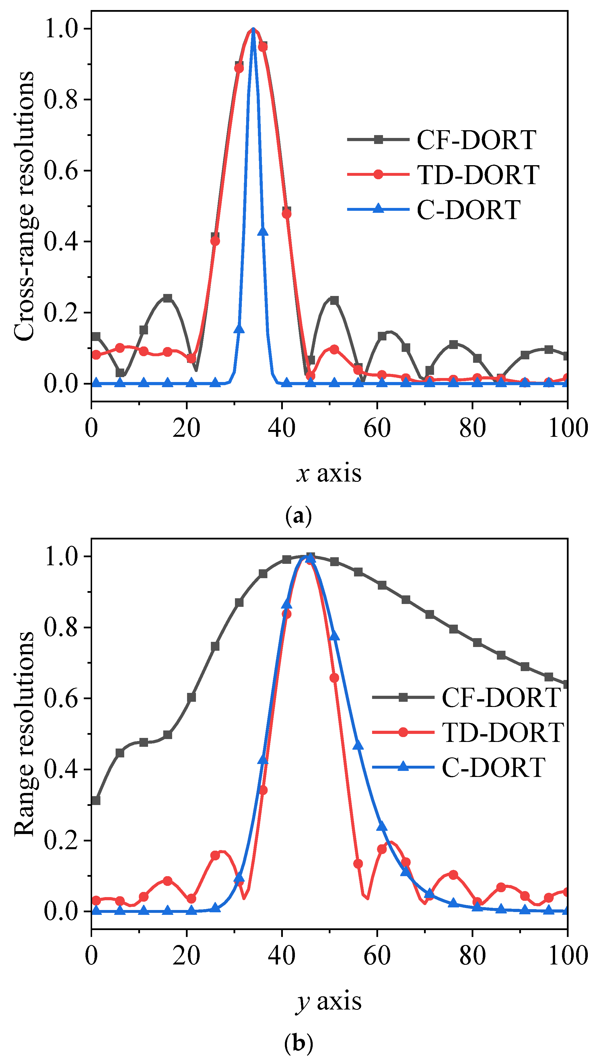
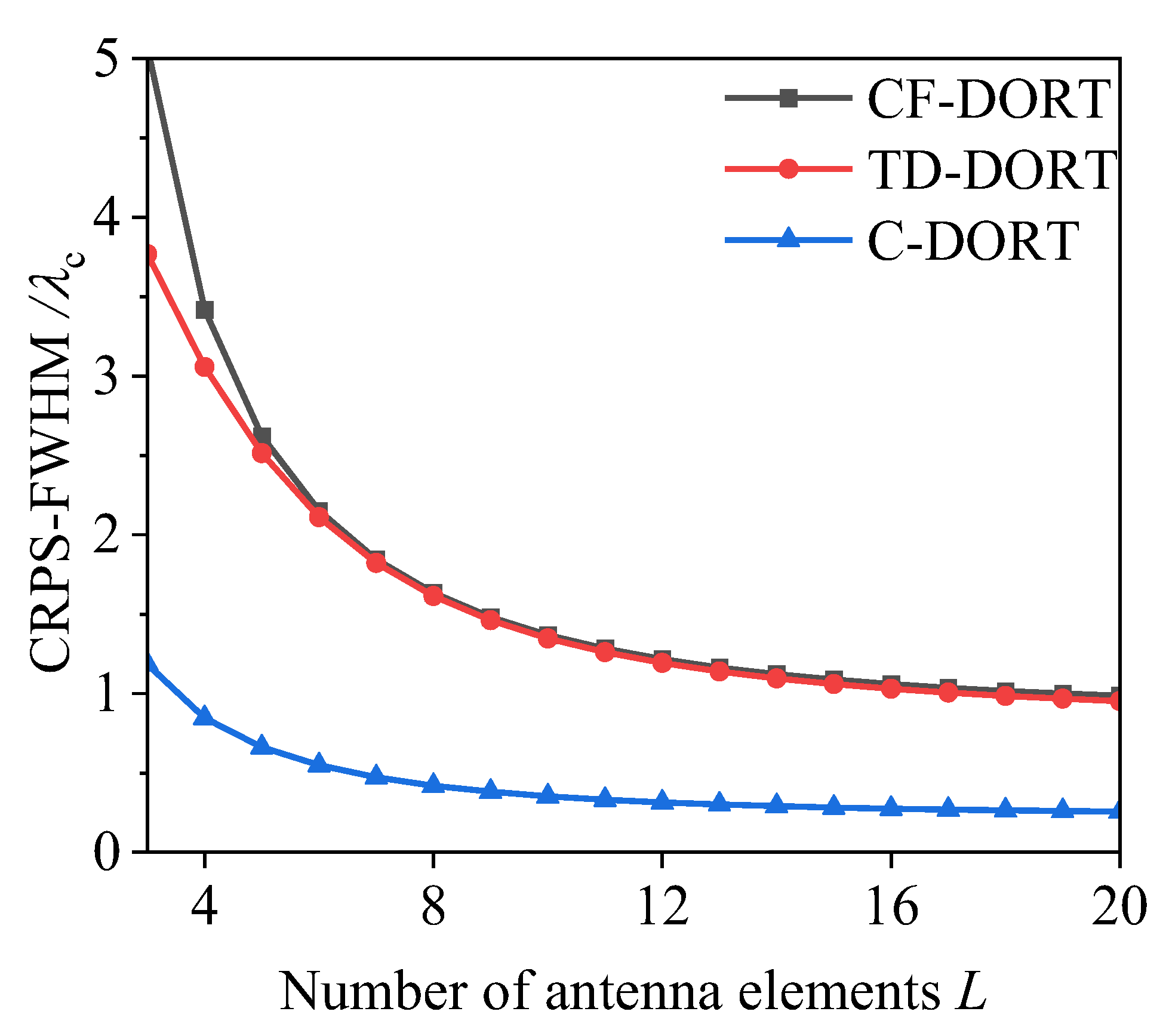
4.4. Cross-Range Pseudo-Spectrum Width

To further analyze the positioning resolution for positioning the R-PIMS, the investigation of the cross-range pseudo-spectrum full width at half maxima (CRPS-FWHM) is presented. The CRPS-FWHM in the positioning image denotes the spectra width of the pseudo-spectrum at the positions of the half-maximum pseudo-spectrum peak [33].

Figure 8 shows the comparisons of the CRPS-FWHM values with the total number $L$ of antenna elements in a noiseless space. As shown in this figure, the CRPS-FWHMs of CF-DORT and TD-DORT are larger than that of C-DORT. As previously mentioned, this is because the cascade process for each sampled pseudo-spectrum suppresses the non-R-PIMS positions. The CRPS-FWHM at the position of the R-PIMS is also reduced in CF-DORT. Hence, the cross-range resolution can be improved. When the number of antenna elements is increased to 20, the curves of the CRPS-FWHMs tend to be flat, and the cross-range CRPS-FWHMs of C-DORT and TD-DORT approach $0.25{\lambda }_{\mathrm{c}}$ and ${\lambda }_{\mathrm{c}}$, respectively. This implies that C-DORT has an ability to realize the supper resolution for closely spaced positions at a distance of less than $0.5{\lambda }_{\mathrm{c}}$. Moreover, for fewer antenna elements, the CRPS-FWHM of CF-DORT is slightly wider than that of TD-DORT; the main reason for this is that the number of antenna elements is too small to form a narrow pseudo-spectrum beam to the position of the R-PIMS.

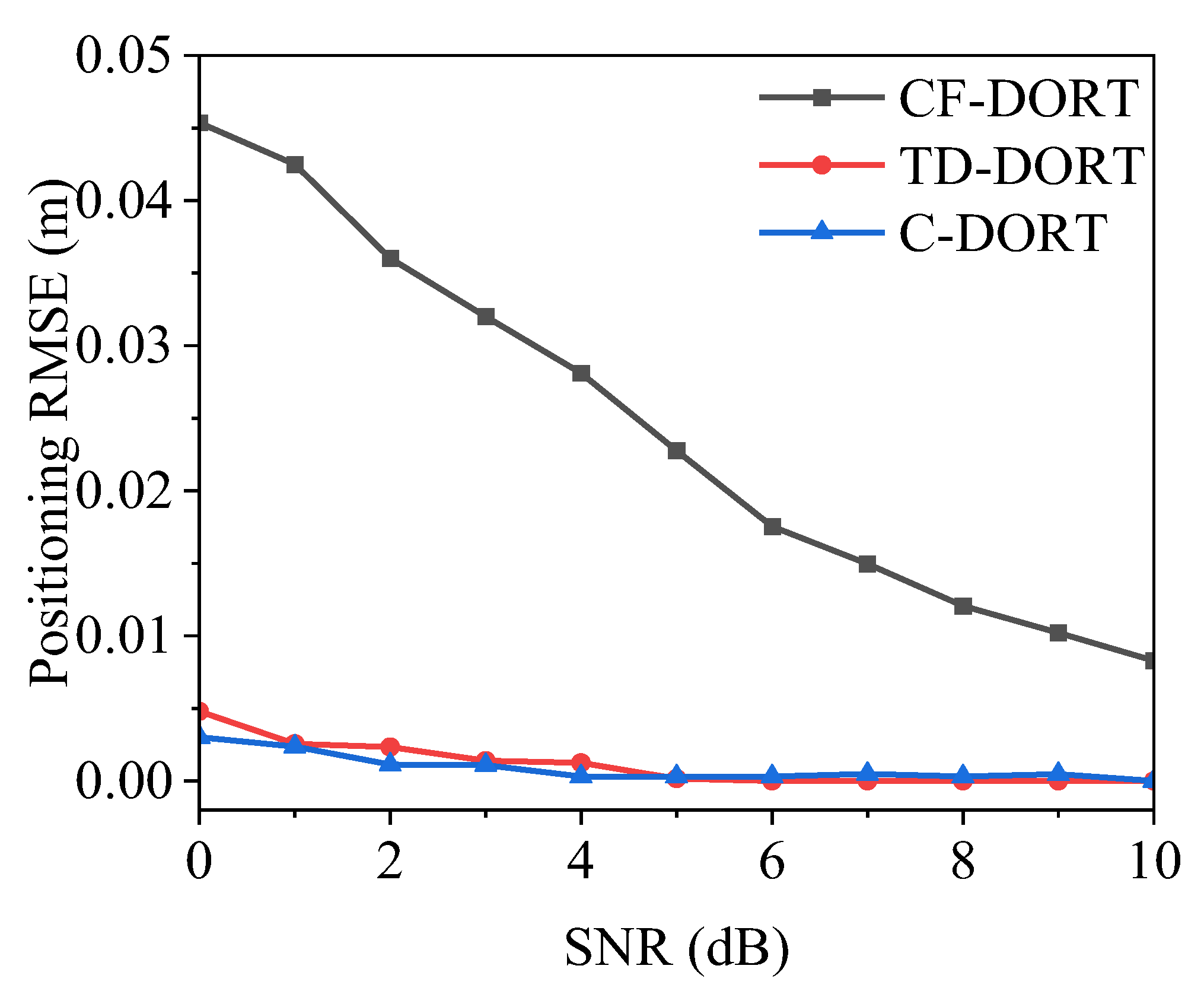
4.5. Positioning Accuracy

Additionally, the positioning accuracy has been demonstrated by analyzing the positioning error. The root mean square estimation (RMSE) and Monte Carlo method were united and adopted to analyze the R-PIMS positioning error. The positioning RMSE can be written by

$$RMSE=\sqrt{\frac{1}{Q}{\displaystyle \sum }_{q=1}^Q\left(r_q-r_{\mathrm{R}-\mathrm{PIMS}}\right)}$$

(15)

where $Q=1000$ is the number of Monte Carlo simulations, and $r_q$ represents the positions estimated by the peaked pseudo-spectrum in these DORT-based methods.

From Figure 2, the positioning RMSE at the SNR ranging from 0 dB to 10 dB was obtained by Equation (15) to analyze the positioning error. Figure 9 displays the positioning RMSE comparison to evaluate the positioning accuracy. As the DORT-based methods have a well anti-noise performance, it can be observed that there are low orders of magnitude of the positioning RMSEs for these DORT-based methods. However, with the frequency of participation in TD-DORT and C-DORT, the positioning RMSE and positioning accuracy have been improved.

4.6. Imaging Robustness

Furthermore, the imaging robustness of C-DORT for positioning two multiple R-PIMSs spaced at a distance of $0.5{\lambda }_{\mathrm{c}}$ was analyzed. The speckle noise and Poisson noise were superposed into the SS-MDMs in Equation (5) instead of Gaussian noise. Figure 10 illustrates the plane images, considering the two types of noise for positioning the two R-PIMSs located at $P_1=\left(5{\lambda }_{\mathrm{c}},5{\lambda }_{\mathrm{c}}\right)$ and $P_2=\left(4.5{\lambda }_{\mathrm{c}},5{\lambda }_{\mathrm{c}}\right)$, respectively. As shown in Figure 10a,b, the two R-PIMSs are still distinguished by superposing the speckle noise and Poisson noise onto the SS-MDMs. From Figure 7 and Figure 10, the wider pseudo-spectrum expansions and the y axis are illustrated in Figure 10b by superposing the Poisson noise onto the SS-MDMs. This is because Poisson noises have strong randomness on the SS-MDMs, and the Gaussian white noises are in accordance with a normal distribution and are mutually independent. Speckle noises always are produced by multiplying the random data in SS-MDMs, which refer to signal data in the SS-MDMs. The case of different types of noise demonstrates C-DORT has a better ability to tolerate the Gaussian white noise and speckle noises.

5. Conclusions

In this paper, a novel high-resolution and accurate C-DORT approach is proposed for positioning R-PIMS. The multiplication operator in C-DORT that suppresses the pseudo-spectrum at the non-R-PIMSs positions contributes to distinguishing the closely spaced R-PIMSs to enhance the positioning resolution. Meanwhile, the cascade process also spotlights the pseudo-spectrum at the R-PIM positions so that the positions of the R-PIMSs can be accurately located. C-DORT achieves a good positioning accuracy, with approximately zero positioning RMSE at the SNR ranging from 0 dB to 10 dB. Moreover, the two R-PIMSs spaced at $0.5{\lambda }_{\mathrm{c}}$ are distinguished effectively, and a CRPS-FWHM of $0.25{\lambda }_{\mathrm{c}}$ is obtained in C-DORT. Based on the imaging performance, the proposed C-DORT has also great potential for locating closely spaced targets in applications such as damage imaging, soft fault detection and diagnosis, through-wall imaging, and subsurface exploration.

References

1. Cheng, K.; Qu, M.; Shi, J.; Tao, X. Design of Wideband OMT Choke Flanges for Low PIM Satellite Communication Applications. IEEE Trans. Electromagn. Compat. 2022, 64, 1105–1111. [Google Scholar] [CrossRef]
2. Treviso, F.; Trinchero, R.; Keski-Opas, P.; Kelander, I.; Canavero, F.G. Sensitivity Analysis of Passive Intermodulation Due to Electrical Contacts. IEEE Trans. Electromagn. Compat. 2022, 64, 760–769. [Google Scholar] [CrossRef]
3. Jin, Q.; Feng, Q. Passive Intermodulation Distortion in Connectors With Nonlinear Interaction in Electrical Contacts and Magnetic Materials. IEEE Trans. Microw. Theory Tech. 2021, 70, 1119–1131. [Google Scholar] [CrossRef]
4. Smacchia, D.; Soto, P.; Boria, V.E.; Guglielmi, M.; Carceller, C.; Garnica, J.R.; Galdeano, J.; Raboso, D. Advanced Compact Setups for Passive Intermodulation Measurements of Satellite Hardware. IEEE Trans. Microw. Theory Tech. 2017, 66, 700–710. [Google Scholar] [CrossRef]
5. Guo, H.; Yao, Y.; Xie, Y. Evaluation of Passive Intermodulation From Multiple Connectors With Generalized Network Method. IEEE Microw. Wirel. Components Lett. 2021, 31, 312–315. [Google Scholar] [CrossRef]
6. Yang, H.; Liu, Y.; Huang, W.; Wen, H.; Zhang, X.Y. Analysis of Passive Intermodulation Distortion Caused by Asymmetric Electrical Contact. IEEE Trans. Instrum. Meas. 2022, 71, 1–5. [Google Scholar] [CrossRef]
7. Bi, L.; Gao, J.; Flowers, G.T.; Xie, G.; Jin, Q. Modeling of Signal Distortion Caused by Passive Intermodulation and Cross Modulation in Coaxial Connectors. IEEE Trans. Components, Packag. Manuf. Technol. 2020, 11, 284–293. [Google Scholar] [CrossRef]
8. Christianson, A.J.; Henrie, J.J.; Chappell, W.J. Higher order intermodulation product measurement of passive compo-nents. IEEE Trans. Microw. Theory Tech. 2008, 56, 1729–1736. [Google Scholar] [CrossRef]
9. Zhu, C.; Chen, Z.; Zhang, B.; Wang, X.; Cui, W.; Li, Y.; Zhu, Z.; Li, X.; Wang, J.; Wu, S.; et al. Testing of Passive Intermodulation Based on an Ultrawideband Dual-Carrier Nulling. IEEE Trans. Microw. Theory Tech. 2022, 70, 4017–4025. [Google Scholar] [CrossRef]
10. Xanthos, L.; Yavuz, M.; Himeno, R.; Yokota, H.; Costen, F. Resolution Enhancement of UWB Time-Reversal Microwave Imaging in Dispersive Environments. IEEE Trans. Comput. Imaging 2021, 7, 925–934. [Google Scholar] [CrossRef]
11. Haghpanah, M.; Kashani, Z.G.; Param, A.K. Breast Cancer Detection by Time-Reversal Imaging Using Ultra-Wideband Modified Circular Patch Antenna Array. In Proceedings of the 2022 30th International Conference on Electrical Engineering (ICEE), Tehran, Iran, 17–19 May 2022; pp. 42–48. [Google Scholar] [CrossRef]
12. Mukherjee, S.; Mays, R.O.; Tringe, J.W. A Microwave Time-reversal Algorithm for Imaging Extended Defects in Dielectric Composites. IEEE Trans. Comput. Imaging 2021, 7, 1215–1227. [Google Scholar] [CrossRef]
13. Wu, B.; Narciandi, G.A.; Laviada, J. Multilayered circular dielectric structure SAR imaging using time-reversal compressed sensing algorithms based on nonuniform measurement. IEEE Antennas Wirel. Propag. Lett. 2020, 19, 1491–1495. [Google Scholar] [CrossRef]
14. Li, M.; Xi, X.; Song, Z.; Liu, G. Multitarget Time-Reversal Radar Imaging Method Based on High-Resolution Hyperbolic Radon Transform. IEEE Geosci. Remote Sens. Lett. 2021, 19, 1–5. [Google Scholar] [CrossRef]
15. de Castro, B.A.; Baptista, F.G.; Ardila-Rey, J.A.; Ciampa, F. Baseline-free damage imaging algorithm using spatial frequency domain virtual time-reversal. IEEE Trans. Ind. Inform. 2022, 18, 5043–5054. [Google Scholar] [CrossRef]
16. Li, Y.; Li, M.; Pan, W.; Feng, D.; Yang, D. Sub-wavelength focusing for low-frequency sound sources using an iterative time-reversal method. Meas. Sci. Technol. 2022, 33, 125402. [Google Scholar] [CrossRef]
17. Yavuz, M.E.; Teixeira, F.L. Space–Frequency Ultrawideband Time-Reversal Imaging. IEEE Trans. Geosci. Remote Sens. 2008, 46, 1115–1124. [Google Scholar] [CrossRef]
18. Yavuz, M.E.; Teixeira, F.L. On the Sensitivity of Time-Reversal Imaging Techniques to Model Perturbations. IEEE Trans. Antennas Propag. 2008, 56, 834–843. [Google Scholar] [CrossRef]
19. Prete, M.D.; Lenoe, G. Planar phased array antenna diagnostics by a MUSIC-based algorithm. In Proceedings of the 2022 IEEE Conference on Antenna Measurements and Applications (CAMA), Guangzhou, China, 14–17 December 2022. [Google Scholar]
20. Cheng, Z.; Xue, G.; Liang, F.; Zhao, D. Frequency-Extended-Space MUSIC for Positioning PIM Sources. In Proceedings of the 2022 IEEE International Symposium on Antennas and Propagation and USNC-URSI Radio Science Meeting (AP-S/URSI), Denver, CO, USA, 10–15 July 2022. [Google Scholar]
21. Mu, T.; Song, Y. Through wall imaging based on the space-frequency time-reversal. In Proceedings of the 2018 14th IEEE International Conference on Signal Processing (ICSP), Beijing, China, 12–16 August 2018; pp. 884–888. [Google Scholar]
22. Tao, Y.; Mu, T.; Song, Y. Time-reversal microwave imaging method based on SF-ESPRIT for breast cancer detection. In Proceedings of the 2017 3rd IEEE International Conference on Computer and Communications (ICCC), Chengdu, China, 13–16 December 2017; pp. 2094–2098. [Google Scholar] [CrossRef]
23. Sadeghi, S.; Aghdam, K.M.; Faraji-Dana, R.; Burkholder, R.J. A DORT-uniform diffraction tomography algorithm for through-the-wall im-aging. IEEE Trans. Antennas Propag. 2020, 68, 3176–3183. [Google Scholar] [CrossRef]
24. Zhang, G.; He, X.; Wang, L.; Yang, D.; Chang, K.; Duffy, A. Step Frequency TR-MUSIC for Soft Fault Detection and Location in Coaxial Cable. IEEE Trans. Instrum. Meas. 2023, 72, 1–11. [Google Scholar] [CrossRef]
25. Yavuz, M.E.; Teixeria, F.L. Full time-domain DORT for ultrawideband electromagnetic fields in dispersive, random in-homogeneous media. IEEE Trans. Antennas Propag. 2006, 54, 2305–2315. [Google Scholar] [CrossRef]
26. Cheng, C.; Liu, S.; Zhang, Y. Robust and Low-Complexity Time-Reversal Subspace Decomposition Methods for Acoustic Emission Imaging and Localization. IEEE Sens. J. 2020, 21, 3486–3496. [Google Scholar] [CrossRef]
27. Kafal, M.; Cozza, A. Multifrequency TR-MUSIC Processing to Locate Soft Faults in Cables Subject to Noise. IEEE Trans. Instrum. Meas. 2019, 69, 411–418. [Google Scholar] [CrossRef]
28. Huang, C.; Scalea, F.L. Ultrasound time-reversal imaging of extended targets using a broadband white noise constraint processor. SPIE Conf. Proceeding 2023, 12470. [Google Scholar] [CrossRef]
29. Hu, B.; Cao, X.; Zhang, L.; Song, Z. Weighted Space-Frequency Time-Reversal Imaging for Multiple Targets. IEEE Signal Process. Lett. 2019, 26, 858–862. [Google Scholar] [CrossRef]
30. Hu, B.; Song, Z.; Zhang, L. Fast and Efficient Time-Reversal Imaging Using Space-Frequency Propagator Method. IEEE Trans. Signal Process. 2020, 68, 2077–2086. [Google Scholar] [CrossRef]
31. Sadeghi, S.; Madannejad, A.; Ravanbakhsh, F.; EbrahimiZadeh, J.; Perez, M.D.; Augustine, R. A new focused hyperthermia based on space-frequency DORT. In Proceedings of the 2020 14th European Conference on Antennas and Propagation (EuCAP), Copenhagen, Denmark, 15–20 March 2020. [Google Scholar]
32. Mu, T.; Song, Y. Time-reversal imaging based on joint space–frequency and frequency–frequency data. Int. J. Microw. Wirel. Technol. 2019, 11, 207–214. [Google Scholar] [CrossRef]
33. Zhang, M.; Zhang, W.; Liang, X.; Zhao, Y.; Dai, W. Detection of fatigue crack propagation through damage characteristic FWHM using FBG sensors. Sens. Rev. 2020, 40, 665–673. [Google Scholar] [CrossRef]
Figure 1. The schematic diagrams of signal models for positioning the R-PIMSs: (a) the scattering signals excited by the first antenna and (b) the scattering signals excited by the last antenna.
Electronics 12 02104 g001
Figure 2. The normalized distribution of eigenvalues of these DORT-based methods to the positioning of the R-PIMS, located at P = ( 4 λ c , 5 λ c ) at the central frequency ω c .
Electronics 12 02104 g002
Figure 3. The positioning plane images for positioning a single isolated R-PIMS located at P = ( 4 λ c , 5 λ c ) : (a) CF-DORT, (b) TD-DORT, and (c) C-DORT at SNR = 10 dB.
Electronics 12 02104 g003aElectronics 12 02104 g003b
Figure 4. The (a) cross-range and (b) range resolutions for positioning a single isolated R-PIMS at the position of P = ( 4 λ c , 5 λ c ) at SNR = 10 dB.
Electronics 12 02104 g004
Figure 5. The positioning plane images for positioning two R-PIMSs located at P 1 = ( 3 λ c , 3 λ c ) and P 2 = ( 7 λ c , 5 λ c ) , respectively: (a) CF-DORT, (b) TD-DORT and (c) C-DORT at SNR=10 dB.
Electronics 12 02104 g005
Figure 6. The positioning plane images for positioning the two R-PIMSs located at P 1 = ( 5 λ c , 5 λ c ) and P 2 = ( 4 λ c , 5 λ c ) , respectively: (a) CF-DORT, (b) TD-DORT, and (c) C-DORT at SNR = 10 dB.
Electronics 12 02104 g006aElectronics 12 02104 g006b
Figure 7. The positioning plane images for positioning the two R-PIMSs located at P 1 = ( 5 λ c , 5 λ c ) and P 2 = ( 4.5 λ c , 5 λ c ) , respectively: (a) CF-DORT, (b) TD-DORT, and (c) C-DORT at SNR = 10 dB.
Electronics 12 02104 g007
Figure 8. The CRPS-FWHM variation with the total number of antenna elements, L, in noiseless space.
Electronics 12 02104 g008
Figure 9. Comparison of positioning RMSEs among CF-DORT, TD-DORT, and C-DORT methods at different SNRs.
Electronics 12 02104 g009
Figure 10. The positioning plane images with different types noise: (a) speckle noise and (b) Poisson noise.
Electronics 12 02104 g010aElectronics 12 02104 g010b
Disclaimer/Publisher’s Note: The statements, opinions and data contained in all publications are solely those of the individual author(s) and contributor(s) and not of MDPI and/or the editor(s). MDPI and/or the editor(s) disclaim responsibility for any injury to people or property resulting from any ideas, methods, instructions or products referred to in the content.