Designing Aquaculture Monitoring System Based on Data Fusion through Deep Reinforcement Learning (DRL)

Abstract

The aquaculture production sector is one of the suppliers of global food consumption needs. Countries that have a large amount of water contribute to the needs of aquaculture production, especially the freshwater fisheries sector. Indonesia is a country that has a large number of large bodies of water and is the top-five producer of aquaculture production. Technology and engineering continue to be developed to improve the quality and quantity of aquaculture production. One aspect that can be observed is how the condition of fish pond water is healthy and supports fish growth. Various studies have been conducted related to the aquaculture monitoring system, but the problem is how effective it is in terms of accuracy of the resulting output, implementation, and costs. In this research, data fusion (DF) and deep reinforcement learning (DRL) were implemented in an aquaculture monitoring system with temperature, turbidity, and pH parameters to produce valid and accurate output. The stage begins with testing sensor accuracy as part of sensor quality validation, then integrating sensors with wireless sensor networks (WSNs) so they can be accessed in real time. The implemented DF is divided into three layers: first, the signal layer consists of WSNs and their components. Second, the feature layer consists of DRL combined with deep learning (DL). Third, the decision layer determines the output of the condition of the fish pond in “normal” or “not normal” conditions. The analysis and testing of this system look at several factors, i.e., (1) the accuracy of the performance of the sensors used; (2) the performance of the models implemented; (3) the comparison of DF-DRL-based systems with rule-based algorithm systems; and (4) the cost effectiveness compared to labor costs. Of these four factors, the DF-DRL-based aquaculture monitoring system has a higher percentage value and is a low-cost alternative for an accurate aquaculture monitoring system.

1. Introduction

Indonesia is a fish-producing country which is ranked in the top five in the world. Based on data from Statistics Indonesia (BPS), it is stated that production in the aquaculture sector will reach 14 million tons in 2022 [1]. The potential for increased production from the aquaculture sector will contribute to improving the economy in Indonesia, where in 2022 Indonesia will become an exporter of fish with an achievement of 1.2 million tons [2]. The main issues in aquaculture, especially freshwater aquaculture, are temperature conditions, pH levels, dissolved oxygen levels, and turbidity levels of pond water. This influences optimal fish growth and increases the productivity of fish yields. Aquaculture technology integrated with the Internet of Things (IoT) has been developed, such as a water monitoring system [3], smart aquaculture system [4], AI IoT-based buoy system [5], temperature water control [6], and others. The IoT system being built is a multi-sensor integration that reads data from the environment and then processes it into a control application, such as a microcontroller that drives actuators [7]. From this system model, there are several weaknesses, including the resulting data that is only a trigger to carry out commands on the actuator, the information for users is less decisive, and the lack of utilization of the usability of data to make it valuable.

Data fusion is a new paradigm for integrating multi-sensor devices to produce decisive and reliable information. Data fusion is a data processing method to improve the accuracy and quality of the resulting output and reduce data redundancy [8]. The data generated by sensors in a multi-sensor system are coordinated by data fusion through a special algorithm to provide quality output [9]. Alam et al. [10] stated that the stages in data fusion consist of four stages, i.e., signal level, pixel level, feature level, and decision level. Furthermore, there are two perspectives regarding data fusion related to IoT: the first is a single-hub data fusion system where sensors interact with only one fusion system. Second is the multi-hub data fusion sensor, where the multi-sensor system interacts first with the multi-hub sensor, and then the data are transferred to the fusion system via the multi-hub sensor. Mouli [11] systematically describes the stages of data fusion, which begin with reading data from the sensor, signal processing, transferring data to the PC console, feature extraction, fusion technique, and condition analysis/diagnosis. Methods in data fusion are categorized into four categories: statistical method, mechanistic method, data-driven method (that has sub-categories of Ensemble, Fuzzy Association, and AI), assessment method, and evaluation of metrics in the analysis of the quality [12]. In aquaculture, IoT through wireless sensor networks (WSNs) integrate data fusion to maximize accuracy in estimating the temperature in aquaculture ponds and minimize data redundancy through ISOA-SELM modeling [13]. Meanwhile, Rupok et al. [14] developed a fishery early monitoring system with WSNs combined with data fusion; the method applied is the Dempster–Shafer theory (DST), which produces an accuracy of 91.1%.

Deep reinforcement learning (DRL) is the recommended method in data fusion so that it has intelligent system capabilities that can learn continuously [15]. The ability of agents in DRL to interact with the environment can support the achievement of long-term goals without external motivation or complete knowledge of the environment [16]. DRL is the development of reinforcement learning (RL) combined with deep learning, which uses a neural network that works as an approximator function and determines the output, the policy, the action, and the value. Meanwhile, RL focuses on agents who interact with the environment based on perceiving the state [17]. In the field of aquaculture, Nicolas [18] employed deep reinforcement learning in fishery management regarding decision-making by comparing several algorithms. From the results of a comparative analysis of processing times for the nine algorithms, the TD3 algorithm has demonstrated the highest performance results.

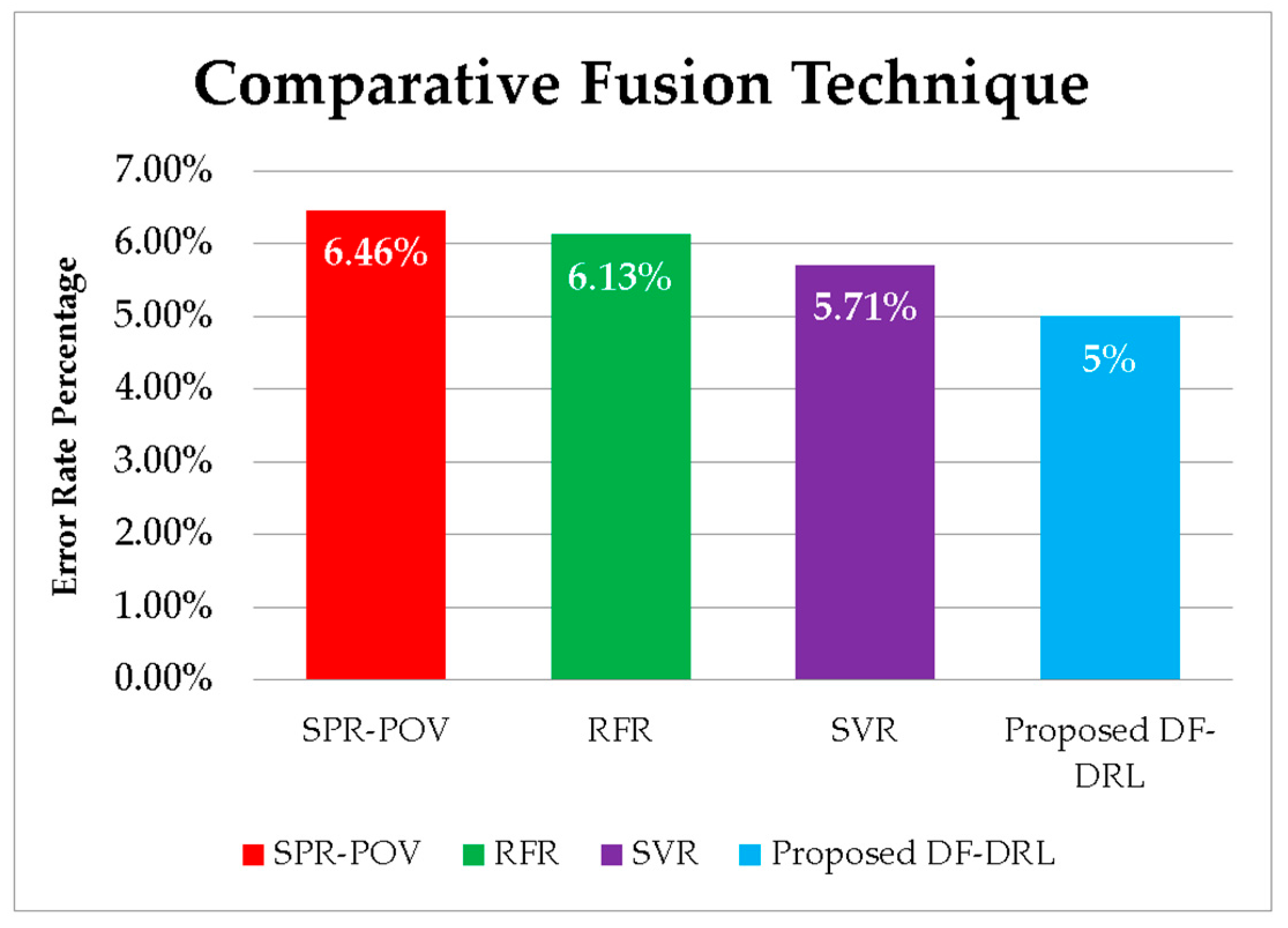
In the related work, there are several studies related to the fusion technique, including Leal-Junior et al. [19] who implement a polymer optical fiber (POF) sensor to estimate the water content of temperature-insensitive emulsions of oil–water. The surface plasmon resonance (SPR) principle is combined with POF to produce optimal output. The SPR POF output in the form of temperature is translated into a linear wavelength shift through analysis of temperature cross-sensitivity as the basis for data fusion performances. The mean error results with the fusion technique are 6.46 to 7.81%. Abadi et al. [20] employ data fusion for downscaling and evaluation of the process of evapotranspiration in water balance estimation. The data are in the form of remotely sensed data, and the fusion technique used is random forest regression (RFR) and support vector machine (SVR). Model testing was carried out by calculating the mean absolute error (MAE) value. The results of the MAE RFR and SVR tests were obtained, respectively: 6.13% and 5.71%. Manoharan et al. [21] employed a fuzzy interface algorithm in a data fusion technique for superfluous pipeline channel detection. Ultrasonic sensors are used to detect superfluous water in five scenarios with regard to the leakage point, time period of computation, period of upstream and downstream velocity, sensor performance, and cost of implementation. The final results show that the implemented data fusion model can be an alternative pattern recognition for superfluous pipeline channels in the future. Meanwhile, in this study, data fusion was implemented to integrate the data generated from the multi-sensor system, then modeling was carried out with DRL, which provides output for the user regarding the actual behavior of the object being observed in the form of a fish pond. 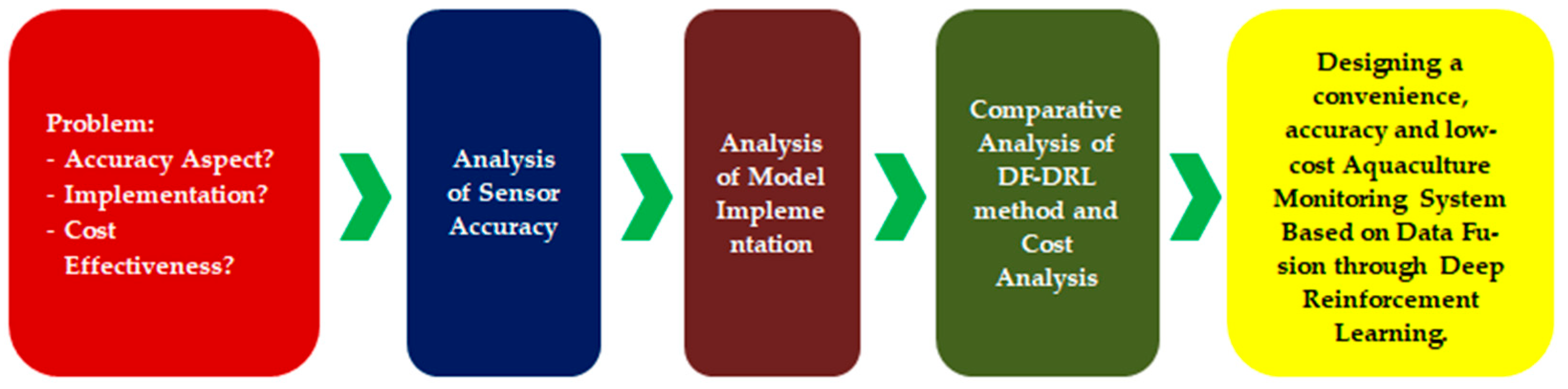Based on the experimental results and testing of the proposed system, which are discussed in more detail in Section 4, it was found that the combination data fusion-deep reinforcement (DF-DRL) had an error rate percentage of 5%, which, when compared with the three data fusion techniques, DF-DRL has a lower error rate percentage. Figure 1 shows a graph of the comparative data fusion technique:

DRL implementation employs deep learning (DL) modeling in determining the action performed by the agent, which has a major role in determining what action is performed by the system. In general, there are two main classifications of agents: model-free agents and model-based agents [22]. The model-free agent does not focus on how the model is in the environment. The learning model is based on experience, the feedback from the environment on the actions given, as well as the trial-error process. Meanwhile, model-based agents focus on how the internal model of the environment receives states or determines actions based on those states. Within the environment, various conditions or states have been determined, as well as the actions and consequences that are carried out based on these state conditions [23]. Previous research related to model-free agents, as has been done by Liu et al. [24], implements model-free agents in DRL to control the load frequency. The structure algorithm uses a deep Q network (DQN), and the final results show that the agent can solve problems by controlling the load frequency and determining the appropriate power and frequency requirements. In contrast, Sanayha and Vateekul [25] developed a model-based agent on DRL for peer-to-peer energy trading cases. Agent performance is based on an environment that has been modeled with multivariate-long short-term memory (multivariate-LSTM) with time-series data. The evaluation was carried out by forecasting the price of energy trading MAPE at 15.82%, while the predicted quantity of MAPE was 10.39%.

In this study, we employed a model-based agent where environmental conditions have been determined based on fish pond condition parameters regarding temperature, pH level, and turbidity. The agent obtains the initial conditions from the environment, the data that are integrated by the data fusion layer and then processed in the DRL framework, which becomes an action for the next stage. A detailed explanation of DRLs and agents will be discussed in detail in Section 2.4.

This paper consists of several sections: the first is the “abstract”, which explains in full a series of studies, starting with the background, the aim of the research, the methods, and the results. Second, the “introduction” section explains the background, purpose, analysis, and literature review related to the research. Third, the “system architecture design” section explains the system architecture, as well as the software and hardware of components that have been used in the research. Fourth, the “experimental method” section describes how to integrate data fusion and DRL into an integrated system to monitor aquaculture systems. The fifth “results and discussion” section describes the results based on the experiment and testing, discussing the findings of the whole experiment. The last sections are “conclusion and future work” and “references”.

2. System Architecture Design

This section describes the system architecture design, which contains an explanation of the aquaculture monitoring system, wireless sensor networks, deep fusion in the aquaculture monitoring system, deep reinforcement learning that uses deep learning as an agent, and integration of data fusion and deep reinforcement learning in the aquaculture monitoring system.

2.1. Conventional Aquaculture Monitoring System

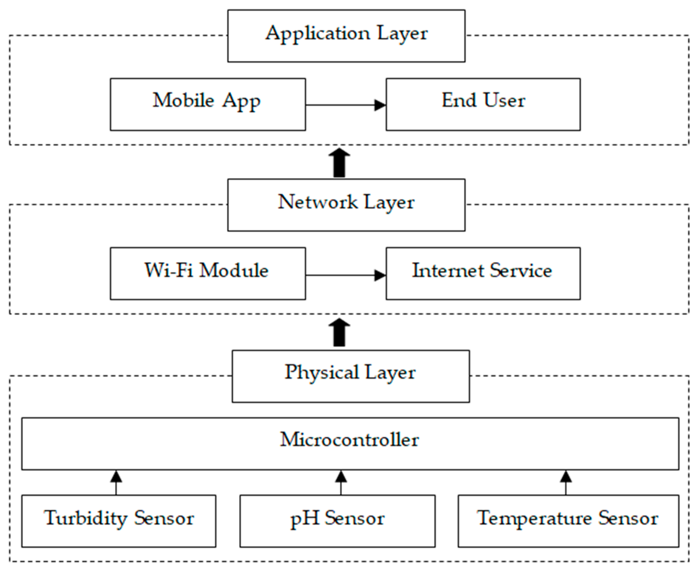
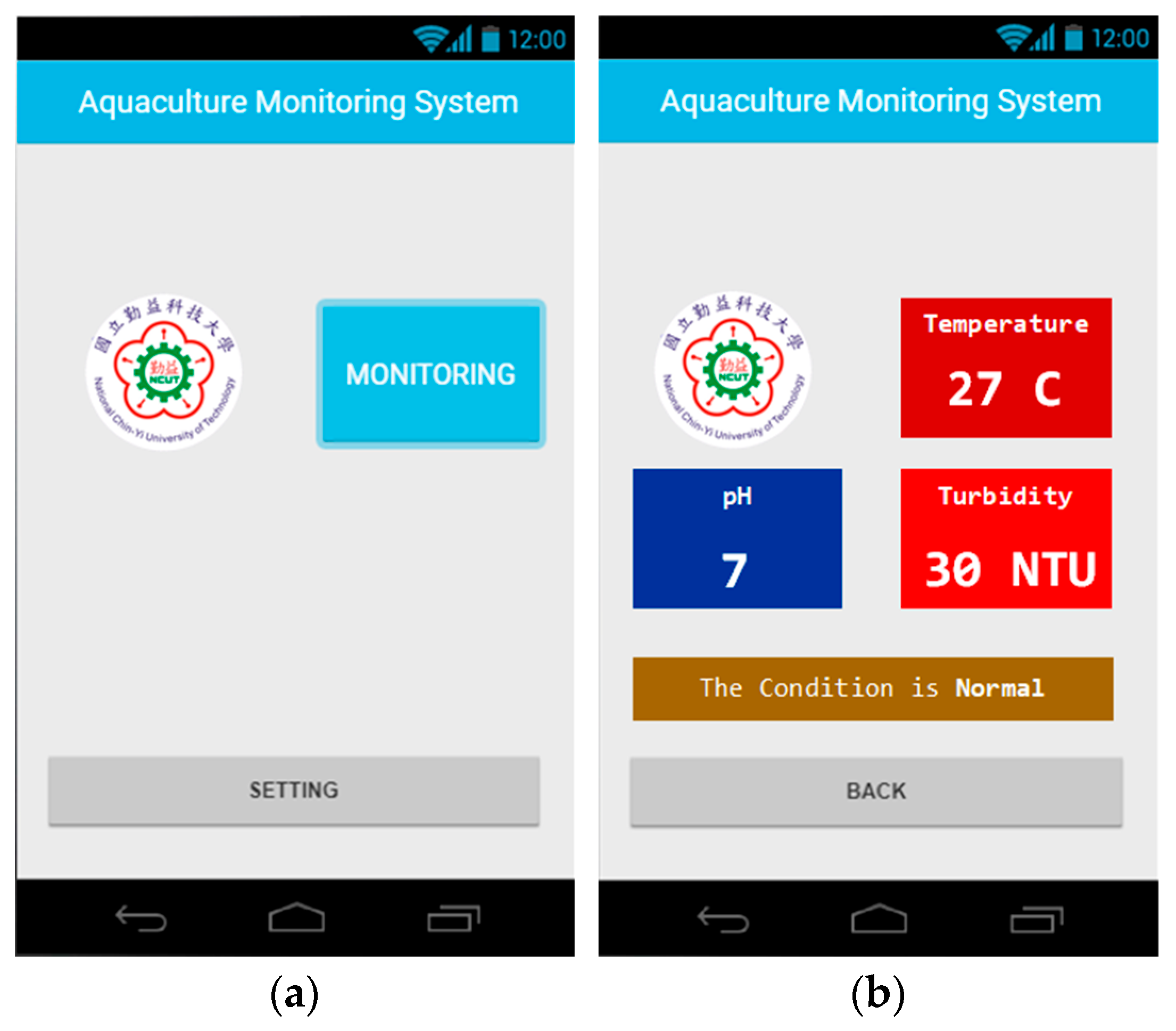
The aquaculture monitoring system in previous studies [26,27] was built with a sensor device that detects the condition of the fish pond with various parameters: temperature condition, pH level, and turbidity level. Data are read through sensors, namely the temperature sensor (type RTD PT100), pH sensor (SEN 0161), and turbidity sensor (SEN 0189), and then sent to the microcontroller connected to the Wi-Fi module. In a conventional aquaculture monitoring system, there are three layers: the physical layer, the network layer, and the application layer. The physical layer consists of sensors that are connected to a microcontroller to process data that is read by sensors from the environment. The network layer consists of Wi-Fi modules connected to internet services. The Wi-Fi module functions as an intermediary between the controller and the user via internet services. Meanwhile, the application layer is a user interface that represents the data generated by reading the device in real time from the fish pond. The applications contained in the application layer are Android-based mobile applications, which can be accessed by users anytime and anywhere. In this monitoring system, the user can only find out the current condition of the fish pond based on the parameters of temperature, pH, and turbidity. In contrast, the proposed aquaculture monitoring system not only reads the real-time condition of fish ponds but also determines whether the current condition of fish ponds is “normal” or “not normal”. Figure 2 represents the architecture of a conventional aquaculture monitoring system.

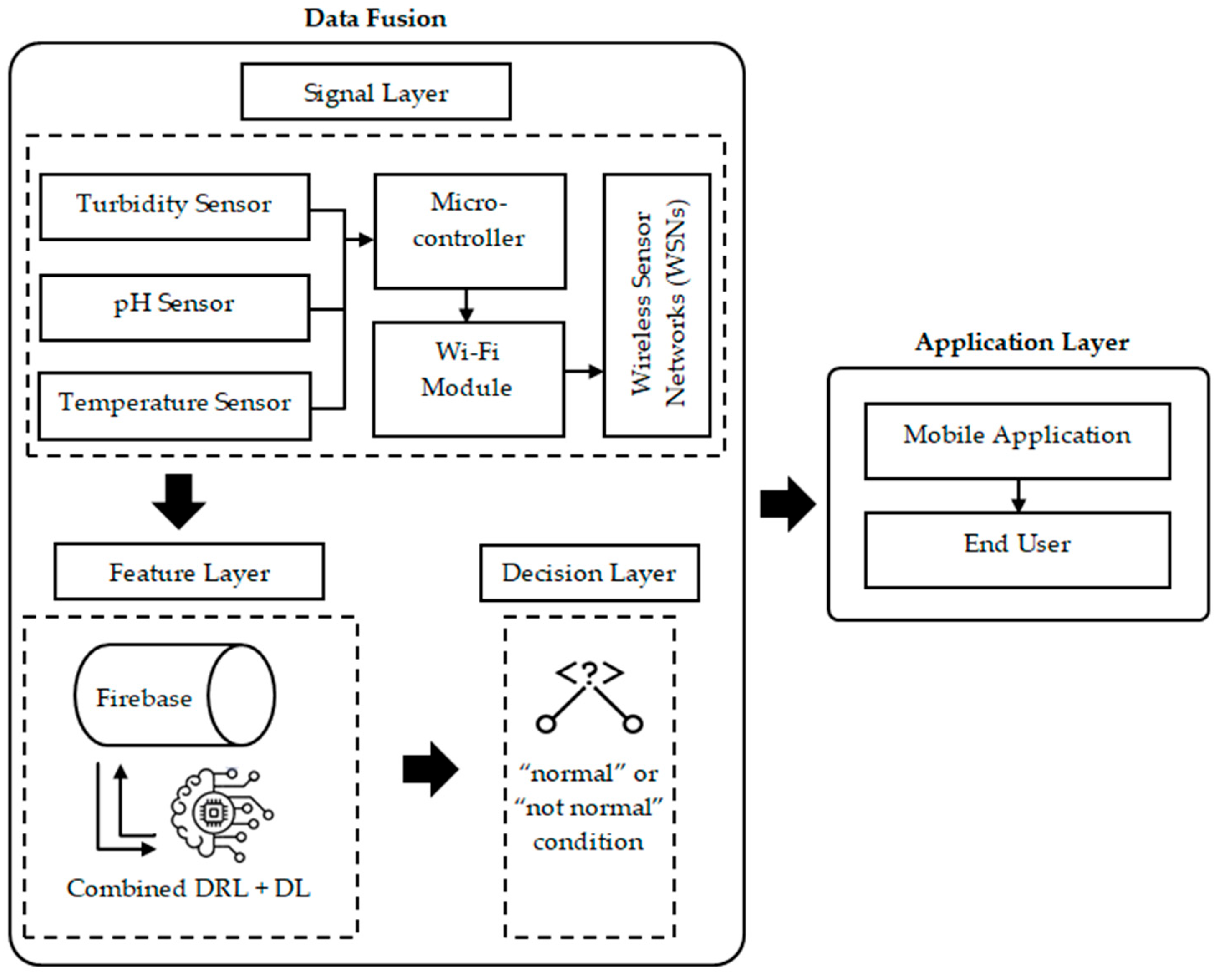
In the proposed aquaculture water monitoring system, a more complex data fusion implementation is carried out, consisting of three main layers: the signal layer, feature layer, and decision layer. The fusion technique uses a combination of DRL and DL to produce the output of the current condition of the pond, whether it is “normal” or “not normal”. The system not only reads the current conditions of the fish pond based on temperature, pH, and turbidity, but also provides the convenience for the end user to find out whether the condition of the fish pond is normal or not. Figure 3 is the proposed aquaculture monitoring system, which is discussed in detail in Section 2.6:

2.2. Wireless Sensor Networks in Aquaculture Monitoring System

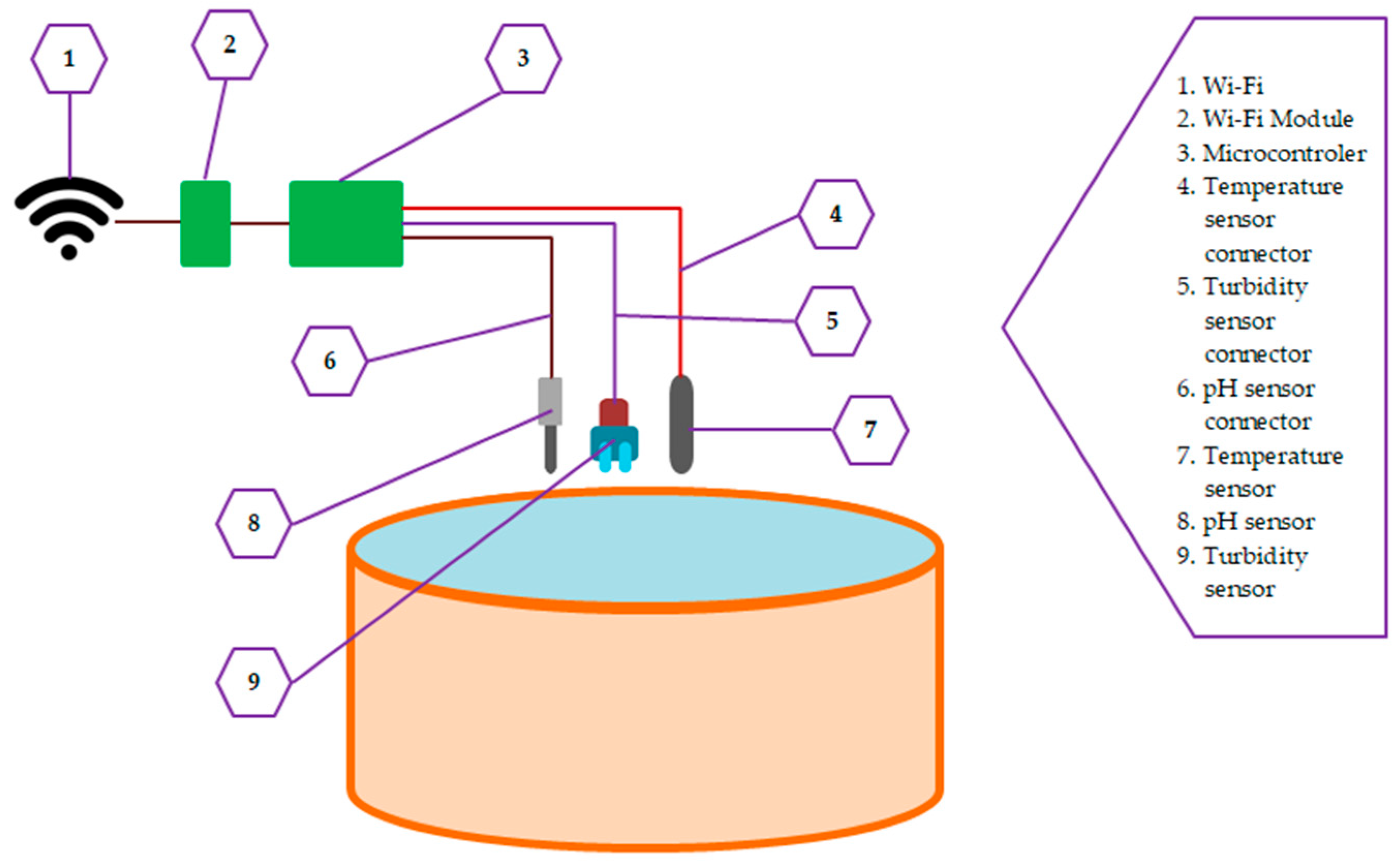
WSNs read the basic conditions of fish ponds through temperature, pH, and turbidity with integrated temperature sensor (RTD PT100), pH sensor (SEN 0161), and turbidity sensor (SEN 0189) components that are received by the ATmega328-type microcontroller provided by Arduino Uno R3, then connected to the internet and accessible by the user. The selection of sensors used in this study considers three aspects, i.e., low cost, precision, and convenience. The goal of this study is to construct a convenient, accurate, and low-cost aquaculture monitoring system based on data fusion through deep reinforcement learning. The microcontroller, as part of it, has an important role in processing data generated from sensors to become the basis for determining decision parameters.

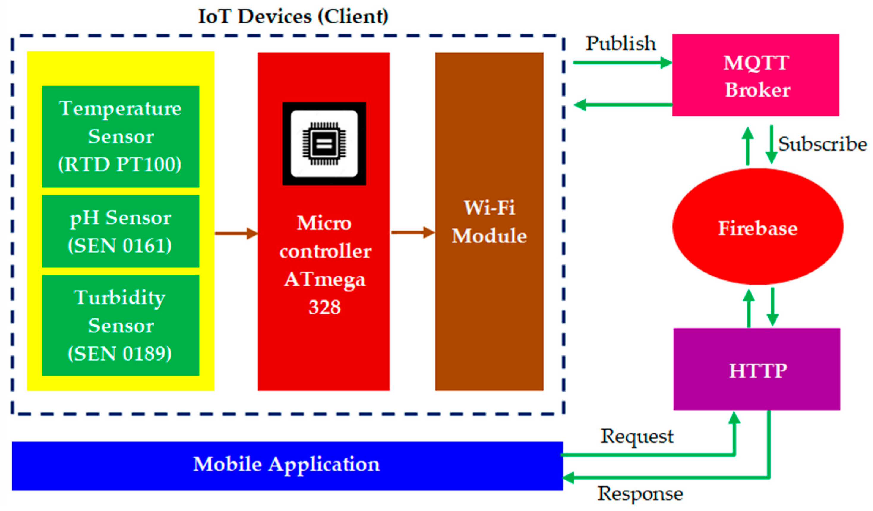
Figure 4 shows a more detailed architecture, which gives an idea of how WSNs are implemented. The data that have been processed by the microcontroller are then connected to the Wi-Fi module to be stored in the Firebase data cloud. The connection mechanism used is message queuing telemetry transport (MQTT), which connects communications between IoT machines or devices—in this case, sensors, microcontrollers, and Wi-Fi module devices—with the cloud gateway in Firebase. Furthermore, the data are stored in Firebase as real-time data on the current condition of the fish pond. MQTT works as a broker that receives data from IoT devices as a client that publishes data on the temperature, pH, and turbidity of fish ponds. MQTT is sending data to the Firebase data cloud as a subscriber of MQTT [28]. The end user or mobile applications use the Hypertext Transfer Protocol (HTTP) as a protocol that communicates data in real time on Firebase to be received by end users through Android-based mobile applications. The data communication process between the mobile application and Firebase uses “request” and “response” communication, in which the mobile application “requests” data from the system, and the system provides feedback through the “response” function by providing the latest data on fish pond conditions. The end user of the system is an Android-based application with detailed technical specifications, as referred to in Section 3.5.

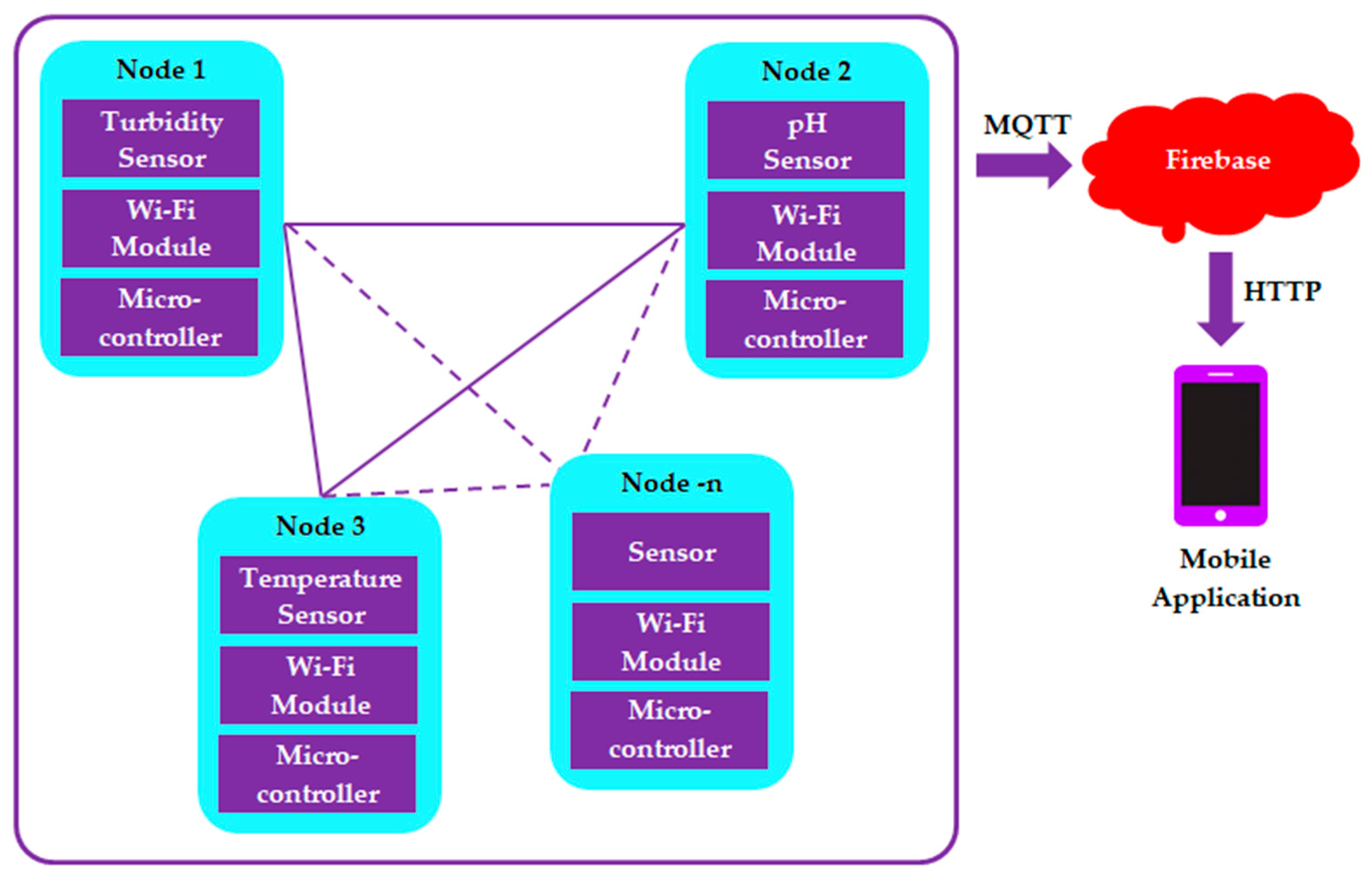
Technically, the configuration of WSNs in the aquaculture monitoring system can be seen in Figure 5, where several nodes are integrated with each other. Inside the node are a sensor, microcontroller, and Wi-Fi module. Nodes interconnect with each other to form a network called WSNs, and data are transmitted to Firebase via the MQTT protocol as the WSN’s network communication service. The Wi-Fi module acts as a data collector and also transmits data to the base station in the form of Firebase’s real-time data cloud. During data transmission between devices and Firebase, as well as mobile devices and Firebase, there are protocols used as communication media, i.e., MQTT and HTTP. Firebase acts as a storage unit that stores data read by sensors and distributes data to mobile devices.

The WSN’s network topology in this study is a mesh topology, where all nodes are interconnected or have multiple nodes. The mesh topology has the advantage in that the connected nodes complement each other’s data; for example, if the pH sensor does not work, then the data will be provided by other pH sensors connected to the WSN network. The n-th node in Figure 5 shows that as many nodes can be interconnected into this mesh topology as we need [29]. The considerations in this study using a mesh topology are the aspects of scalability, cost-effectiveness, reliability, and the effectiveness of energy.

2.3. Data Fusion in Aquaculture Monitoring System

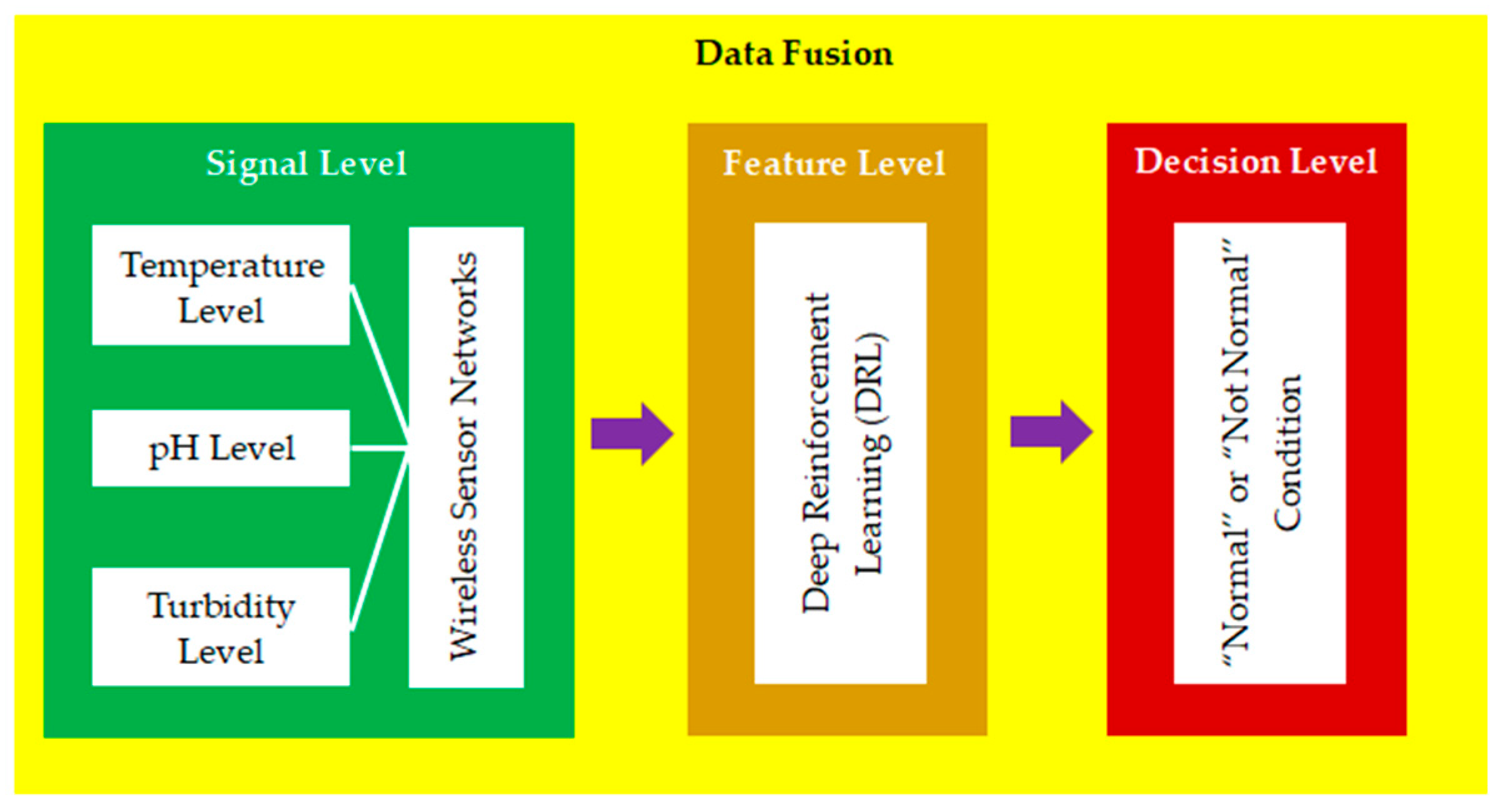
In this study, data fusion is implemented to integrate various sensors from a multi-sensor system. The system data fusion architecture is represented in Figure 6, which consists of three levels: (1) signal level; (2) feature level; (3) decision level. At the signal level, the resulting signal output based on sensor readings is integrated for use in the next layer, where the sensor reads the condition of the fish pond with the parameter’s temperature, pH, and turbidity. The raw data that are read by the sensors that are integrated with the microcontroller are then processed and transferred via the WSN as a data control for further processing, which is transmitted to the feature level. The feature level is the second process, which is the process of extracting data generated at the signal level to produce features used as parameters in making decisions or actions to be carried out by the system. A fusion technique is involved in the inferencing process in this study which uses DRL as a fusion technique for data processing. Technically, the DRL mechanism used in the fusion technique involves deep learning when the agent makes decisions. A series of neural networks is employed to produce an accurate model for determining the resulting output; detailed descriptions of DRL and DL are explained in Section 2.4 and Section 2.5. The decision level is the last in the data fusion architecture, where at this level the system issues output as a result of processing data through the data fusion process. The output generated by the aquaculture monitoring system is a notification of the condition of the fish pond in a “normal” or “not normal” condition that refers to Section 3.3. The variety of sensors used in the multi-sensor system in this study allows for a variety of complex conditions to occur, which need to be handled not only by rule-based decisions or conventional aquaculture monitoring systems, but as a whole, need to be examined from the stages of signal processing, signal information extraction, signal processing, and the output of signal processing. Therefore, the data fusion system is the choice used for this aquaculture monitoring system research.

2.4. Deep Reinforcement Learning (DRL)

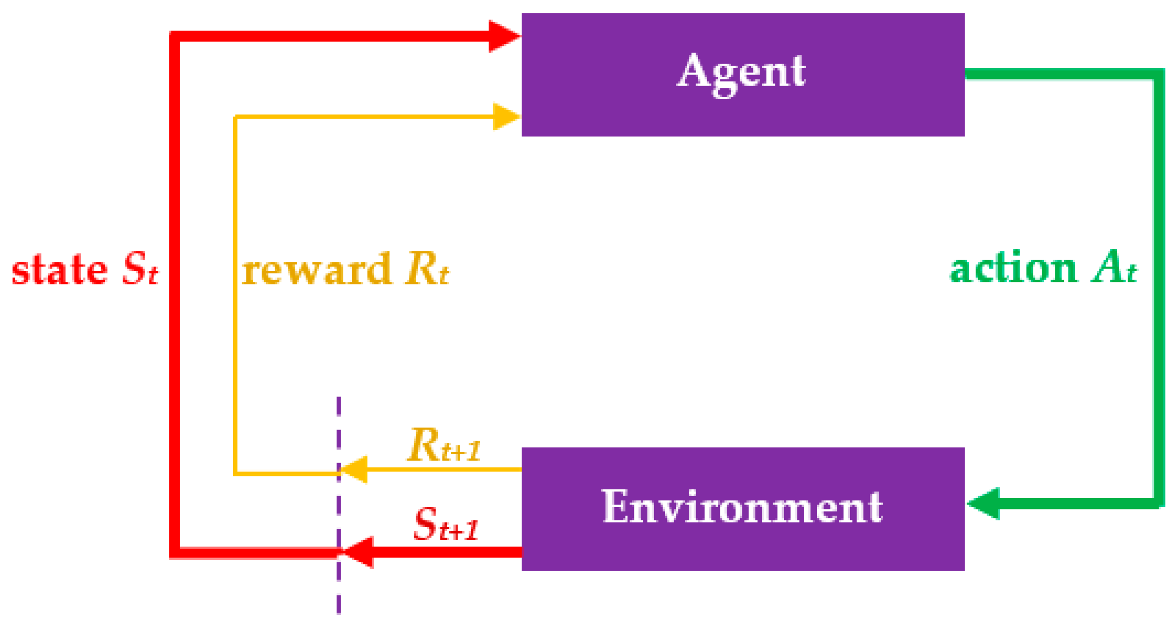
The basic concept of DRL is reinforcement learning (RL), which is part of machine learning. RL is based on the Markov decision process (MDP), which is a decision-making model in random situations represented by agents as decision-makers [30]. There are five elements in the MDP framework: agent, environment, state (S), action (A), and reward (R). The agent has a function as a decision-maker for what action will be taken by the system based on the conditions of the environment. The environment has a role in giving S to the agent so that he can make decisions in the form of A. A decided by the agent becomes input for the environment, which then becomes R for the consequences decided by the agent. Each lap time is represented by t. This process takes place continuously; the process is returned to a new state, S_(t+1), for the next decision process, and the reward is returned to the agent, R_(t+1), for the next process. If it is related between S_t, A_t, and R_t+1, it is formulated as a function f(S_t, A_t) = R_t+1, where S_t and A_t will produce a new reward, which is represented as R_t+1 on the dotted line on the left side of Figure 7, and then returns to the reward condition of the current R_t. This also applies to S_t, where it will become the new condition S_t+1 until the dotted line, and then return to S_t.

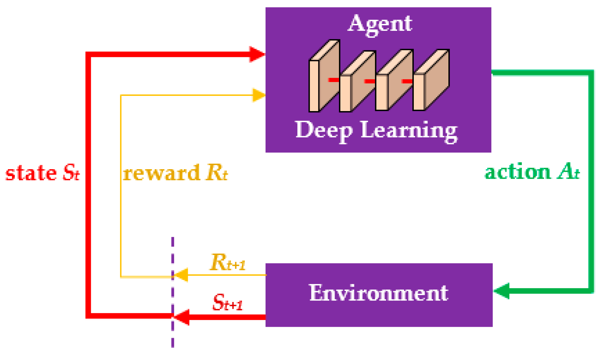
RL combined with deep learning (DL) becomes deep reinforcement learning [31]. The neural network is employed to help the agent in the decision-making process of determining the action to be performed. Figure 8 shows the extended RL combined with the DL, which becomes the DRL.

In DRL, the neural network that is used in deep learning has a function called a function approximator. DL has an important role in the DRL framework, especially in making decisions for random and complex conditions [32] and providing optimal output and rewards for the next iteration of the process. State in the context of DL in this study is the condition of the fish pond which consists of temperature conditions, pH conditions, and turbidity conditions. For example, the state temperature is 25 °C, the turbidity is 24 NTU, and the pH is 7, which are denoted as S: [7,24,25]. Then, with these conditions, the action is in the form of a declaration of the condition of the fish pool in a “normal” state, which is denoted as A: normal, which then triggers the system to give a reward (R) to become the next condition R_t+1 and S_t+1. The action determined by the agent is combined with the neural network process through the function y = f(w₁x₁ + w₂x₂ + … + w_nx_n + b) where w is the weight resulting from the model, x is the input from the neuron, and b is the bias. An activation function is implemented to produce optimal output which is represented by f. The following formulation is used in Equation (1):

Agent (St, A_t) = R_t+1 + f(w₁x₁ + w₂x₂ + w₃x₃ + … + w_nx_n + b)

(1)

As explained in the Introduction section, the agent that is built is a model-based agent, which monitors the model of its environment when it is operated. The model becomes the basis for agents to predict future actions and conditions. This model contains various states and potential actions, as well as consequences or rewards that will be obtained by agents in the DRL sequence. The selection of a model-based agent is based on environmental conditions, that is, the parameters or states contained in the aquaculture monitoring system, which consist of temperature, turbidity, and pH. Therefore, this allows the agent to make the correct and accurate decisions based on environmental conditions and the state read from the environment.

2.5. Deep Learning (DL)

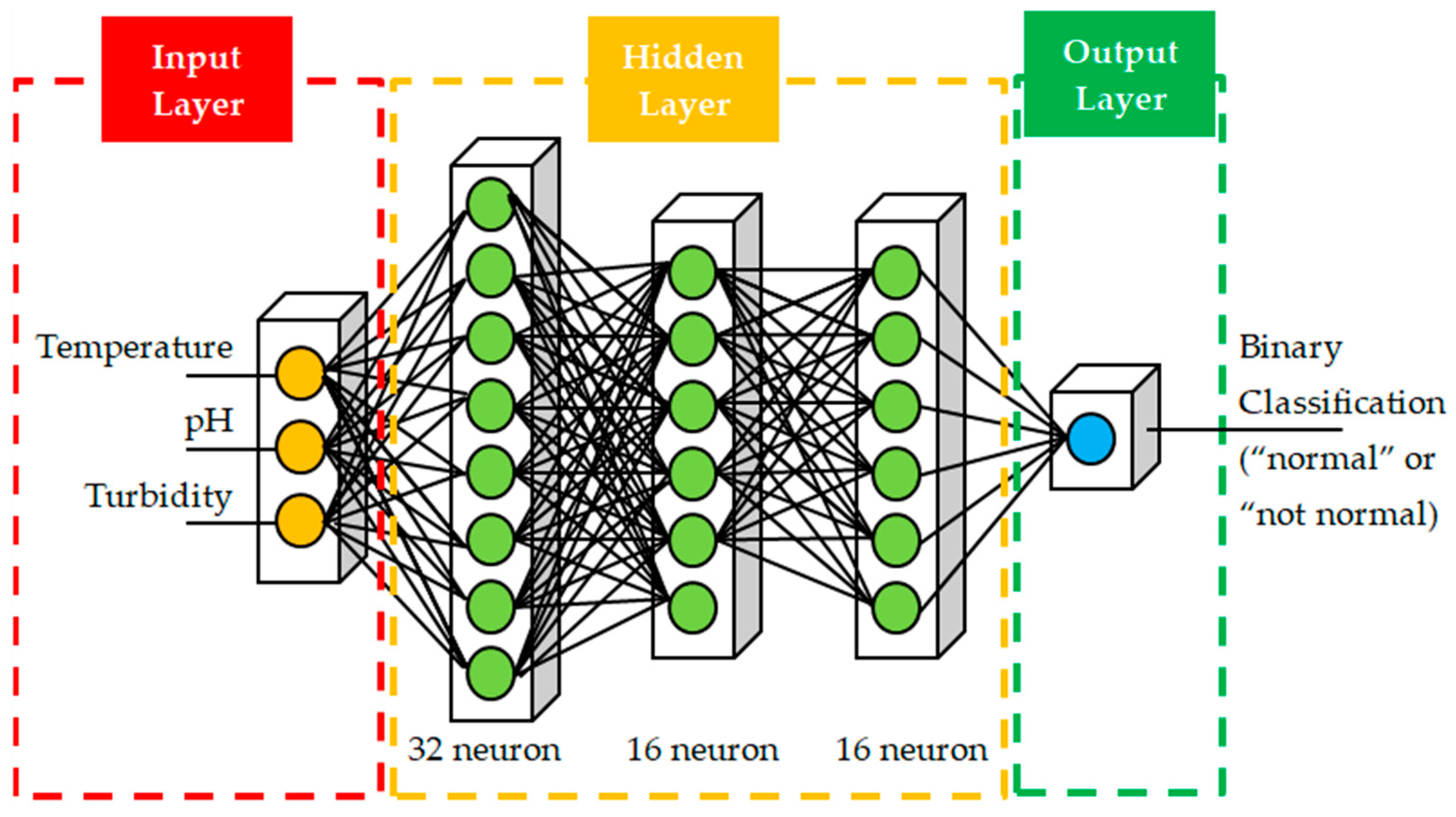
DL is a tool to sharpen the action produced by the agent, with random probability conditions [33]. In previous research, in the context of DRL, many used traditional supervised learning models such as SVM or random forest [34,35,36], thus the use of DL in this study is still relevant in the context of the updated method being implemented. The DL implementation in this study uses an artificial neural network (ANN), which is defined by five layers, consisting of one layer as the input layer, three layers as hidden layers, and one layer as the output layer. DL, together with the agent, accepts the state conditions, and then DL performs an algorithmic process to determine the probability of these conditions, where the input conditions are divided into three parts, namely temperature conditions, pH conditions, and turbidity conditions. Figure 9 represents the neural network architecture in deep learning:

In Figure 9, in which the input layer section can be seen, there are three data inputs that are the basic parameters of neurons (temperature, pH, and turbidity) to be computed in the next layer. In the hidden layer, each layer consists of 32 neurons, 16 neurons, and 16 neurons. Meanwhile, in the output layer, there is one layer in the form of binary classification 0 and 1, which represents “normal” or “not normal” fish pond water conditions. The input into each neuron is called a vector x = (x₁, x₂, x₃, ... x_n), and the output of the neuron is represented by y. In input processing, each neuron requires not only the input x but also the weight (w) that contributes to producing a strong output and provides the direction of the connection to the next neuron. To carry out x and w processing, an activation function (f) is needed so that it produces a non-linear output that will be transferred to the next neurons [37]. In the formulation Equation (2), output neurons are represented by y, which consists of f, which is an activation function that processes inputs w₁x₁, w₂x₂, w₃x₃, to w_nx_n and added by b, which is a representation of the bias [38].

y = f(w₁x₁ + w₂x₂ + w₃x₃ + … + w_nx_n + b)

(2)

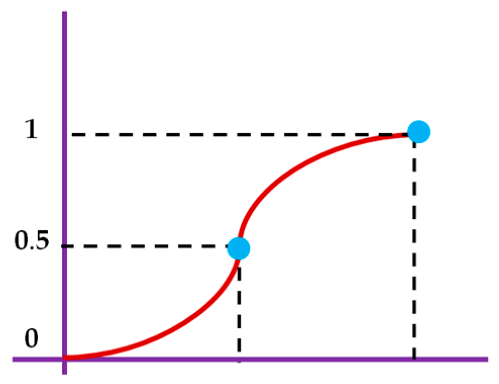
In this study, the activation function formulation used is sigmoid because it has compatibility with the resulting output in the form of binary classification in the form of 0 and 1 which represent “normal” and “not normal” output conditions. Sigmoid is denoted by the formula in Equation (3), as follows:

f(x) = 1/(1 + e^(−x))

(3)

x denotes input data in the function, while e denotes a constant value that has a value of 2.71828 [39]. As previously described, the sigmoid is suitable for binary classification cases, where the value range of the sigmoid activation function is from 0 to 1 [40]. This is due to the way the sigmoid activation function works: various input values become a probability value of 0 to 1. For example, if the output value is greater than 0.5, then the probability will lead to a value of 1, where in this case the value 1 is defined as a “not normal” condition, while if the output value is less than 0.5, then the probability will lead to 0, which is defined as a “normal” condition. Graphical visualization of the sigmoid activation function is represented in Figure 10:

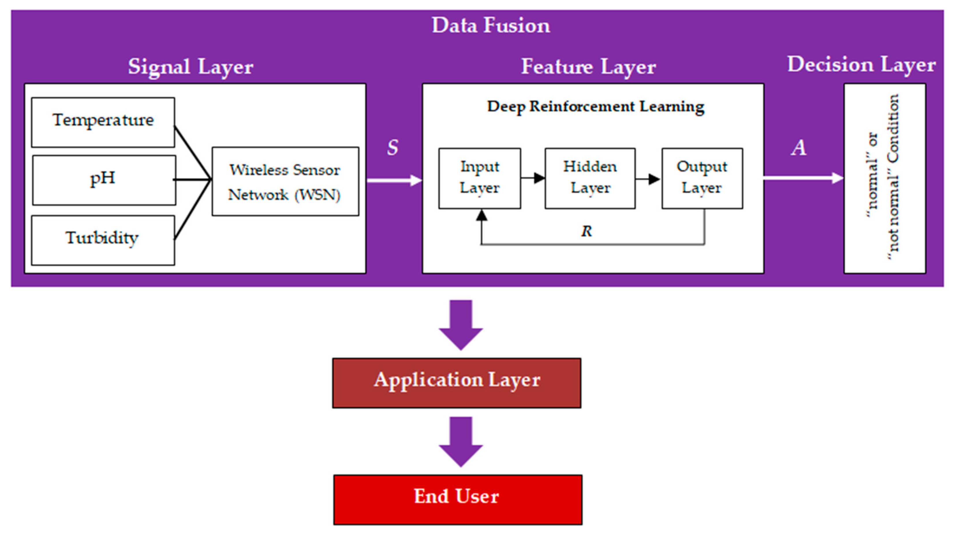
2.6. Combined Data Fusion and Deep Reinforcement Learning Framework

The goal of this study is to combine DF with DRL, in which there is DL to assist agents in determining the actions to be taken. Inside the DF, there is a signal layer that provides state conditions (S) to the feature layer as a DRL trigger to determine what action (A) is performed by the agent. Data processing is done by DL through a neural network consisting of an input layer, a hidden layer, and an output layer. The output layer instructs a reward (R) for the next iteration process, and A is forwarded to the decision layer which translates A as a “normal” or “not normal” condition of data processing. The next layer is the application layer where data are represented in a user interface that can be used by end users. Figure 11 shows a combined DF and DRL visualization:

3. Experimental Method

In this study, the experimental method is an essential part because it forms the foundation for the experimental and analytical processes to produce credible and valuable output. There are several specific goals in the experimental method, which include: (1) validating the sensors’ accuracy, which ensures that the sensors have good quality accuracy, taking into account temperature, real-time data retrieval from fish ponds, and time-series data retrieval; (2) the construction of the deep learning model that is implemented to ensure the validity of the parameters in the class label, the dataset transformation process, and the accuracy of the model used; (3) data fusion algorithm construction, which aims to integrate all layers in the aquaculture monitoring system; (4) application layer environment, which aims to ensure integration to the final process, where an Android-mobile-based user interface is built that can be accessed by end users in real time.

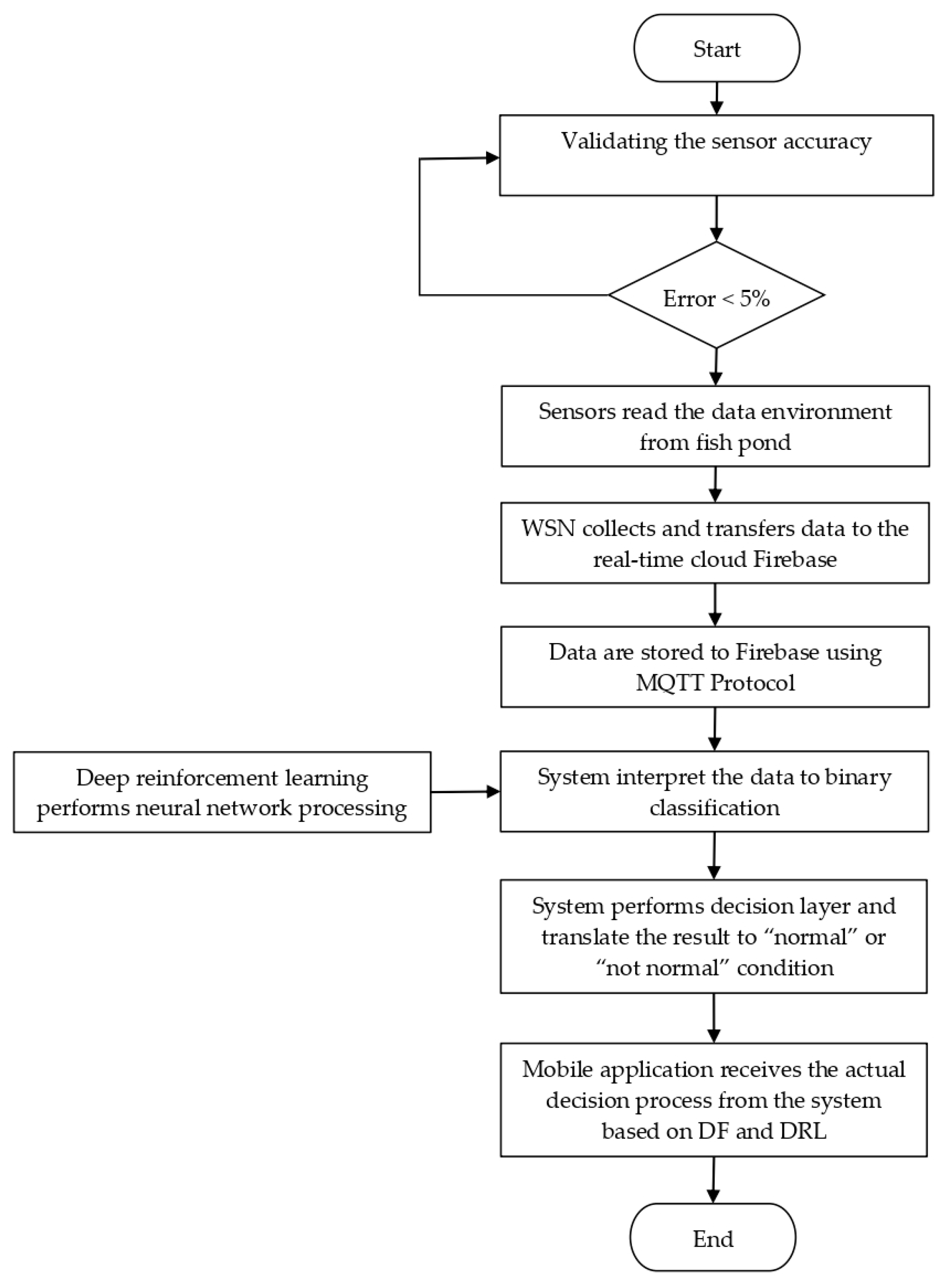
In the experimental process as shown in Figure 12, there are several steps that are carried out. The initial process is carried out by validating sensor accuracy to ensure that the temperature, pH, and turbidity sensor components work properly in order to produce accurate and valid data. The validation process is carried out by testing the sensor in several conditions in the fish pond. The process of collecting test data is carried out with a range of time from morning to evening with eight timeframes beginning from 06.00 am to 08.00 pm. The results of the test are then compared with the measurement results from the measuring instrument, then a gap is sought between the sensor measurement results and the measuring instrument which shows the measurement error range. In this study, the error tolerance given in testing is a maximum of 5% or a minimum of 95% accuracy. If the conditions are not met, then the process will be repeated until it reaches a maximum error of 5%. The system built is a WSN, where the data after being read by the sensor is then transferred to the Firebase real-time cloud which will later be used as the basic parameters for the system to process data. The process of data communication between sensor devices and Firebase is carried out via the message queuing telemetry transport (MQTT) protocol so that data can be transmitted to Firebase to become real-time data. The transferred data in the form of temperature, pH, and turbidity parameters are processed by the deep reinforcement learning (DRL) system through deep learning to produce an action as the output of the agent. In the next stage, the system interprets the data into a binary classification to output 1 or 0. In this stage, DRL implementation is carried out, where the agent provides output based on deep learning modeling that has been embedded in the system. Then, the system performs the decision layer by translating the binary classification into “normal” or “not normal” conditions, where in this study output 0 is defined as a “normal” condition and output 1 is defined as a “not normal” condition. In the final stage, the mobile application receives the actual decision process from the system based on DF-DRL and the real-time conditions of the pond based on parameters of temperature, pH, and turbidity.

Further explanation in Figure 12 relating to the validation of the sensor accuracy, WSNs, modeling of deep learning, and deep learning reinforcement algorithms are explained in detail as follows:

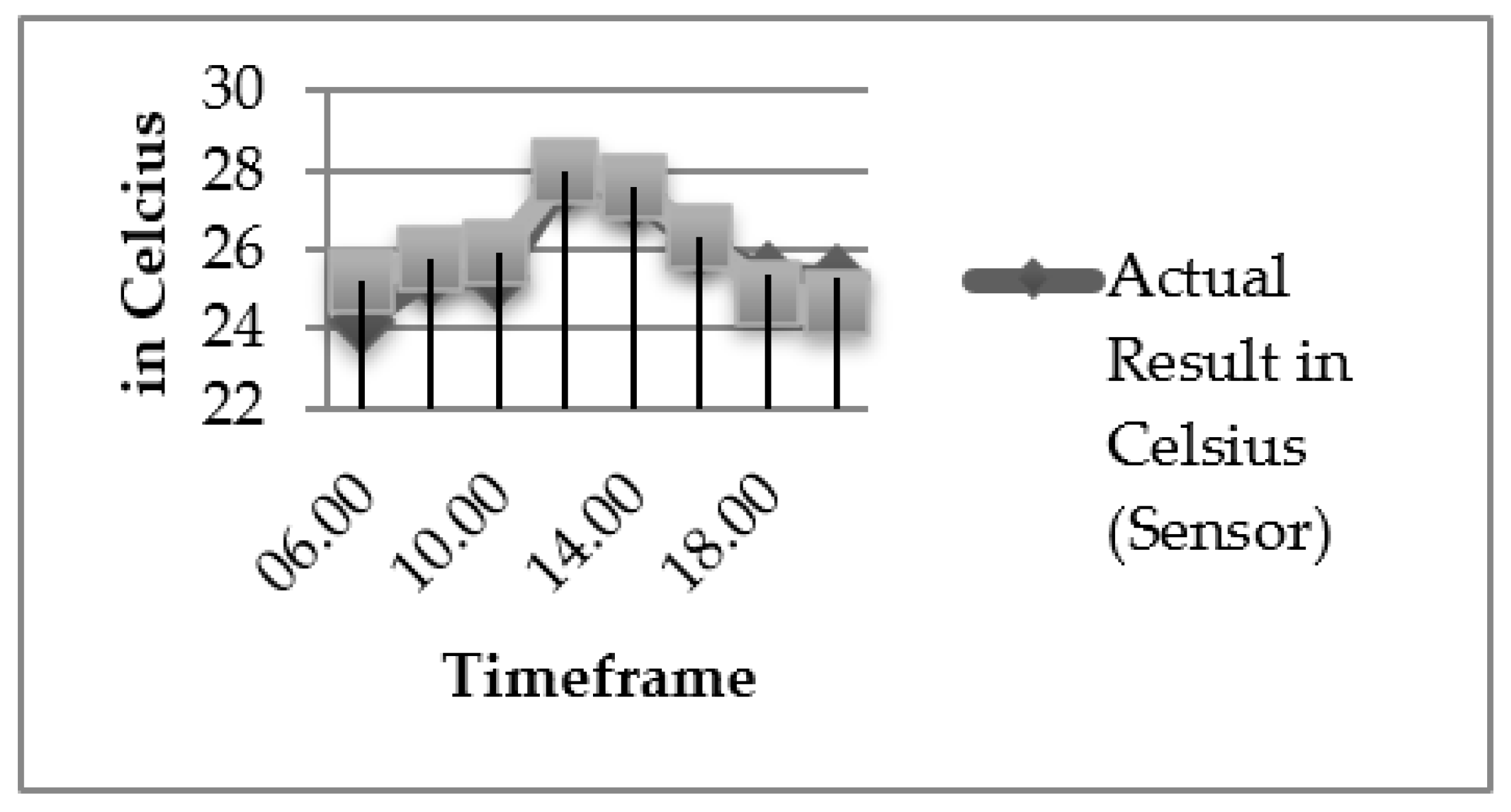
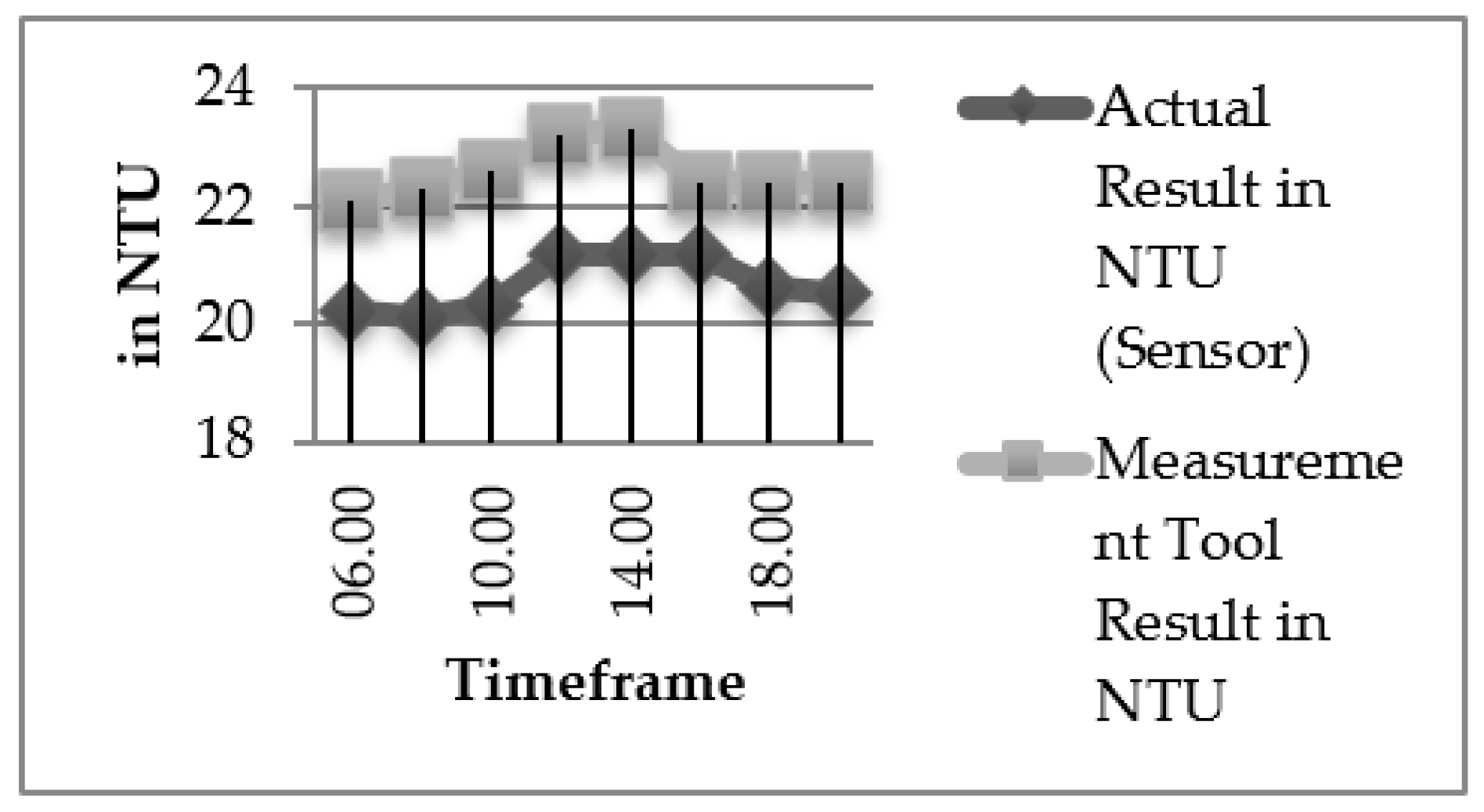
3.1. Validating the Sensor Accuracy

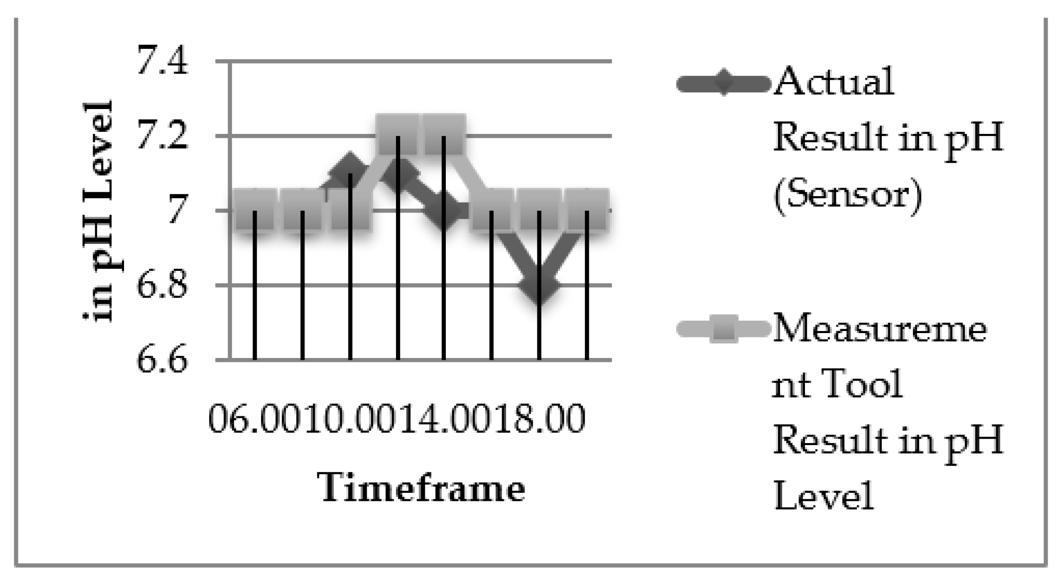
In validating the accuracy of the sensor, it is done by collecting data on the condition of the fish pond which is divided into eight sampling times in the morning, afternoon, and evening with a range of every two hours starting at 06.00 to 20.00 (08.00 pm). At the time of data collection, the environmental conditions were cloudy with occasional light rain, and the air temperature ranged from 25 °C to 30 °C.

Table 1. Timeframe in data collection.

No	Description	Time
1	Part one (morning)	06.00
2	Part two (morning)	08.00
3	Part three (morning)	10.00
4	Part four (noon)	12.00
5	Part five (afternoon)	14.00
6	Part six (afternoon)	16.00
7	Part seven (evening)	18.00
8	Part eight (evening)	20.00

shows a detailed description of the test data collection, which is divided into eight timeframes:

The device configuration in Figure 13 shows the direct interaction of the temperature, pH, and turbidity sensors on the device. The sensor is connected directly to the microcontroller, which is connected to the Wi-Fi module so that the reading data can be accessed in real time.

Testing is carried out by collecting data from the sensor, which is compared with a measurement tool, resulting in a certain error value. At this validation stage, the calculation method is performed using the mean absolute percentage error (MAPE), with the value generated from the sensor being called the prediction value (Pi), while the value generated by the measurement tools is called the actual value (Ai). The difference between Ai and Pi produces an absolute error, which is divided by Ai, so that the MAPE value is formulated in Equation (4), as follows:

MAPE = (1/n) × (Ai − Pi)/Ai

(4)

3.2. The Implementation of WSNs

As described in the previous section, the WSNs in this study integrate sensors to be able to communicate with Firebase cloud data. The process of transmitting sensor data through WSNs is carried out with the pseudocode as shown in

Table 2. Pseudocode data transmission to cloud using WSNs.

BEGIN

initialization WSNs connection

data = read sensor environment [“pH”, “temperature”, “turbidity”]

WSNs send (data) to the cloud

confirmation = cloud receives

IF confirmation = “success” THEN

print “data has successfully sent to cloud” ELSE print “data transmission error” END IF END

to indicate cite Table 2:

The implementation of WSNs for transmitting data from sensors to the cloud can be seen in

Table 3. Real-time data Firebase using WSNs.

ID	Temperature (°C)	Turbidity (NTU)	pH
1	27	28	8
2	20	26	8
3	27	21	8
4	22	26	8
5	26	25	8

, where there is real-time data on the results of environment readings on the pH, temperature, and turbidity parameters.

3.3. Construction of Deep Learning

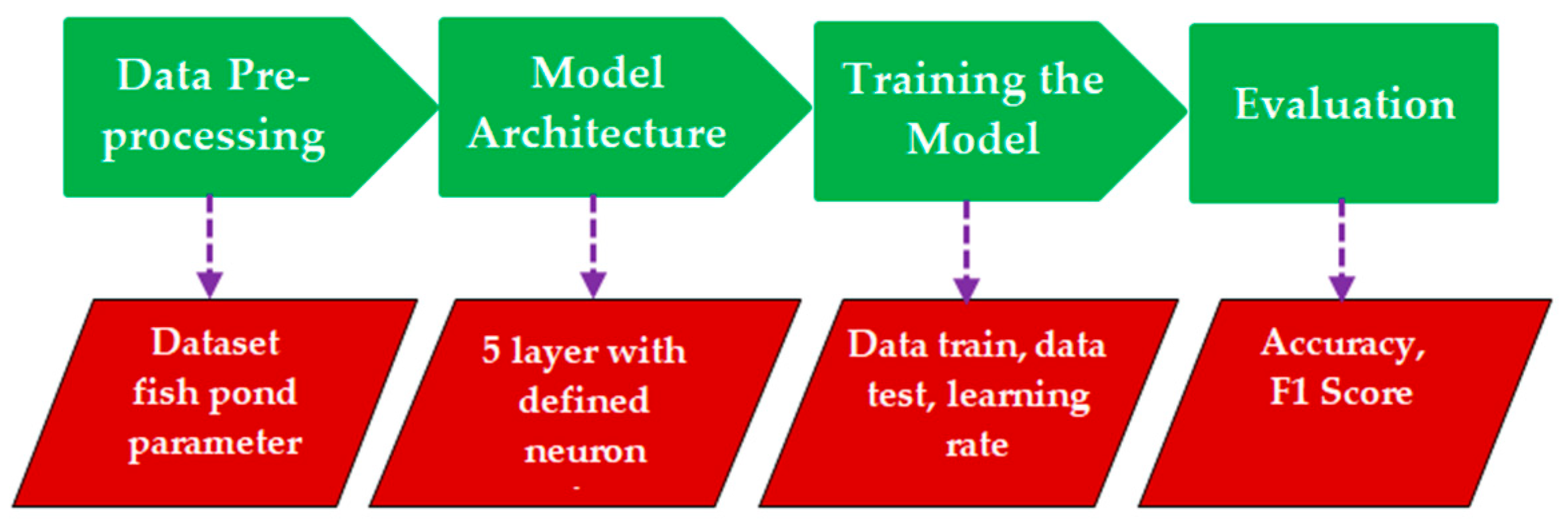
In the development of deep learning, generic stages are used to implement where data pre-processing, model architecture, training the model, and evaluation are carried out. Figure 14 shows a description of each stage in deep learning in this study.

Data pre-processing is carried out by preparing a dataset that will be used in deep learning modeling that uses tabular data derived from various fish pond water conditions, with variations in temperature, pH, turbidity, and “normal” and “not normal” conditions. There are four features in the dataset, consisting of three parameter features, and one classification feature consisting of “normal” and “not normal” labels. The three feature parameters are states, which will later become knowledge for agents in deep reinforcement learning to understand actual environmental conditions so that the agent can decide which action to take under various conditions and at random. As a parameter reference,

Table 4. Fish Pond “Normal” Parameter.

No	Parameter	Range
1	Temperature	25–30 °C
2	pH	6–9
3	Turbidity	0–50 NTU

shows the range of normal conditions of the fish pond environment:

The classification label refers to the parameter conditions in Table 4. For conditions outside of these parameters, the classification label becomes “not normal.” The number of dataset records used in modeling is 1000, consisting of 500 dataset records with a “normal” classification label and 500 dataset records with a “not normal” classification label.

Table 5. Dataset of water condition.

Id	Temperature (t1)	Turbidity (t2)	pH (ph)	Class	Class after Transformation
1	27	15	8	normal	0
2	26	14	7	normal	0
3	20	19	8	not normal (t1)	1
4	19	26	7	not normal (t1)	1
5	28	22	9	normal	0
6	40	27	12	not normal (t1, ph)	1
7	10	30	10	not normal (t1, ph)	1
8	25	21	9	normal	0
9	25	20	9	normal	0
…	…	…	…	…	…
1000	34	52	11	not normal (t1, t2, ph)	1

shows the sample dataset used in the study regarding the “normal” class referred to in Table 4. For example, in ID 1, where the temperature is 27, the turbidity is 15, and the pH is 8, these conditions correspond to the parameter range in Table 4 as “normal” conditions. In contrast, in ID 3, it was found that the temperature was 20, and since it is not included in the parameter range of Table 4, the condition is included in the “not normal” class. Likewise, for ID 7, the value of the temperature is 10, turbidity is 30, and pH is 10. Referring to Table 4, the temperature does not enter “normal” conditions, which are in the range of 25–30 °C, and the pH also does not enter “normal” conditions, which is in the pH range of 6–9. Thus, ID 7 enters the “not normal” classification. In the “class” column in ID 3 and ID 7, both have class conditions of “not normal”, but come from different parameter conditions, where in ID 3, temperature (t1) does not meet “normal” conditions, while in ID 7, temperature (t1) and pH (ph) do not meet “normal” conditions. To facilitate modeling, a classification label is transformed into binary, where “normal” conditions are represented by 0, while “not normal” conditions are represented by 1. The class after transformation is shown in column 6 in gray in Table 5:

The sample data are sufficient for the deep learning algorithm used in the study because the data have gone through the process of data preparation and transformation so that the algorithm has well-balanced data and has no significant noise, especially in this case, which is a binary classification (the condition of the fish pond water is “normal” or “not normal”) also using three clear input parameters i.e., turbidity, pH, and temperature. As described in the previous section, the architecture model uses a deep neural network consisting of five layers. The hidden layer consists of layers, with each neuron having 32 neurons, 16 neurons, and 16 neurons. Furthermore, for the modeling process, dataset training is carried out by dividing the dataset into train data of 80% of the total dataset and test data of 20%. The learning rate used in modeling is 0.01 because this value is generally widely used in various frameworks such as PyTorch and TensorFlow; it also has a balanced value in the sense that it is neither too small nor too big. Specifically, the parameters used in the training model are listed in

Table 6. Training model parameter.

Parameter	Value
train data	80%
test data	20%
learning rate	0.01
epoch	100

below:

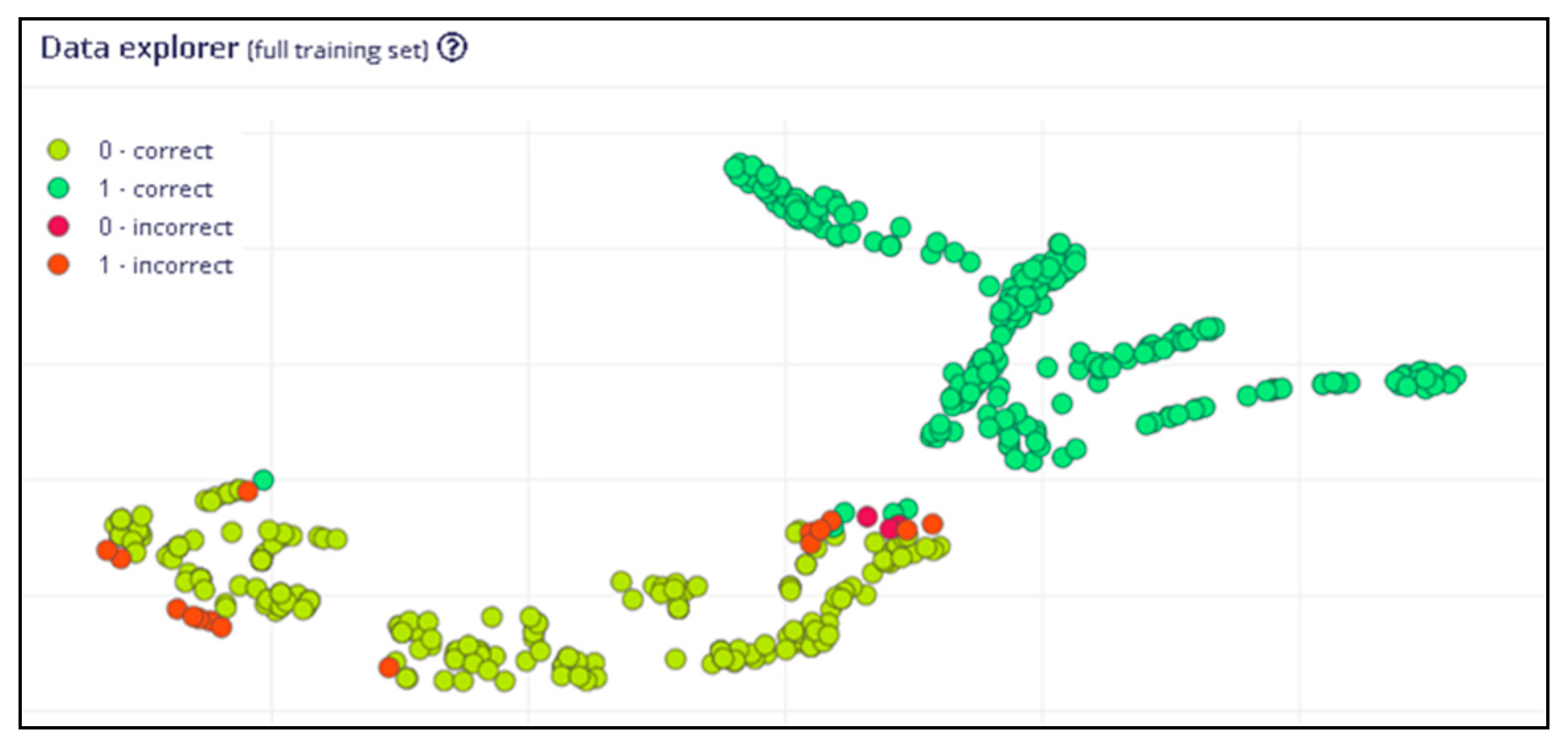
Visually, data exploration from modeling can be seen in Figure 15, where data values 0 and 1 are shown in yellow and green, respectively. It can be seen from the figure that the data are divided into two groups, but there are anomalous data that are indicated by red and orange colors.

From the results of the model training, an evaluation of the model is carried out using accuracy and the F1 score. There are several outputs generated by modeling: true positive (TP), true negative (TN), false positive (FP), and false negative (FN).

Table 7. Confusion matrix.

Condition Status	Count
True Positive (TP)	952
False Positive (FP)	26
True Negative (TN)	974
False Negative (FN)	48

shows the confusion matrix showing TP, TN, FP, and FN:

From the results of the confusion matrix in Table 7 can be calculated accuracy, precision, and recall. While the results of the F1 score are based on calculations from precision and recall, the formulation is shown in Equations (5)–(8):

Accuracy = (TP + TN) + (TP + FP + TN + FN)

(5)

Precision = TP/(TP + FP)

(6)

Recall = TP/(TP + FN)

(7)

F1 Score = 2((Precision.Recall)/(Precision + Recall))

(8)

Therefore, based on the results of the confusion matrix, an accuracy percentage of 96.3% is obtained with a precision of 0.97, a recall of 0.95, and an F1 score of 0.96. The results of deep learning modeling show a percentage greater than 95%; this indicates that the model built has good accuracy for implementation in an aquaculture monitoring system based on DF and DRL.

3.4. Data Fusion Algorithm

Data fusion in this study is a framework that operates the system from integration and signal processing through WSNs contained in the signal layer, processing data obtained from the environment with deep reinforcement learning in the feature layer, as well as interpreting actions that produce output at the decision layer. Algorithmically, the series of processes can be represented by pseudocode as shown in

Table 8. Data fusion pseudo code

BEGIN

Initialize variable: sensor_data; processed_data; model; app

sensor_data --> [turbidity, temperature, pH]

model --> deep reinforcement learning

application --> mobile application

WHILE true

WSNs send (sensor_data) to the cloud <-- signal layer

confirmation = cloud receives

IF confirmation = “success” THEN

print “data has successfully sent to cloud”

ELSE

print “data transmission error”

END IF

preprocessed_data = preprocess(sensor_data) <-- feature layer

train and predict using DRL model

prediction = model.predict(preprocessed_data)

interpret the action based on agent prediction <-- decision layer

fused_data = fuse(prediction)

display result on mobile app <-- application layer

application.display(fused_data)

END

.

3.5. Application Layer Environment

The application layer in this study aims to facilitate communication between the user and the system through the user interface. The application layer is built on a mobile platform so that users can interact with the system anytime and anywhere. The developed system has minimum requirements for installation with the following parameters in

Table 9. Application layer minimum requirement.

Parameter	Specification
Operating System	Android
Version	Ice Cream Sandwich (4.0)
Random Access Memory	1 GB
Storage Space	Free Space minimum 100 MB
Processor	1 GHz

:

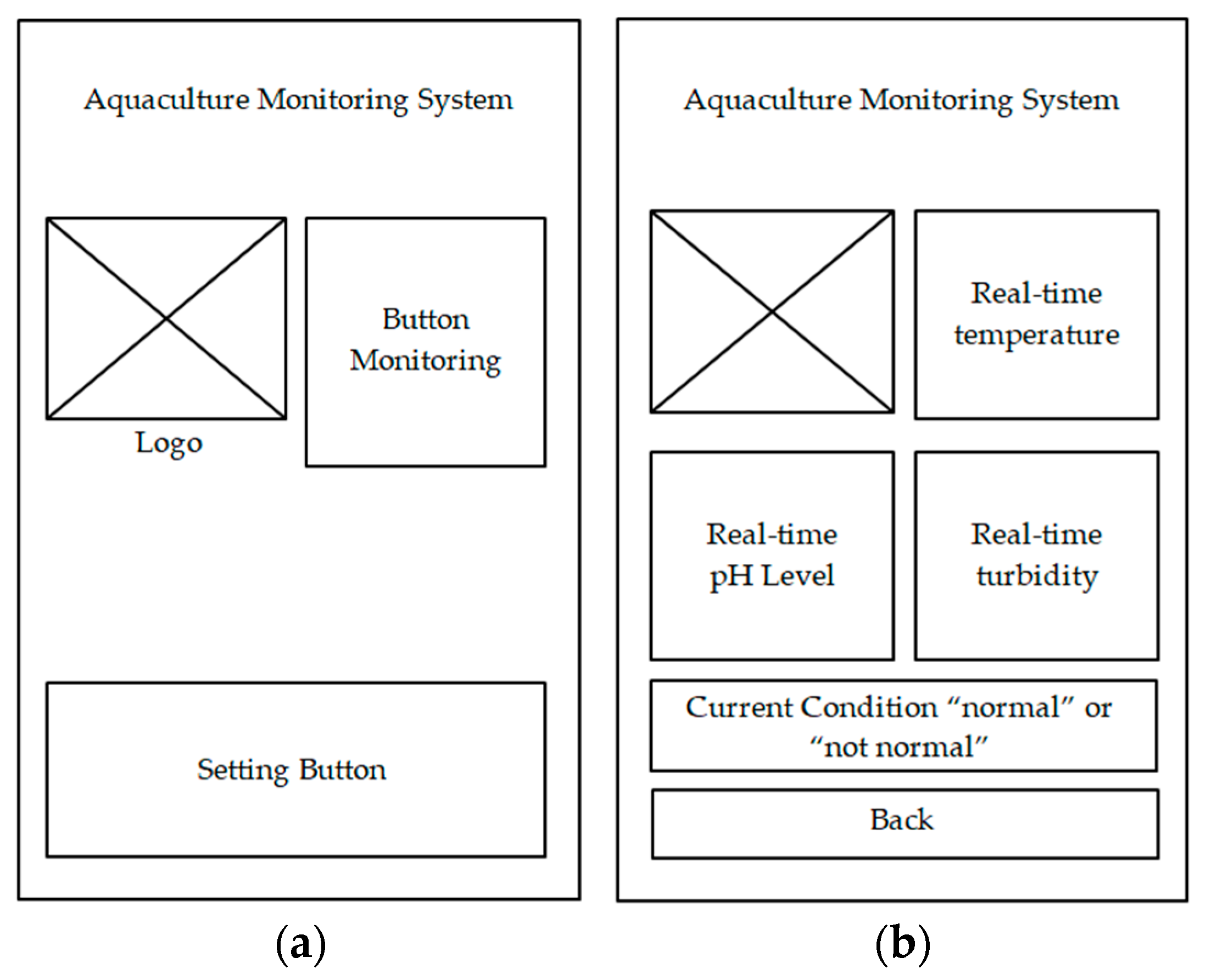
The user interface was developed with the Android Studio Integrated Development Environment (IDE) which was designed to consist of a main menu which can be seen in Figure 16a and a monitoring menu in Figure 16b.

Meanwhile, the implementation of the user interface display of the aquaculture monitoring system can be seen in Figure 17a,b, where there is a display of the main menu and monitoring menu.

4. Results and Discussions

This section discusses experimentation and analysis from several points of view, each with specific goals: (1) an analysis of the accuracy of sensors is carried out to find out how accurate the sensors implemented in the system are; (2) by carrying out a comparative analysis between the implemented deep learning model and the traditional learning model, it aims to see the effectiveness and accuracy of the model implemented in the system when compared to other models; (3) by comparing a system based on data fusion-deep reinforcement learning (DF-DRL) with a system based on a rule-based algorithm, the aim is to find out how the level of accuracy of the proposed system compares to conventional systems in the form of a rule-based algorithm system; (4) see how cost-effective the DF-DRL system is when compared to a labor-based system. Figure 18 shows the specific goal of the analysis:

4.1. Analysis of the Accuracy of Sensors

The sensor measurement results consist of measurements of temperature, pH level, and turbidity, which are carried out directly on the fish pond water. In temperature measurements for eight timeframes, there are actual results that come from sensors and measurement results obtained from measurement tools as shown in

Table 10. The result of temperature measurement.

Timeframe	Actual Result in Celsius (Sensor)	Measurement Tool Result in Celsius	Absolute Gap Value	Error Percentage
06.00	24.2	25.2	1.0	3.97%
08.00	25.4	25.8	0.4	1.55%
10.00	25.3	25.9	0.6	2.32%
12.00	27.8	28.0	0.2	0.71%
14.00	27.4	27.6	0.2	0.72%
16.00	26.1	26.3	0.2	0.76%
18.00	25.4	24.9	0.5	2.01%
20.00	25.3	24.7	0.6	2.43%
		Average Error		1.81%

. The absolute gap value generated by measurements using sensors and measurement tools has the highest value of 1.0 at the 06.00 timeframe, where the sensor measurement results show 24.2 °C and the measurement tool results show 25.2 °C. The gap value between the two measurements is 1 °C and then it is used as a value to determine the percentage error, by dividing the absolute gap value by the measurement tool result value, with value 1.0 divided by 25.2, resulting in a percentage error of 3.97%. The lowest percentage error is produced on the 12.00 timeframe of 0.71%. Overall, the average error percentage on the results of temperature measurements is 1.81%, which means that this percentage is the value of MAPE.

Visually, the results of sensor measurements and measurement tools can be seen in Figure 19, where in both measurements, there is an increase in temperature ahead of the 10.00 timeframe, then it rises significantly at 12.00 with temperatures around 28 °C. Then, it drops slowly from the 14.00 to 20.00 timeframe.

The turbidity measurement results are shown in

Table 11. The result of turbidity measurement.

Timeframe	Actual Result in NTU (Sensor)	Measurement Tool Result in NTU	Absolute Gap Value	Error Percentage
06.00	20.2	22.1	1.9	8.60%
08.00	20.1	22.3	2.2	9.87%
10.00	20.3	22.6	2.3	10.18%
12.00	21.2	23.2	2.0	8.62%
14.00	21.2	23.3	2.1	9.01%
16.00	21.2	22.4	1.2	5.36%
18.00	20.6	22.4	1.8	8.04%
20.00	20.5	22.4	1.9	8.48%
		Average Error		8.52%

with the nephelometric turbidity unit (NTU) measurement unit. The highest absolute gap value is found in the 10.00 timeframe of 2.3 NTU, which means an error percentage of 10.18%. Meanwhile, the lowest absolute gap value on the timeframe is 1.2 NTU, or an error percentage of 5.36%. The MAPE generated from turbidity measurements is 8.52%.

Figure 20 shows the visualization of turbidity measurement from the timeframe 06.00 to 20.00. In the timeframe 12.00 to 14.00 there is an increase in the level of turbidity because at that time it is the time for fish feeding, so the turbidity level increases.

Table 12. The result of pH level measurement.

Timeframe	Actual Result in pH Level (Sensor)	Measurement Tool Result in pH Level	Absolute Gap Value	Error Percentage
06.00	7.0	7.0	0.0	0.00%
08.00	7.0	7.0	0.0	0.00%
10.00	7.1	7.0	0.1	1.43%
12.00	7.1	7.2	0.1	1.39%
14.00	7.0	7.2	0.2	2.78%
16.00	7.0	7.0	0.0	0.00%
18.00	6.8	7.0	0.2	2.86%
20.00	7.0	7.0	0.0	0.00%
		Average Error		1.06%

shows the result of the pH level measurement, with the highest absolute gap value of 0.2 in the timeframe of 14.00 and 18.00, while the highest percentage error was 2.86% at 18.00. This percentage error is generated from the absolute gap value, which is 0.2, divided by the measurement tool result, which is 7.0. Meanwhile, when compared with testing on the timeframe of 14.00, the absolute gap value is 0.2 divided by the measurement tool result of 7.2, which produces an error percentage of 2.78%. The resulting error percentage for the timeframe of 14.00 is lower than that of the timeframe of 18.00. Therefore, the highest percentage error at the pH level measurement is at the timeframe of 18.00, at 2.86%, where the actual result on the sensor resulted in a pH level reading of 6.8, but the measurement tool showed a pH level of 7.0. Overall, MAPE is produced at a pH level of 1.06%.

In Figure 21, the visualization of the pH level measurement between the sensor and measurement tools shows that there is not really a significant gap.

The percentage accuracy results from the three sensor readings are then averaged to determine the overall accuracy of the aquaculture monitoring system device. Overall, of the three components measured based on the percentage error, it resulted in the average of 3.80%.

Table 13. Average error of all components.

Description	Error Percentage
Temperature	1.81%
pH Level	1.06%
Turbidity	8.52%
Average Error of All Components	3.80%

shows the total percentage error of the components observed.

4.2. Comparison of Deep Learning and Traditional Learning Model

The implementation of deep learning in this research requires further studies related to the effectiveness and accuracy of the resulting model. Therefore, a comparative analysis was carried out between deep learning modeling and traditional learning models with supervised learning or classification types. Several previous studies used traditional machine learning in modeling, including support vector machine [41], k-nearest neighbor [42], and naïve Bayes classifier [43]. The three models are implemented in the case of a model built with a modeling process in several stages, including (1) preparing the same dataset used in deep learning modeling, the fish pond parameter dataset, consisting of four features divided into three feature parameters (temperature, pH, and turbidity), class features consisting of “normal” and “not normal” labels, and data of 1000 records consisting of 500 “normal” labels and 500 “not normal” labels; (2) data transformation process by converting “normal” labels with 0 and “not normal” with 1; (3) model implementation with 80% train data and 20% test data; (4) evaluation process through the accuracy parameters of each model. After the modeling stages are carried out, the accuracy value of the model is generated, as shown in

Table 14. Model accuracy performance.

Model	Accuracy Percentage
Study I (Support Vector Machine) [41]	95.75%
Study II (k-Nearest Neighbor) [42]	92.15%
Study III (Naïve Bayes Classifier) [43]	95.02%
Average Accuracy	94.31%

below:

Of the three models compared, the highest accuracy value is study I using the SVM model which has an accuracy percentage of 95.75%, while the lowest is study II which uses KNN with an accuracy percentage of 92.15%. The average accuracy of the three models is 94.31%. When compared to the deep learning model implemented in modeling, it has a higher accuracy rate of 96.30% or so based on a comparative analysis between deep learning and traditional learning models; in the context of this research, the deep learning modeling has better accuracy than traditional learning models. Visually, the model comparison can be seen in Figure 22 below:

4.3. Comparison DF-DRL and Rule-Based Algorithm

To validate the implementation of DF-DRL in the aquaculture monitoring system, a comparative analysis was carried out using a rule-based algorithm method. The first step is to determine the normal conditions as shown in Table 4 as an indicator of the “true” condition; apart from these conditions, it is stated in “false”. The second step is the rule-based algorithm coding process that is embedded in the system. The third step is the development of test scenarios with various conditions of temperature, pH, and turbidity for 20 test conditions. The testing process is carried out under different conditions on several water samples; for example, scenario 1 and scenario 2 are scenarios taken from the same testing water sample, as are several other scenarios that are the results of testing from different water samples. The purpose of the testing is to see how the system is able to adapt to a random environment. Tests were carried out using an aquaculture monitoring system based on DF-DRL and a rule-based algorithm. The test scenarios along with the test results are represented by

Table 15. Scenario and result testing.

Scenario ID	Condition			Expected Value	DF-DRL	Rule-Based Algorithm
	Temperature	Turbidity	pH
1	26	21	8	normal	normal	normal
2	26	20	8	normal	normal	normal
3	25	21	7	normal	normal	normal
4	27	19	9	normal	normal	normal
5	27	21	8	normal	normal	normal
6	30	35	9	normal	normal	normal
7	30	42	8	normal	not-normal	normal
8	30	47	8	normal	normal	normal
9	28	45	9	normal	normal	normal
10	24	45	8	normal	normal	normal
11	21	25	7	normal	normal	normal
12	21	30	7	normal	normal	normal
13	27	26	8	normal	normal	normal
14	20	29	8	normal	normal	normal
15	20	26	7	normal	normal	normal
16	40	22	7	not normal	not normal	normal
17	24	40	10	not normal	not normal	normal
18	33	8	8	not normal	not normal	normal
19	10	53	9	not normal	not normal	not normal
20	17	30	5	not normal	not normal	not normal

below:

In Table 15, the actual value is shown by the “expected value” column, which is the reference for the condition of the fish pond. In the DF-DRL column, out of the 20 scenario conditions tested, there is one condition (which is indicated with red font) that does not match the expected value, so that the total value that corresponds is 19 conditions. Furthermore, the cause of this anomaly condition occurs because it is predicted due to two factors: first, the temperature and turbidity level are almost close to the threshold, so the model is confused about whether the condition is “normal” or “not normal”, and second, the MAPE tolerance on the sensor is 3.8% so that the sensor reading when testing the DF-DRL is close to the condition “not normal” and the system detects the condition as “not normal”. Then, from the 19 true conditions, divide by the number of 20 scenarios to produce 95% accuracy. Meanwhile, in the rule-based algorithm column, there are 17 conditions that have appropriate values and 3 conditions that do not match; this case can also be caused by the condition values that are close to the threshold. Therefore, the rule-based algorithm produces a percentage accuracy of 85%; a brief comparison of the two methods is shown in

Table 16. Comparative result of DF-DRL vs. rule-based algorithm.

Method	Total Expected Value	Correct Value	Incorrect Value	Accuracy Percentage
DF-DRL	20	19	1	95%
Rule-Based Algorithm	20	17	3	85%

:

4.4. Analysis of DF-DRL Implemented in Aquaculture Monitoring System

The implementation of DF-DRL in the aquaculture monitoring system has a significant impact on fish cultivators and provides efficiency and ease in managing low-cost aquaculture. The analysis was carried out by comparing the aquaculture monitoring system based on DF-DRL technology with the labor force. Calculations are made by looking at conditions in Indonesia, where electricity costs are charged at IDR 1352 per kWh, or IDR 1.352 per Wh. The maximum power usage for the DF-DRL device is 20 watts with daily use for 24 h. Meanwhile, the daily labor force fee is IDR 50,000 with duration of 3 to 5 h.

Table 17. Analysis DF-DRL compared with labor force.

Method	Component	Daily Cost (IDR)	Monthly Cost (30 Days—IDR)	Maintenance (IDR)	Total (IDR)	In USD (1 USD = 15,000)
DF-DRL	20 Watt|IDR 1.352 per Wh	648.960	19,468.8	50,000	69,468.8	4.63
Labor Cost	Labor Cost = IDR 50,000	50,000	1,500,000	-	1,500,000	100

shows a comparative analysis of the cost burden between DF-DRL technology and the labor force in the aquaculture monitoring system.

In Table 17, it can be seen that there is a significant comparison between DF-DRL technology and labor costs in the aquaculture monitoring system. In the daily cost column, the use of DF-DRL for 24 h is IDR 648.960; if accumulated within 1 month (30 days) it will result in a cost of IDR 19,468.8. Meanwhile, the labor cost for a month is IDR 1,500,000. Maintenance costs are an additional parameter for DF-DRL technology of IDR 50,000. Consequently, the total cost incurred each month for DF-DRL technology is IDR 69,468.8 or USD 4.63 per month. Meanwhile, the total labor cost is IDR 1,500,000 or USD 100 per month. From this analysis, it can be concluded that the implementation of DF-DRL technology in aquaculture monitoring systems provides low-cost benefits and added value for fish cultivators.

5. Conclusions

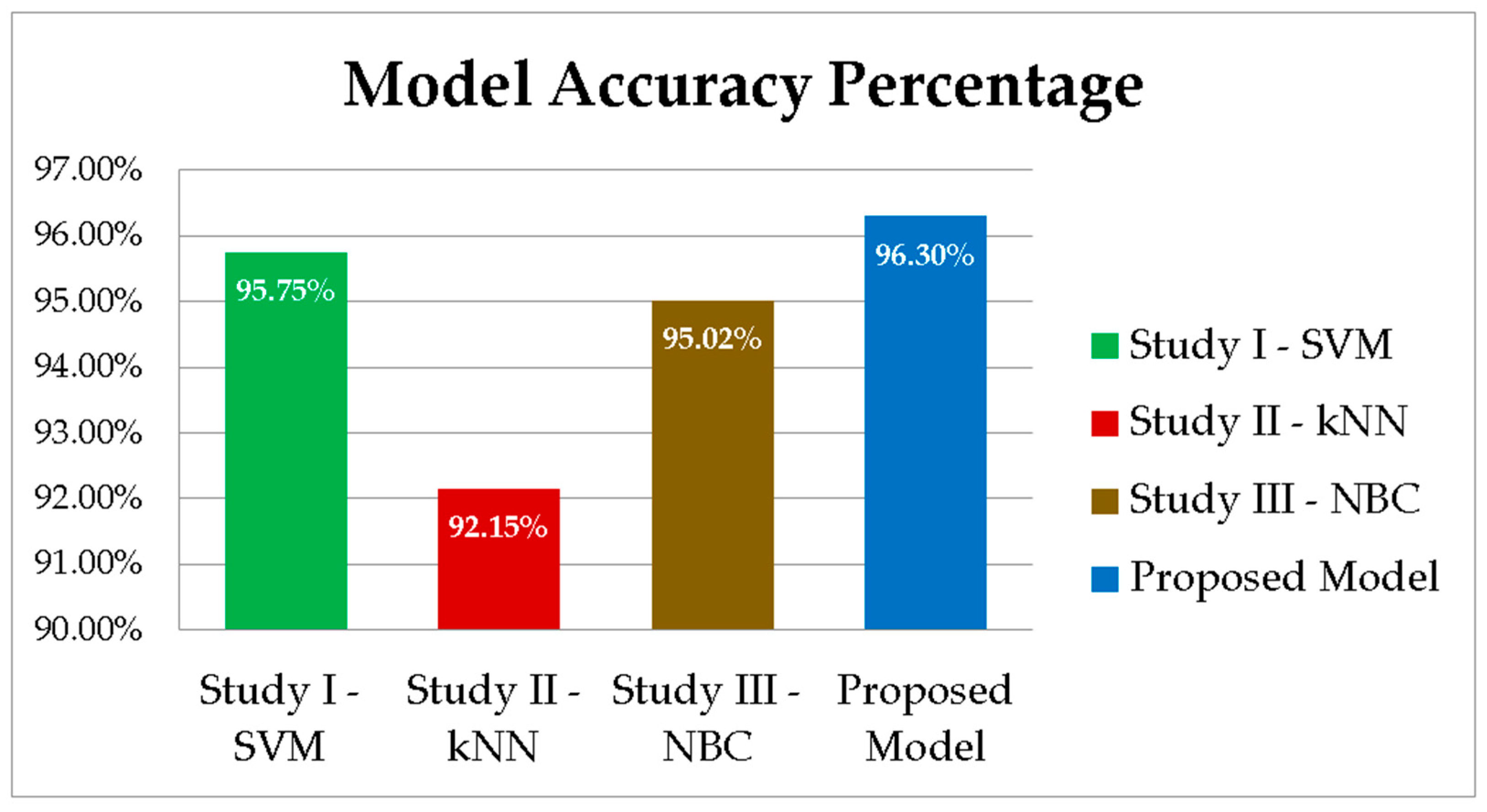
DF-DRL technology in the aquaculture monitoring system provides efficiency in the accuracy of the data generated by the system and the reliability of data that can be accessed in real time. The stage is carried out by testing the quality of sensor accuracy on WSNs, where it is obtained with an average error in MAPE of 3.80% or an accuracy of 96.2%. From the aspect of deep learning modeling, a comparative analysis has been carried out with traditional machine learning consisting of a support vector machine (SVM), k-nearest neighbor (kNN), and naïve Bayes classifier (NBC), with an average accuracy of 94.31%, while the results of deep learning modeling accuracy implemented in this study are 96.30%. Meanwhile, the effectiveness of DF-DRL performance with a rule-based algorithm with testing of 20 scenarios resulted in 95% and 85% accuracy, respectively. DF-DRL technology has 10% higher performance than rule-based algorithms.

While the DF-DRL analysis in terms of cost effectiveness is compared to labor cost through the monthly cost parameter, it is found that DF-DRL technology is far superior to labor cost, which is USD 4.63 for DF-DRL technology and USD 100 for labor cost in monthly cost. DF-DRL technology is an alternative in a low-cost aquaculture monitoring system with technology that produces significant data accuracy and validity. In future development, the system can be integrated with various sensors, such as hungry fish detectors, monitoring cameras integrated with image processing, actuators that provide automatic feeding, and various other sensors and actuators that are adaptive to various environmental conditions.