A Cascade Network for Blind Recognition of LDPC Codes

Abstract

Coding blind recognition plays a vital role in non-cooperative communication. Most of the algorithm for coding blind recognition of Low Density Parity Check (LDPC) codes is difficult to apply and the problem of high time complexity and high space complexity cannot be solved. Inspired by deep learning, we propose an architecture for coding blind recognition of LDPC codes. This architecture concatenates a Transformer-based network with a convolution neural network (CNN). The CNN is used to suppress the noise in real time, followed by a Transformer-based neural network aimed to identify the rate and length of the LDPC codes. In order to train denoise networks and recognition networks with high performance, we build our own datasets and define loss functions for the denoise networks. Simulation results show that this architecture is able to achieve better performance than the traditional method at a lower signal-noise ratio (SNR). Compared with the existing methods, this approach is more flexible and can therefore be quickly deployed.

1. Introduction

Forward error correcting codes counteract the random errors over the noisy channel by inserting redundant bits into code words [1]. In order to balance the quality and rate of communication, different coding schemes have been proposed over the past few decades, and the corresponding decoding scheme has increasingly attracted the attention of many researchers. In the traditional communication system, only the decoder knows the encoding parameters it can decode accurately. However, under the conditions of non-cooperative communication [2], such as cognitive radio, it is impossible for the non-cooperative receiver to decode without prior knowledge of the code parameters. Hence, coding blind recognition is urgently required, and has attracted extensive research interest [3].

Among the existing coding schemes, Low Density Parity Check (LDPC) code, which was first proposed by Gallager in the 1960s [4], has been widely used in modern communication systems, and has been identified as the long code coding scheme in the 5G enhanced mobile broadband scene due to its long code length, rich combination, and sparse check matrix. Since LDPC codes have these basic characteristics, it also poses a challenge to decoding and coding blind recognition. In practical terms, LDPC codes are usually too long to reconstruct the parity-check matrix directly.

In order to solve the problem of high time complexity and high computational complexity, most of the existing methods of LDPC coding blind recognition proposed in recent years use closed set identification. The identification methods based on the closed set utilize a known set which contains all probable parameters [5,6,7,8]. The log likelihood ratio (LLR) used in [5,6] for coding blind recognition performs well at a low SNR. In [7], LDPC code is identified by the average likelihood difference (LD) of parity-checks. Since the LLR of syndrome a posterior probability is widely used in these methods, it is often limited by channel conditions. Wu proposed to calculate the average cosine conformity (CC) for recognition, which not only has an explicit probability density, but also has low computational complexity [8]. The code parameters within a given closed set can be recognized using the methods above. However, the identification methods without a candidate set are more universal, and take a longer time to calculate. The minimum Hamming weight vector is used in the search algorithm proposed by Valembois [9], but the fault tolerance capability is weak. Cluzeau used iterative coding [10] to improve the tolerance of the method in [9] followed by the problem of longer time consumption for finding sparse parity-check vectors.

Deep learning as an emerging technique has been widely applied in the many fields, such as image classification [11] and natural language processing [12]. The best solutions are found in specific problems through the connection of multi-layer networks. Different network models have been proposed by scholars in different fields—e.g., the Transformer model proposed by A. Vaswani [13] is a well-known sequence to sequence (seq2seq) architecture that performs well by treating a sentence as a sequence of words in the field of natural language processing (NLP). The self-attention layer structure in the Transformer greatly reduces computation time using the trick of parallel calculation.

In recent years, the combination of neural networks and coding blind recognition has progressed rapidly [14,15,16,17]. It has been proven that both of the coding schemes and the coding parameter are able to be identified using neural networks [14]. Two types of LDPC codes can be identified in [15], while a 2-dimensional convolution neural network is used to identify the parity-check matrix of LDPC codes with the help of a candidate set [16]. Moreover, a joint modulation and channel coding recognition framework is proposed in [17] for the practical 5G-PDSCH protocols using the novel Res-Inception convolutional NN and the algorithm based on maximal ALLR. Inspired by the deep learning model used in NLP, we propose a novel method based on Transformer for recognizing the coding parameter of LDPC codes.

Furthermore, channel condition is the key factor in coding blind recognition. Almost all of the traditional coding blind recognition methods of LDPC codes adequately utilize the channel condition. On the contrary, most existing recognition methods based on deep learning pay little attention to the channel condition, which made these deep learning methods identify accurately at high SNR but fare badly when the channel condition is not good enough. Channel noise is similar to image noise in some areas. The deep learning method for two-dimensional image denoising has been widely studied in the field of computer vision [18], and has made considerable progress over the last couple of years [19,20]. In addition to this denoising, the design aims for two-dimensional data. Denoising networks are also widely used in other fields. In the area of decoding, a novel receiver architecture [21] concatenates a belief propagation (BP) decoder for decoding with a convolution neural network (CNN) for denoising. The iteration between BP decoding and CNN will gradually improve the SNR, and achieve better decoding performance. In [22], the double-CNN denoiser is designed to surpass the noise by estimating the channel state information (CSI) under the Rayleigh fading channel. However, these two methods can hardly be applied in practical terms due to the constraint of the information bit length [23], which can cause the dimension explosion of the neural network.

In this paper, we design a deep-learning-based architecture for coding blind recognition of LDPC codes under an additive white Gaussian noise channel with different SNRs. Briefly, the main contributions of this paper include: The code words are treated as a sequence of words which is sent to the proposed Transformer-based neural network for coding blind recognition. A denoising network and new loss functions are proposed in order to get reliable recovery of the bit stream for recognition. Besides, the denoising network and blind recognition network are cascaded, and the simulation results show that the accuracy of the cascade structure is better than that of the non-cascade structure. Furthermore, we compared the proposed method with traditional methods. When the SNR is low, our method performs better than the traditional one.

2. Related Work

In this section, the communication principles of typical digital systems and the location of blind recognition in the communication system are briefly introduced. In order to illustrate our method clearly, the encoding method of the LDPC code and the basic knowledge of the neural network related to this design are introduced.

2.1. Communication System

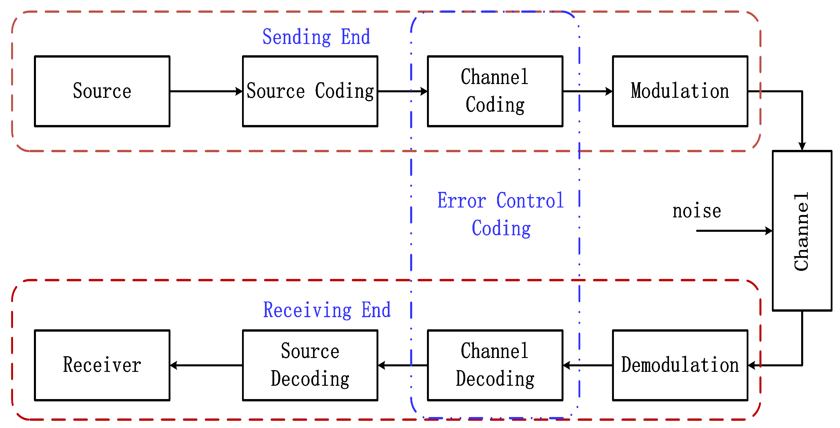
The typical digital system communication block diagram is shown in Figure 1. The binary information sequence after the source coding is converted into code word information by means of channel coding. The code words are then converted into a waveform signal that can be transmitted on the channel after modulation. During the transmission, the signal is interfered with by various noises, so that the waveform information received by the demodulator may be wrong. When the information from the channel is transmitted to the receiving end, it will firstly be demodulated, and then enter the channel decoding module.

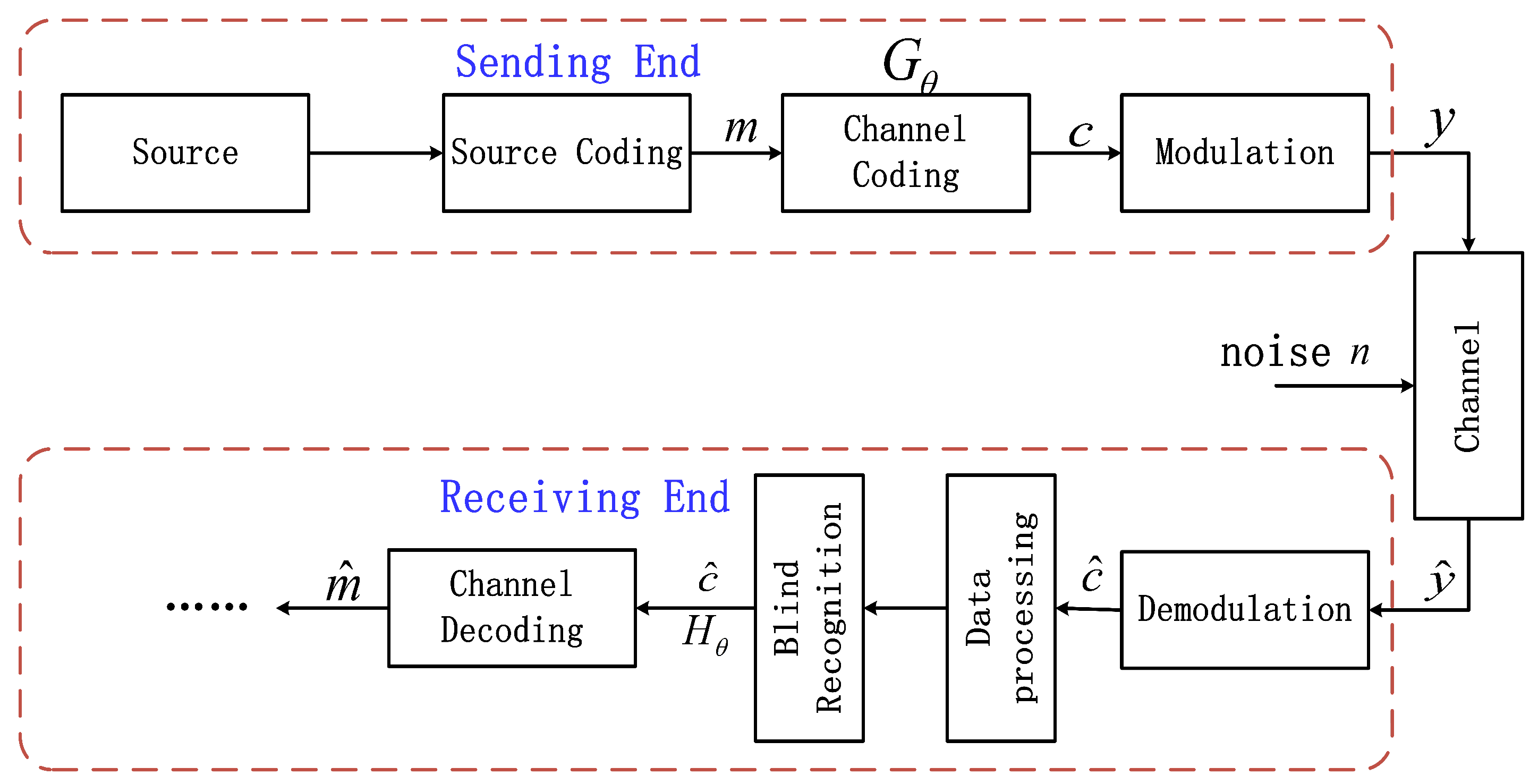
In cooperative communication, the decoding module knows the channel conditions and encoding parameters used for real-time communication. In contrast, coding parameters need to be identified in non-cooperative communication before decoding. The block diagram of a typical non-cooperative communication system is shown in Figure 2.

2.2. Basic Theory of LDPC Code

LDPC code is a linear block code whose parity-check matrix contains only a few non-zero elements. The selection of check matrix is very important for LDPC codes, which can not only affect the error correction ability, but also can affect the complexity of LDPC encoding and decoding. The theoretical analysis and formula derivation in this section are all based on Error Control Coding [24].

As shown in Figure 2, $G^{\Theta }=\left\{G^1,G^2,\cdots ,G^N\right\}$ represents the set of encoders, where N is the number of generator matrix, and G represents the generation matrix of size $\left(k,n\right)$. The encoder is switched by the transmitter according to the channel conditions. At the sending end, original bits are divided into A groups, and each group has a length of k. The ith information $m_i=\left[m_{i,1},m_{i,2},\cdots ,m_{i,k}\right]$ is sent into encoder with n-bits code word $c_i=\left[c_{i,1},c_{i,2},\cdots ,c_{i,n}\right]$ output, where $m_{i,j},c_{i,j}\in GF\left(2\right)$.The encoding formula is shown in (1):

$$c_i=m_i·G$$

(1)

The parity check matrix H of size $\left(n-k,n\right)$ satisfies $c_i·H=0$. Since H is a dual matrix of G, the reconstruction of H and G carries the same meaning for blind recognition of LDPC code. In binary phase-shift keying (BPSK) modulation, the result can be expressed as

$$y=2c_i-1$$

(2)

After modulation, channel transmission, and demodulation, the code word $\widehat{c}$ is sent to the receiving end for decoding. The additive white Gaussian noise (AWGN) of n with zero-mean and variance of ${\sigma }^2$ is considered in this paper. $\widehat{c}$ can then be represented by

$$\widehat{c}=y+n$$

(3)

Traditional soft decision for decoding is to calculate the LLR using the prior information of channel condition.

$${\mathrm{LLR}}_i=ln\left(\frac{P\left(c\left[i\right]=0|\widehat{c}\left[i\right]\right)}{P\left(c\left[i\right]=1|\widehat{c}\left[i\right]\right)}\right)$$

(4)

where $P\left(c\left[i\right]=0|\widehat{c}\left[i\right]\right)$ and $P\left(c\left[i\right]=1|\widehat{c}\left[i\right]\right)$ donate the probability of $c\left[i\right]$ to be considered as 0 and 1 at the receiver with a known channel condition. When channel is AWGN, we get:

$$P\left(c\left[i\right]=0|\widehat{c}\left[i\right]\right)=\frac{e^{-2·\widehat{c}\left[i\right]/{\sigma }^2}}{1+e^{-2·\widehat{c}\left[i\right]/{\sigma }^2}}$$

(5)

Substitute (5) for (4). The LLR is represented as follows:

$${\mathrm{LLR}}_i=-2·\frac{\widehat{c}\left[i\right]}{{\sigma }^2}$$

(6)

LLR is then used for decoding or blind recognition. Furthermore, LLR can be also used for describing the relationship H and $\widehat{c}$.

2.3. Deep Learning Method

In this subsection, we introduce the basic theory of CNN and Transformers, and then give some examples of the applications of CNN in the area of coding blind recognition.

2.3.1. Convolution Neural Networks

The CNN is mainly composed of convolution layers, pooling layers, and fully connected layers. The features of adjacent data are extracted by convolution layer. Pooling layer retains the main feature, and reduces the number of parameters. The cascade of convolution layer and pooling layer transforms local features into global features. Finally, the fully connected layer takes the global feature as the input and the prediction result as the output. The CNN is widely used in computer vision.

In [16], authors use CNN for LDPC code blind recognition with the help of closed set. It firstly receives the output sequence. The output sequence $\widehat{c}$ processed by LLR generators is described by (6). In order to make better use of LLR, this method utilizes LLR of syndrome a posteriori probability (SPP) [7],

$${\varphi }_{i,j}^{\theta }=2arctanh\left(\prod _{\lambda \in \left\{\mathsf{\Lambda }\right\}}tanh\left(L\left(\widehat{c}\left[\lambda \right]\right)/2\right)\right)$$

(7)

and then get the set of SPP vectors $\mathsf{\Phi }=\{{\varphi }^1,{\varphi }^2,\cdots ,{\varphi }^N\}$. The elements $\varphi =\{{\varphi }_1^{\theta },{\varphi }_2^{\theta },\cdots ,{\varphi }_{(n-k)}^{\theta }\}$ in $\mathsf{\Phi }$ are generated by parity-check matrix H and different channel conditions. Since the size of parity-check matrices H is different, $\varphi$ is of different length correspondingly. In order to get feature matrix F, each $\varphi$ picks $\alpha$ elements randomly, where $\alpha$ is the smallest length of $\varphi$. Obviously, F is of size $\alpha \times N$. Finally, F is sent to blind recognition network for recognition. Since it considers channel condition within known data sets, the calculation of SPP with different LLR will cause a waste of time. This method cannot applied in the real scene.

2.3.2. The Model Architecture of the Transformer

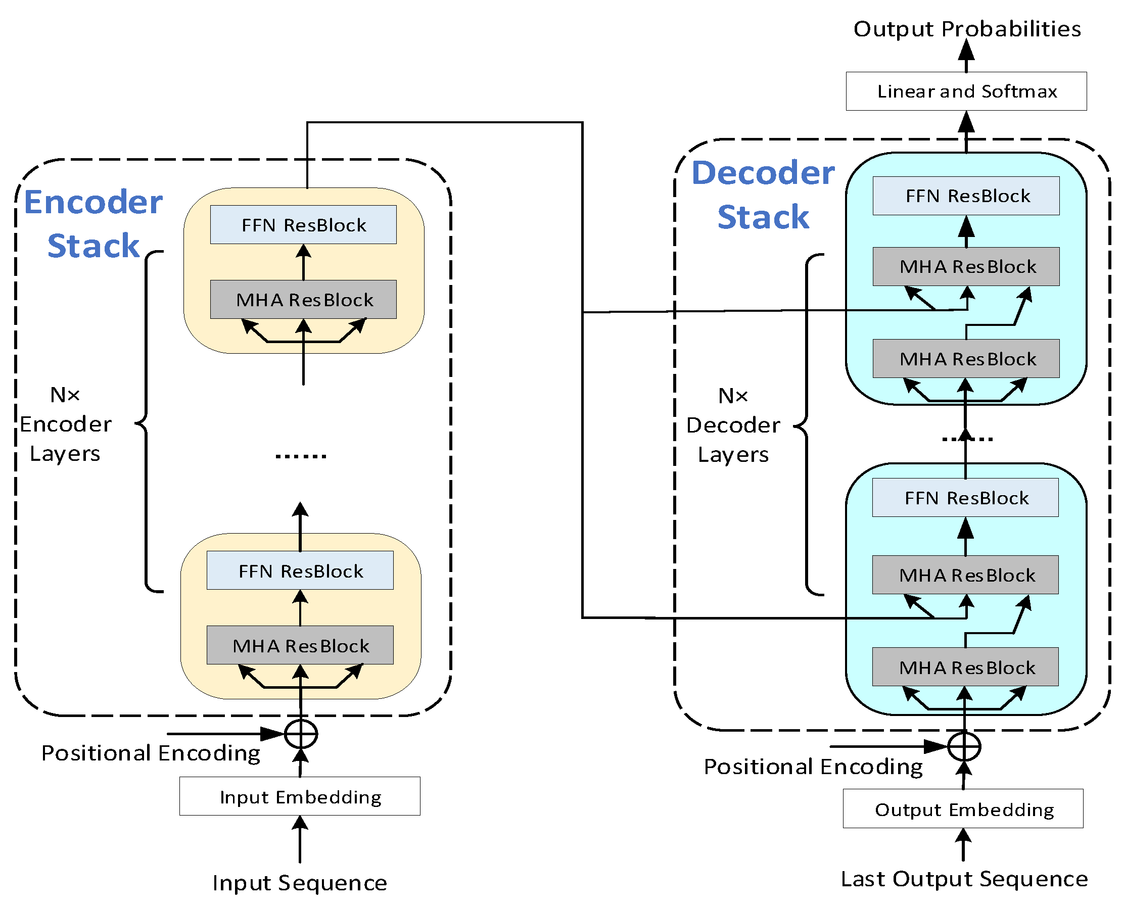
Figure 3 describes the model architecture of the Transformer in [13]. The encoder stack and decoder stack are two critical components with most of the trainable parameters and the most complex computations. The encoder layers and the decoder layers are composed of the multi-head attention (MHA) ResBlock and the position-wise feed-forward network (FFN) ResBlock.

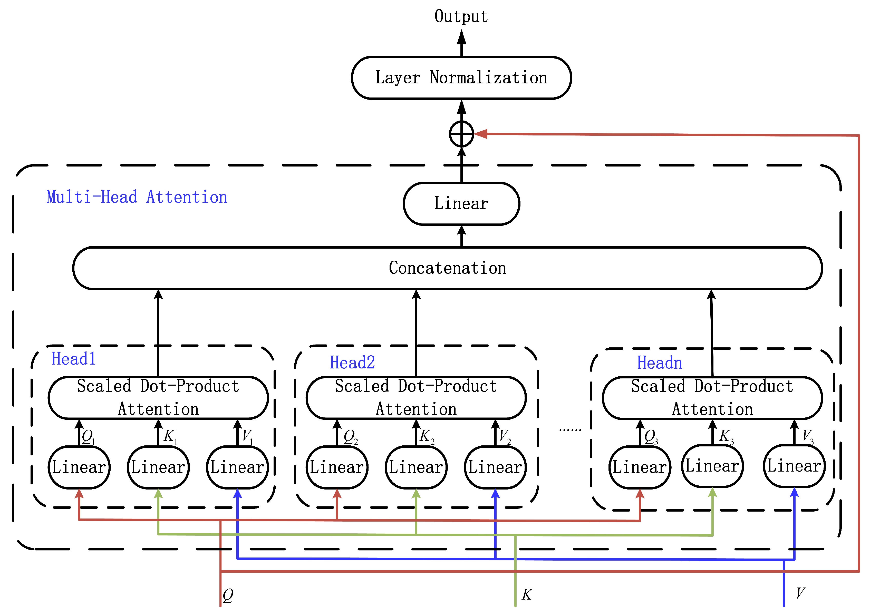
According to the description in [13], 1an MHA ResBlock has h Attention Heads. For each Head, the input is the same, including three tensors: Queries(Q), Keys(K), and values(V). Figure 4 shows the detail of the MHA ResBlock. The Attention function in the MHA of one Head can be expressed as follows:

$$Attention\left(Q_i,K_i,V_i\right)=softmax\left(Mask\left(\frac{Q_i{K}_i^T}{\sqrt{d_k}}\right)\right)V_i$$

(8)

The output tensors from different Heads are put together as tensor P. (9) represents the output of the MHA ResBlock:

$$\mathrm{MHA}\left(x\right)=LayerNorm\left(P{W}_G+x\right)$$

(9)

The FFN ResBlock is composed of two linear sublayers and a ReLU activation function between them. The output of this block is expressed as:

$$\mathrm{FFN}\left(x\right)=LayerNorm\left(x+ReLU\left(x{W}_1+b_1\right)W_2+b_2\right)$$

(10)

3. Proposed Cascade Neural Network

This section contains the main innovation of this work: a cascade neural network for LDPC coding recognition. In order to better present the proposed design, we firstly describe the system framework. Then, the CNN structure and the coding blind recognition network will be introduced, and their functions will be explained specifically.

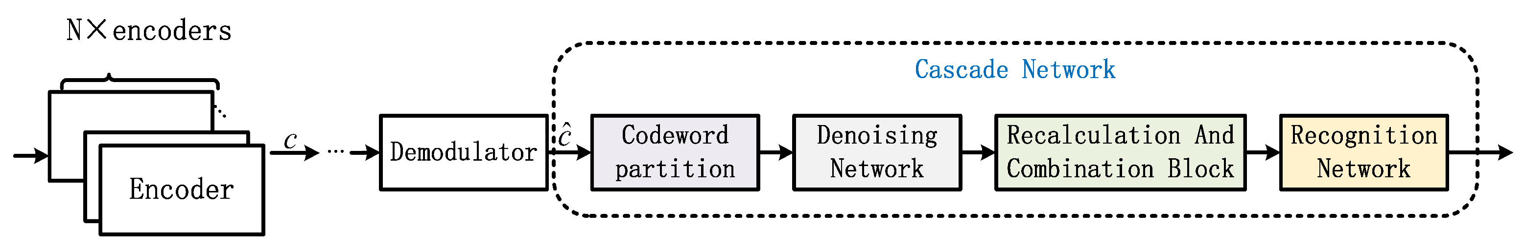
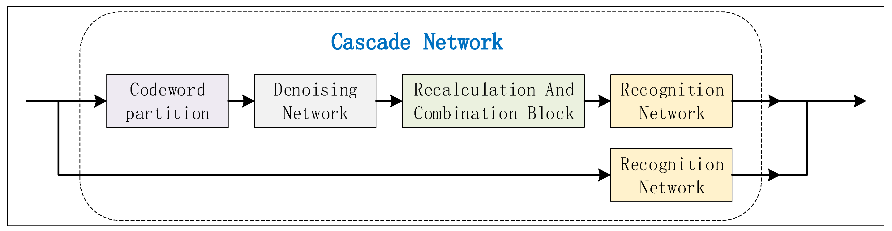
The input of the denoising CNN is a 1-D vector x, while the output vector is y. Both x and y are of size $\left(1,N\right)$. As shown in Figure 5, the received code words $\widehat{c}$ are uniformly distributed as N bits, and then sent into CNN. After denoising, y are used to recalculate $LLR$(L). $\widehat{L}$ denotes the concatenation of L with of size $\left(1,15N\right)$. The blind recognition network based on the Transformer takes $\widehat{L}$ as input. The output of the recognition network is the label, corresponding to the parity-check matrix H.

3.1. Denoising Networks

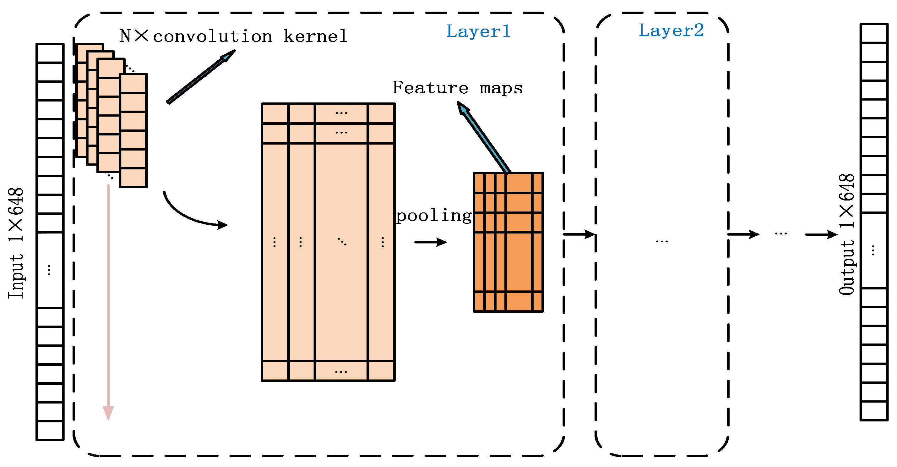
Figure 6 shows the denoising networks using CNN. The input of our networks is a 1-D vector. The feature map at the ith layer $o_i$ can be expressed in (11) as

$$o_{i,j}=ReLU\left(w_{i,j}\ast o_{i-1}+b_{i,j}\right)$$

(11)

where ∗ represents the convolution operation, and $w_{i,j}$ is the jth convolution kernel in layer i. $b_{i,j}$ represents the corresponding bias. The activation function is ReLU. In addition, the structure parameters of the proposed denoising network are given in

Table 1. The structure of the denoising network.

Layers	Numbers of Filters	Filter Size	Output Size
Conv2d1	64	(9, 1)	(128, 64, 648 )
Conv2d2-8	64	(9, 1)	(128, 64, 648)
Conv2d9	1	(9, 1)	(128, 1, 648)

.

In addition to the network framework, the loss function is also important for designing the network. It guides the training in the correct direction. $L_2$ loss, which is also called the mean squared error ($MSE$), is widely used in the area of image denoising. Suppose that $f\left(x\right)$ is the forward calculation output of the network, and y is the expected output. $L_2$ can be represented by

$$L_2=\frac{{\displaystyle \sum _{i=1}^n}{\left(f\left(x\right)-y\right)}^2}{n}$$

(12)

Inspired by the image denoising, $L2$ loss is also used in this design. Furthermore, in [22], the authors propose a method for recalculating the LLR. It obtains the empirical probability distribution function (EPDF) F of the residual noise through histogram statistics. In order to recalculate the LLR more easily, we consider that the residual noise preserves Gaussian distribution with various values of ${\widehat{\sigma }}^2$. Thus, $L_{\kappa }$ [25] is used to evaluate whether the residual noise meets Gaussian distribution. Residual noise is defined as $\tilde{n}$, and the numerical expectation as $E\left[\tilde{n}\right]$. $L_{\kappa }$ is expressed by:

$$\begin{array}{c}\hfill L_{\kappa }=\left(S^2+\frac{1}{4}{\left(C-3\right)}^2\right)\\ \hfill S=\frac{\frac{1}{D}{\sum }_{d=1}^D{\left({\tilde{n}}_d-E\left[\tilde{n}\right]\right)}^3}{{\left(\frac{1}{D}{\sum }_{d=1}^D{\left({\tilde{n}}_d-E\left[\tilde{n}\right]\right)}^2\right)}^{3/2}}\\ \hfill C=\frac{\frac{1}{D}{\sum }_{d=1}^D{\left({\tilde{n}}_d-E\left[\tilde{n}\right]\right)}^4}{{\left(\frac{1}{D}{\sum }_{d=1}^D{\left({\tilde{n}}_d-E\left[\tilde{n}\right]\right)}^2\right)}^2}\end{array}$$

(13)

S is called skewness, and C is called kurtosis. For a Guassian distribution, $S=0$, $C=3$. Thus, the loss function is

$$\mathsf{Ł}=\alpha L_2+\beta L_{\kappa }$$

(14)

where $\alpha +\beta =1$.

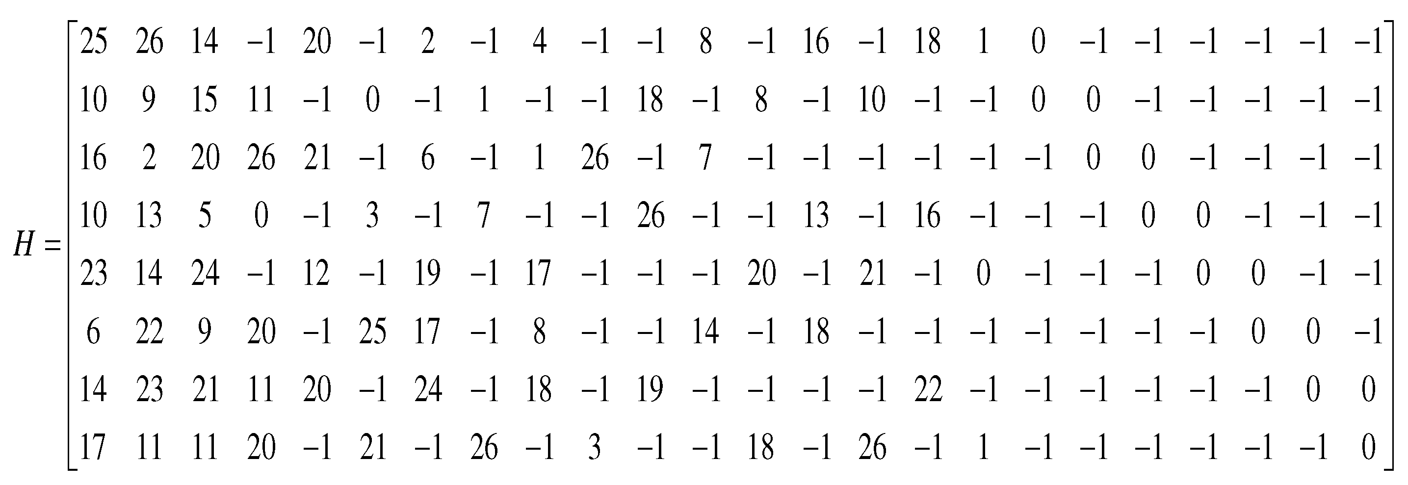
In this paper, the candidate sets of LDPC codes have the length $L=\left[648,1296,1944\right]$, and rate $R=\left[1/2,2/3,3/4,5/6\right]$. IEEE802.11 elaborates on these LDPC codes specifically, and is used for Wireless Fidelity(Wi-Fi). The H matrix of the LDPC code with $n=648$, $R=2/3$ is shown in Figure 7. The H matrix is constituted by two basic elements, i.e., a zero matrix represented by $-1$ and an identity matrix. The elements in the H matrix which are not equal to -1 represent the digits of rotating right of the identity matrix. In order to train denoising networks, we consider the AWGN with different SNR $S=\left[0,0.5,1,2,4,6,8\right] \mathrm{dB}$. Three code words $\left[c_1,c_2,c_3\right]$ with different lengths are sent to the channel. In order to prevent the dimension explosion of the neural network and reduce training time, the appropriate input size of the network is chosen, which is 648 bits. Thus, these code words are divided into 648 bits c, which is the shortest code word length. After the process of the sending end and channel, we get $\widehat{c}$ with white Gaussian noise added. Denoising networks use c and $\widehat{c}$ for training.

3.2. Recalculation of LLR

As mentioned in Section 3.1, the residual noise preserves the Gaussian distribution with various values of ${\widehat{\sigma }}^2$. It is easy to recalculate the $\widetilde{LLR}$:

$$\widetilde{LLR}=-2·\frac{\widehat{c}\left[i\right]}{{\widehat{\sigma }}^2}$$

(15)

3.3. Recognition Networks

After the above operation, the $\widetilde{LLR}$s are calculated at sizes of (1, 648). Then, 15 $\widetilde{LLR}$s are concatenated into 1-D data of size (1, 9720) defined as $I_R$, which is the input of the recognition network. However, because of the positional encoding layer in Transformer, the input of the network must be a fixed size. In order to identify these three different lengths of LDPC code and reduce the number of parameters, the ideas in the Swin Transformer are used in the recognition network.

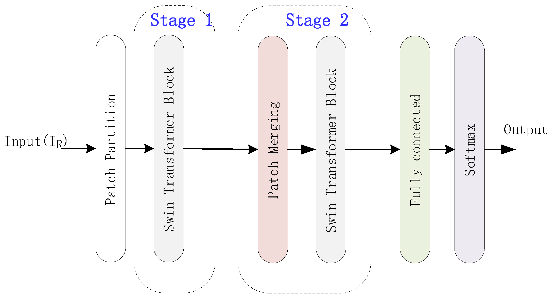
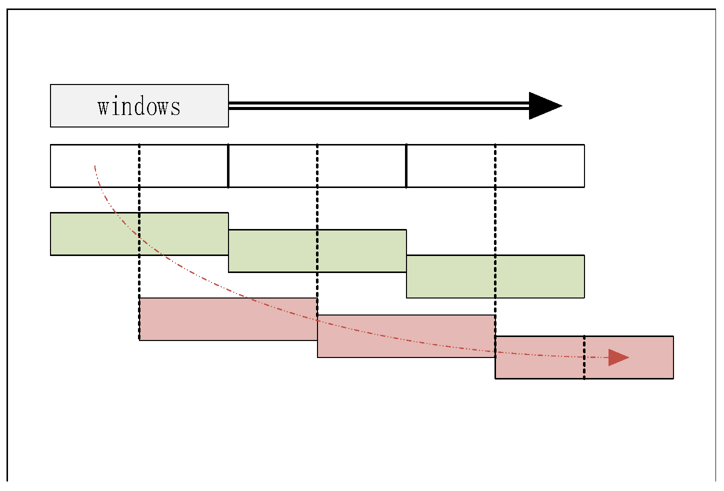
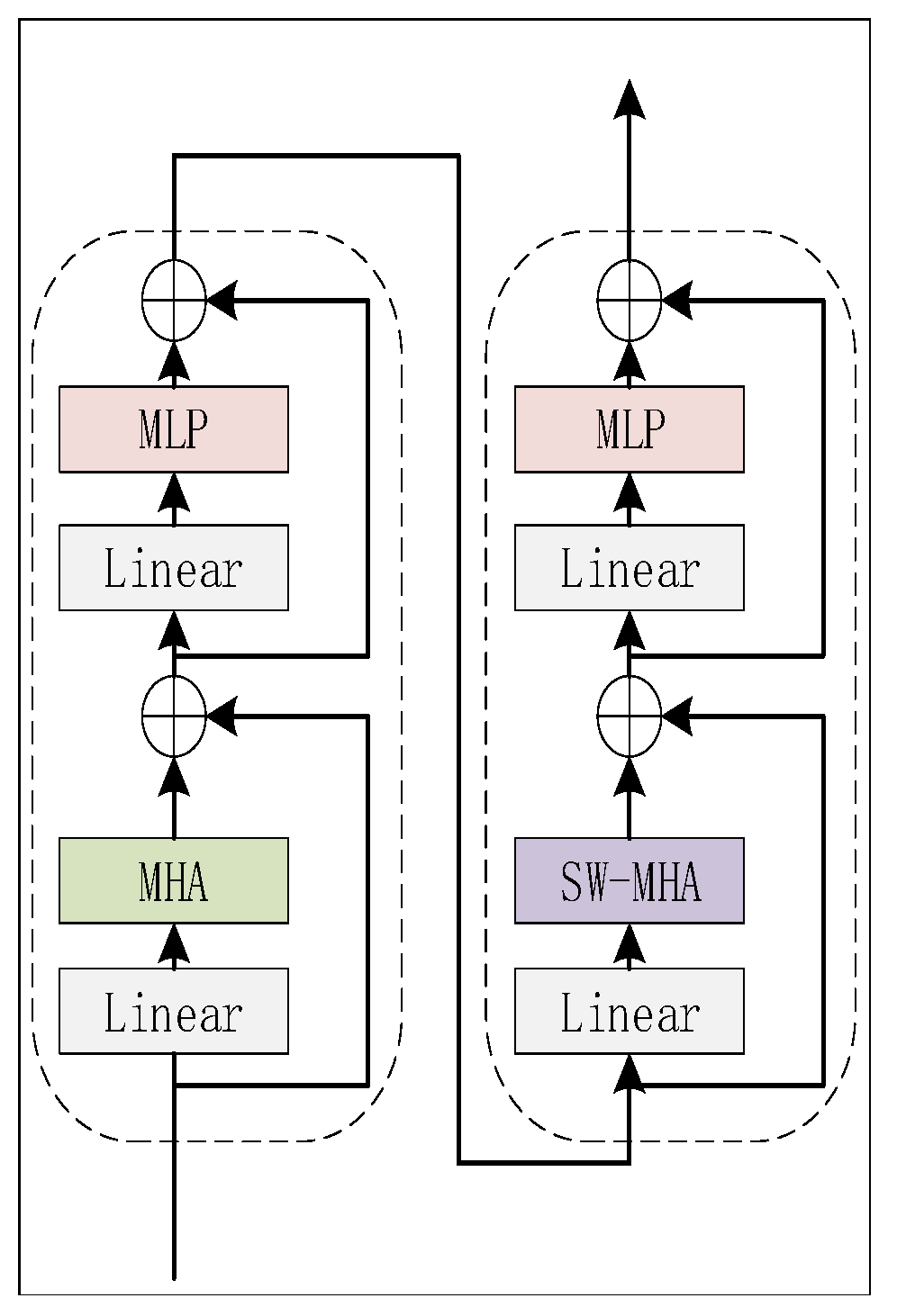
Figure 8 shows the architecture of the network. This network takes $I_R$ as input. Since the token size of this network is 324, $I_R$ is divided into 30 × 324 by Patch Partition layer. The window size is of 10 tokens and the relative position encoding (RPE) B is a learnable variable of size $\left(1,19\right)$. B is calculated by substituting its index into an RPE matrix of size $\left(1,19\right)$. The size of the RPE matrix is determined by the number of tokens in the window, and the relationship between tokens and windows is shown in Figure 9. The Swin Transformer Block contains two layers: one for MHA calculation, and another for shifted window MHA(SW-MHA) calculation. Figure 10 shows the detail of the Swin Transformer block. The window calculates MHA firstly, which is introduced in Section 2.3. In order to calculate SW-MHA, the feature map must shift circularly as shown in Figure 9. Then, the SW-MHA can be calculated the same way as the MHA.

It should be noted that the formula is a little different from (8) because of the difference in the strategy of linear embedding.

$$Attention\left(Q_i,K_i,V_i\right)=softmax\left(\frac{Q_i{K}_i^T}{\sqrt{d_k}}+B\right)V_i$$

(16)

B is the RPE mentioned before, and a mask is useless in this task.

The function of the patch merging layer is similar to the max-pooling layer in CNN, which is used to expand the receptive field. The vector size of stage 1’s output is the the same as its input with the size of $\left(30,324\right)$. Then, the outputs are resized into the size of $\left(10,324\right)$ by taking one of every three pieces of data from the output of stage 1. After a normalization in each row and a fully connected layer, the output becomes $\left(10,324\right)$. The Swin Transformer block in stage 2 is similar to stage 1. The difference is only the dimension, which is 10 in stage 2. Finally, the outputs of stage 2 of the size $\left(10,324\right)$ are sent to the fully connected layer and processed using the softmax function for classification.

There are three different types of datasets for the recognition network. The main difference between these three datasets is that the impact of noise on their data inside varies. The data in dataset 1 are noiseless, the data in dataset 2 are the output of the recalculation and combination block, which retain the residual noise, and the data in dataset 3 come directly from the demodulator without denoising. The label of these datasets is one-hot codes of 12 bits, which corresponds to each parity-check matrix H. The details of the datasets are given in

Table 2. The details of the datasets.

Attributes	Dataset 1	Dataset 2	Dataset 3
Numbers of H	12	12	12
SNRs for generation	∞	—	$\left[0,0.5,1,2,4,6,8\right]$
Modulation	BPSK	BPSK	BPSK
Numbers of training data	24,000	168,000	168,000
Numbers of validation data	7200	50,400	50,400
Whether channel soft information was used	-	YES	NO

. Each dataset included in Table 2 is randomly divided into 3 groups, i.e., the train set, validation set and test set. The train set accounts for $80\%$, while the validation set and test set account for $10\%$. Note that there is no other mechanism for accessing channel information, so dataset 1 and dataset 3 are sent to the network for training directly. The parameters of the recognition network are given in

Table 3. The parameters of the recognition network.

Layers	Input	Output	${\mathit{d}}_{\mathit{k}}$	Number of Heads
Patch Partition	$\left(128,1,9720\right)$	$\left(128,30,324\right)$	-	-
Swin Transformer Block	$\left(128,30,324\right)$	$\left(128,30,324\right)$	36	9
Patch Merging	$\left(128,30,324\right)$	$\left(128,10,324\right)$	-	-
Swin Transformer Block	$\left(128,10,324\right)$	$\left(128,10,324\right)$	36	9
Fully connected	$\left(128,10,324\right)$	$\left(128,12\right)$	-	-
Softmax	$\left(128,12\right)$	$\left(128,12\right)$	-	-

.

4. Experiment and Result

In this section, the function of the proposed network is verified in three steps. Firstly, the denoising network is trained and evaluated. Dataset 2 will also be built at this stage. Then, the datasets 1, 2, and 3 mentioned in Section 3.3 are used to train the recognition network respectively and evaluate the accuracy of this network. Finally, we analyse the cascade neural of the proposed network, and compare with the method in [7,16].

4.1. Denoising Network

As shown in Table 1, the batch size for training is 128. Furthermore, hyperparameters for training are given in

Table 4. Hyperparameters for training.

Optimizer	Initializer	Learning Rate	Stop Strategy
Adam	Kaiming	1e−4	Val loss not drop in 1e + 4 epoch

. The first-order moment estimation and second-order moment estimation of gradients are calculated using Adaptive Moment Estimation (Adam) to set the independent adaptive learning rates of different parameters. Kaiming initializers [26] are widely used in convolutional networks and perform well. After extensive experiments, we found that the convergence speed is the fastest when the learning rate is 1E-4, and the training will stop until the validation loss doesn’t drop in 1E+4 epochs.

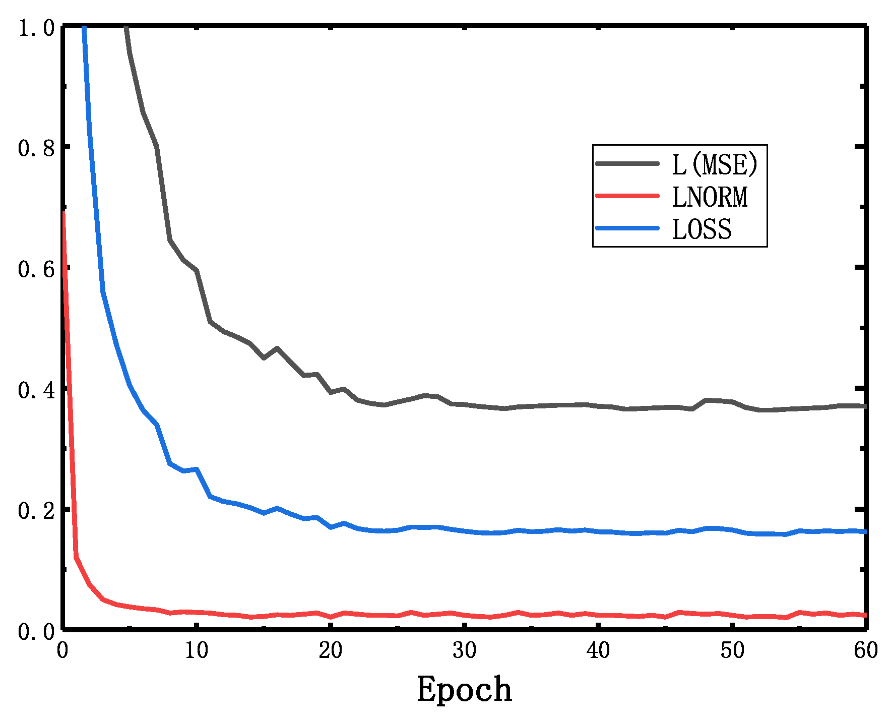
In order to intuitively demonstrate that if the function of this network is as expected, the loss functions will be $L_2$ and $L_{\kappa }$, this is shown in Figure 11.

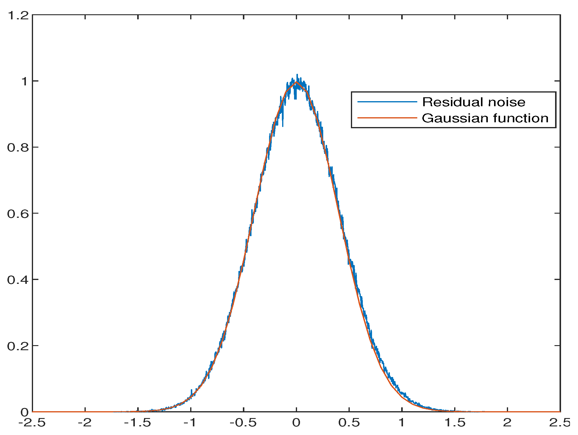
Moreover, the residual noise is exported and fitted to the Gaussian function in Figure 12. The blue line indicates the distribution of the residual noise from $-5$ dB to 5 dB, while the red one is the Gaussian fitting of these data. Both the Jarque-Bera test (JB-test) and Figure 12 indicate that the residual noise preserves the Gaussian distribution.

As mentioned in Section 3.3, dataset 2 is the output of this network with the corresponding labels. The variance $\widehat{\sigma }$ of the residual noise generated by the denoising network with different SNR inputs is counted, and the statistical results show that ${\widehat{\sigma }}^2$ is around 0.4, which means that the SNR of the output is about 4 dB, according to the formula below.

$$SNR=10lo{g}_{10}\left(\frac{1}{{\widehat{\sigma }}^2}\right)$$

(17)

It leads to good results when SNR is smaller than 4 dB. Even if the channel condition is good enough, this network can also provide approximate channel information, which can be used for the following work.

4.2. Recognition Network

Similar to the denoising network, the recognition network is trained using the three datasets mentioned above. The hyperparameters of these three networks are all the same, which are given in

Table 5. Hyperparameters for training.

Optimizer	Initializer	Learning Rate	Drop Out
Adam	Xavier	$0.001$ at the beginning; gradually decreased while training	0.5

. The Optimizer is the same as the denoising network, while the initializer used is Xavier, which initializes the mean value of the weights and bias to 0 and of various other values to 1. The learning rate is initially set to 0.001 and adjusted dynamically during training. In order to prevent overfitting, the drop out value we set is 0.5.

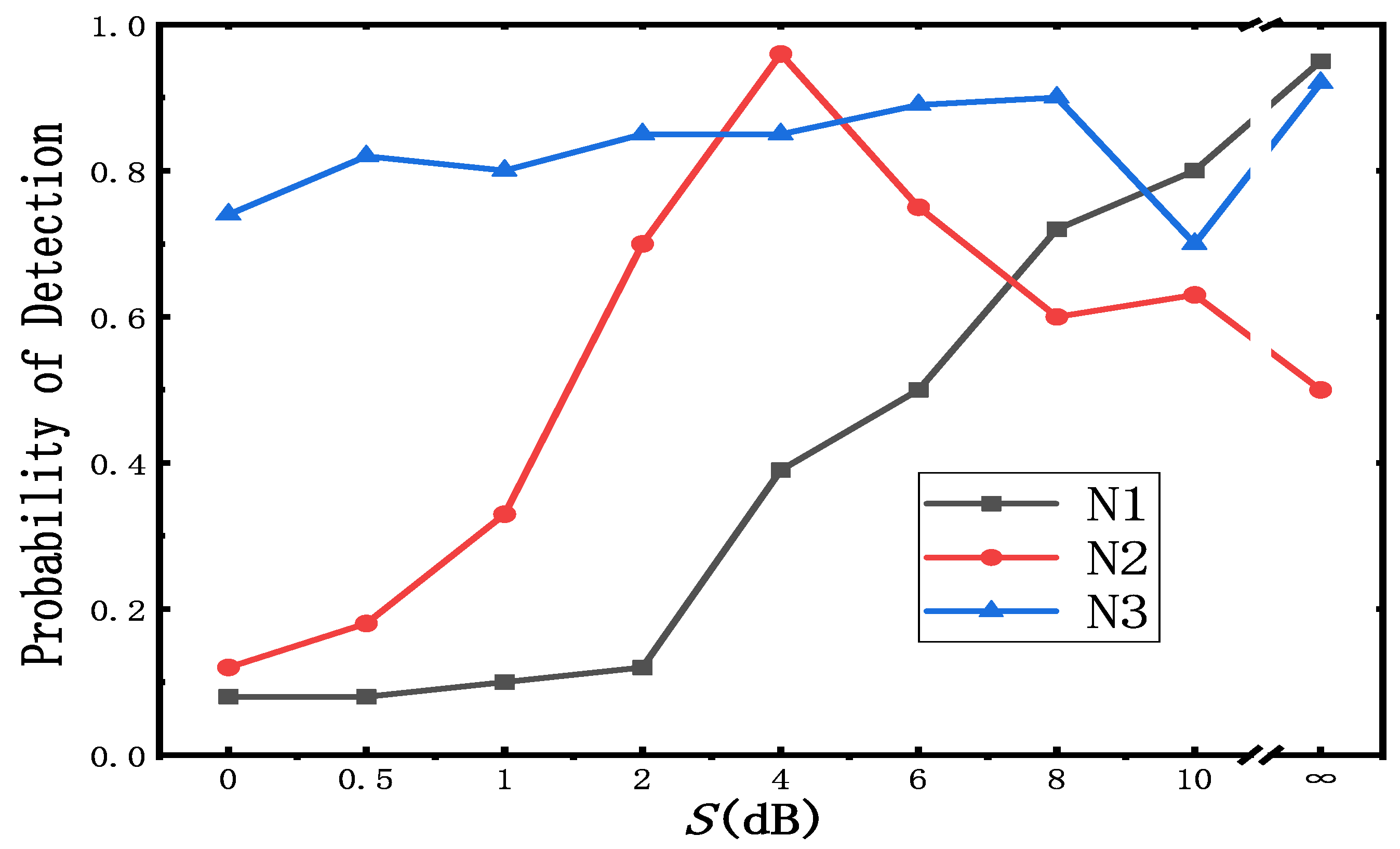
In order to verify the accuracy and robustness of the network, twelve types of LDPC codes with $\left[0,0.5,1,2,4,6,8,10,\infty \right]$ dB are used as the test sets. Figure 13 shows the performance of these three networks trained by different datasets.

$\left[N1,N2,N3\right]$ are the networks trained by $\left[dataset1,dataset2,dataset3\right]$, respectively, for convenience. As shown in Figure 13, $N1$ and $N2$ perform fairly well when the SNR(S) of the test set is the same as that of the training set. This network is robust, since it is able to recognize the LDPC codes with a SNR that has not appeared in the training set. However, the performance of $N1$ and $N2$ gradually deteriorates as the gap in the SNR between the test sets and training sets becomes larger. The accuracy of $N1$ is the worst when the S of the test set is 0 dB. On the contrary, $N3$ has more flexibility and is more adaptable to multiple situations due to the large variety of data in its training set. But it is less accurate than $N1$ and $N2$ for a particular SNR The above discussion shows that it is possible to obtain a highly accurate blind recognition network, as long as we ensure that the SNR deviation of the data after the denoising network is as small as possible.

Furthermore, it is noticeable that the accuracy is quite low when the S is less than 0.5 dB. We consider the trade-off of the accuracy and flexibility by rebuilding the dataset for the denoising network. The addition of new data with a low SNR will inevitably cause the degradation of denoising network performance, resulting in a decline in the accuracy of the recognition network. In order to improve the accuracy of the prediction of $\widehat{\sigma }$ from the denoising network, we rebuild datasets with a low SNR ([$-3,-2,-1,0,1,2,4$] dB) for the denoising network. After removing the low-SNR data, the recognition network using only high-SNR data can be further optimized. Hence, the proposed optimized structure is shown in Figure 14. The accuracy of this structure is shown in

Table 6. The accuracy of the optimized structure.

SNR$/\mathbf{dB}$	$-3$	$-2$	$-1$	0	1	2	4	6	8	10
Accuracy	0.866	0.871	0.895	0.920	0.925	0.951	0.911	0.874	0.862	0.867

. It is noteworthy that this system performs better with SNRs from $-3$ dB to 4 dB than with other SNRs due to the use of the channel information. Its accuracy is around $90\%$ when $-3$ dB ≤ S ≤ 4 dB, while the accuracy is around $87\%$ when 5 dB ≤ S ≤ 10 dB.

4.3. Experimental Setup

$P_d$ represents the probability of correct recognition, which can be described as

$$P_d=\frac{N_d}{N_t}$$

(18)

$N_d$ is the number of correctly recognized code words, and $N_t$ is the total number of the code words.

The method in [7] firstly estimates the signal amplitude and noise variance for the construction of the $LLR$s. It shows that $P_d$ is higher when they collect multiple blocks jointly for blind encoder identification. They assume that each encoder $\mathsf{\theta }$ lasts for M consecutive blocks. As the value of M increases, the reliability of the estimated LLR and the accuracy of blind recognition will be better. Since a test sample in datasets we built contains at least five consecutive code words, the $P_d$ for this network is compared with that of the method in [7] under the condition of $M=5$.

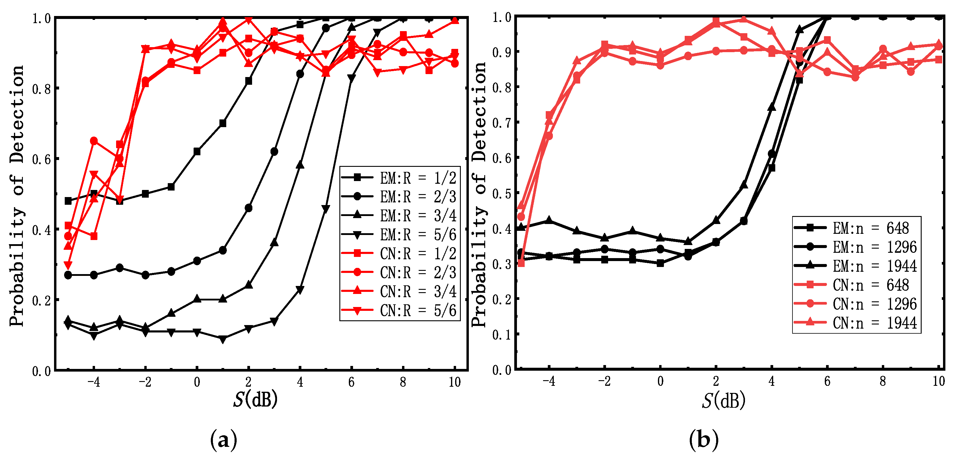
The $P_d$ for different code-rates$\left[1/2,2/3,3/4,5/6\right]$ is shown in Figure 15a, when the code word length is fixed at 648. Statistical methods are used in [7] for coding blind recognition. EM (expectation-maximization) represents the method in [7]. CN (cascade-network) represents the method we proposed. According to Figure 15a, the probability of detection increases as the code-rate becomes lower [7], while the $P_d$ of these four code words is mainly consistent using our method. In addition, it is easy to find that the method we proposed performs better when the S is between 0 dB and 5 dB. Although the accuracy of our method is not good enough when S is larger than 5 dB, it can also precisely recognize H in most cases.

In order to estimate $P_d$ for different code word lengths, the code-rates R are fixed at the same value of $5/6$. Figure 15b demonstrates the $P_d$ of these test samples. The overall trend of these curves is similar to that of Figure 15.

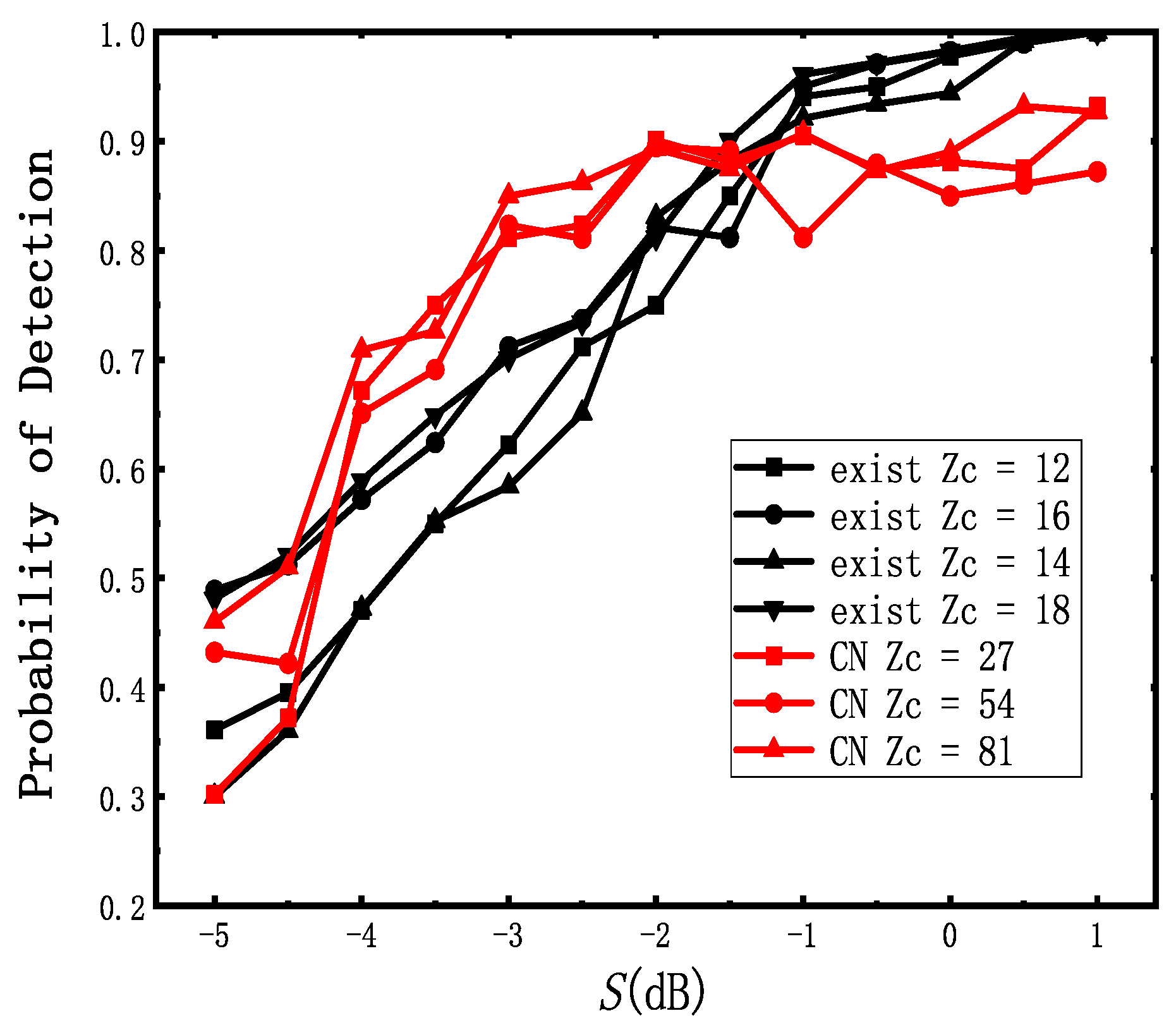
In addition to comparing with traditional blind recognition algorithms, another blind recognition method based on deep learning [16] is also compared. Figure 16 shows the accuracy of these two methods. Since the dataset mentioned in [16] is difficult to build, we can only roughly compare their accuracy. The results also show that our proposed network performs better when $-4$ dB ≤$S\le$$-2$ dB. Since our design does not need to generate $LLR$ information for each SNR, our network is more generic.

5. Conclusions and Discussion

In this paper, we proposed a cascade network structure for LDPC coding blind recognition. Compared with the traditional blind recognition algorithm, it performs better under the condition of low SNR.

The original intention of our design of the denoising network was to filter part of the noise and obtain the code word, which has residual noise in the Gaussian distribution. The results show that the denoising network can provide accurate channel information when the SNR gap in datasets is not large. In addition, it performs better when the SNR is small. For the recognition network, training for various different SNRs is not reliable. We prefer focalization training, which coincides with the function of the noise reduction network.

The generation matrix of LDPC codes in datasets is described in IEEE802.11n, which is widely used in short-range wireless communications technology. The proposed cascade network can identify the parity-check matrix of LDPC codes in datasets with a probability of $90\%$ when the S is larger than 0 dB. Furthermore, this network achieves about $80\%$ accuracy when the S is around $-2$ dB, which is better than other traditional methods.

After the division of the dataset and the optimization of the structure, this architecture performed better than the traditional method and another deep learning method. However, due to the limitation of the cascade structure, the training cost of the network is high, and the data division is also critical. Hence, the fusion of this structure and traditional algorithms may achieve better results. Here, we suppose a hypothetical structure with two different data paths, $PathA$ and $PathB$. The demodulated data is sent to two different data paths, and the final output is the one with higher confidence of these two data paths.

$PathA$ is for data with low SNR, while $PathB$ is on the contrary. Both paths have a recognition network, but the training sets of the two networks are different. Recognition networks on $PathA$ use the output of the denoising network for training. The datasets of the denoising network are of a low SNR, such as $\left[-5,-4,-3,-2,-1,0\right]$ dB or even lower, aimed to handle the situation of a bad channel condition. On the contrary, $PathB$ is for data with a high SNR. Firstly, the $LLR$ is evaluated blindly with the help of the traditional method. The soft information is subsequently used for training. Note that the recognition network can also be replaced by the traditional blind identification method, since the traditional method has already given good results when the SNR is high. At the end of these two paths, a discriminant function must be designed to determine whether the final output is from $PathA$ or $PathB$.

In short, our work confirmed that it is feasible to use the pure deep learning method for LDPC blind recognition, and that the performance is better after using the CNN for denoising. In the subsequent work, we will rebuild the dataset with a different channel condition and different parity check matrix of LDPC codes, which is widely used in modern communication, and verify the accuracy of the existing network on the rebuild dataset. In addition, the hardware acceleration architecture for the network is also being designed synchronously.

References

- Perrins, E. FEC systems for aeronautical telemetry. IEEE Trans. Aerosp. Electron. Syst. 2013, 49, 2340–2352. [Google Scholar] [CrossRef]
- Bonvard, A.; Houcke, S.; Marazin, M.; Gautier, R. Order statistics on minimal Euclidean distance for blind linear block code identification. In Proceedings of the 2018 IEEE International Conference on Communications (ICC), Kansas City, MO, USA, 20–24 May 2018; 2018; pp. 1–5. [Google Scholar]
- Yu, P.; Peng, H.; Li, J. On blind recognition of channel codes within a candidate set. IEEE Commun. Lett. 2016, 20, 736–739. [Google Scholar] [CrossRef]
- Gallager, R. Low-density parity-check codes. IRE Trans. Inf. Theory 1962, 8, 21–28. [Google Scholar] [CrossRef]
- Moosavi, R.; Larsson, E.G. Fast blind recognition of channel codes. IEEE Trans. Commun. 2014, 62, 1393–1405. [Google Scholar] [CrossRef]
- Xia, T.; Wu, H.-C. Blind identification of nonbinary LDPC codes using average LLR of syndrome a posteriori probability. IEEE Commun. Lett. 2013, 17, 1301–1304. [Google Scholar]
- Xia, T.; Wu, H.-C. Novel blind identification of LDPC codes using average LLR of syndrome a posteriori probability. IEEE Trans. Signal Process. 2014, 62, 632–640. [Google Scholar] [CrossRef]
- Wu, Z.; Zhang, L.; Zhong, Z.; Liu, R. Blind Recognition of LDPC Codes Over Candidate Set. IEEE Commun. Lett. 2020, 24, 11–14. [Google Scholar] [CrossRef]
- Valembois, A. Detection and Recognition of a Binary Linear Code. Discret. Appl. Math. 2001, 111, 199–218. [Google Scholar] [CrossRef]
- Cluzeau, M. Block Code Reconstruction Using Iterative Decoding Techniques. In Proceedings of the 2006 IEEE International Symposium on Information Theory, Seattle, WA, USA, 9–14 July 2006; pp. 2269–2273. [Google Scholar]
- Redmon, J.; Divvala, S.; Girshick, R.; Farhadi, A. You only look once: Unified, real time object detection. In Proceedings of the IEEE Conference on Computer Vision and Pattern Recognition (CVPR), Las Vegas, NV, USA, 27–30 June 2016; pp. 779–786. [Google Scholar]
- Young, T.; Hazarika, D.; Poria, S.; Cambria, E. Recent Trends in Deep Learning Based Natural Language Processing. IEEE Comput. Intell. Mag. 2018, 13, 55–75. [Google Scholar] [CrossRef]
- Vaswani, A.; Shazeer, N.; Parmar, N.; Uszkoreit, J.; Jones, L.; Gomez, A.N.; Kaiser, Ł.; Polosukhin, I. Attention is all you need. In Proceedings of the 31st International Conference on Neural Information Processing Systems, Long Beach, CA, USA, 4–9 December 2017; pp. 6000–6010. [Google Scholar]
- Shen, B.; Wu, H.; Huang, C. Blind Recognition of Channel Codes via Deep Learning. In Proceedings of the 2019 IEEE Global Conference on Signal, Information Processing (GlobalSIP), Ottawa, ON, Canada, 11–14 November 2019; pp. 1–5. [Google Scholar]
- Ni, Y.; Peng, S.; Zhou, L.; Yang, X. Blind Identification of LDPC Code Based on Deep Learning. In Proceedings of the 6th International Conference on Dependable Systems and Their Applications (DSA), Harbin, China, 3–6 January 2020; pp. 460–464. [Google Scholar]
- Li, L.; Huang, Z.; Liu, C.; Zhou, J.; Zhang, Y. Blind Recognition of LDPC Codes Using Convolutional Neural Networks. In Proceedings of the 2021 IEEE 4th International Conference on Electronics Technology (ICET), Chengdu, China, 7–10 May 2021; pp. 696–700. [Google Scholar]
- Chen, X.; Wang, X.; Zhao, H.; Fei, Z. Deep Learning-Based Joint Modulation and Coding Scheme Recognition for 5G New Radio Protocols. In Proceedings of the 2022 IEEE 22nd International Conference on Communication Technology (ICCT), Nanjing, China, 11–14 November 2022; pp. 1411–1416. [Google Scholar]
- Zhang, K.; Zuo, W.; Chen, Y.; Meng, D.; Zhang, L. Beyond a Gaussian Denoiser: Residual Learning of Deep CNN for Image Denoising. IEEE Trans. Image Process. 2017, 26, 3142–3155. [Google Scholar] [CrossRef] [PubMed]
- Zhang, K.; Zuo, W.; Zhang, L. FFDNet: Toward a Fast and Flexible Solution for CNN-Based Image Denoising. IEEE Trans. Image Process. 2018, 27, 4608–4622. [Google Scholar] [CrossRef] [PubMed]
- Guo, S.; Yan, Z.; Zhang, K.; Zuo, W.; Zhang, L. Toward Convolutional Blind Denoising of Real Photographs. In Proceedings of the 2019 IEEE/CVF Conference on Computer Vision and Pattern Recognition (CVPR), Long Beach, CA, USA, 15–20 June 2019; pp. 1712–1722. [Google Scholar]
- Liang, F.; Shen, C.; Wu, F. An Iterative BP-CNN Architecture for Channel Decoding. EEE J. Sel. Top. Signal Process. 2018, 12, 144–159. [Google Scholar] [CrossRef]
- Li, J.; Zhao, X.; Fan, J.; Shu, F.; Jin, S.; Qian, Y. A double-CNN BP decoder on fast fading channels using correlation information. In Proceedings of the 2019 IEEE/CIC International Conference on Communications in China (ICCC), Changchun, China, 11–13 August 2019; pp. 53–58. [Google Scholar]
- Gruber, T.; Cammerer, S.; Hoydis, J.; Brink, S.T. On deep learning based channel decoding. In Proceedings of the 2017 51st Annual Conference on Information Sciences and Systems (CISS), Baltimore, MD, USA, 22–24 March 2017. [Google Scholar]
- Lin, S.; Costello, D.J. Error Control Coding; Prentice-Hall: Hoboken, NJ, USA, 2007. [Google Scholar]
- Thadewald, T.; Büning, H. Jarque-Bera test and its competitors for testing normality: A power comparison. J. Appl. Stat. 2007, 34, 87–105. [Google Scholar] [CrossRef]
- He, K.; Zhang, X.; Ren, S.; Sun, J. Delving Deep into Rectifiers: Surpassing Human-Level Performance on ImageNet Classification. In Proceedings of the 2015 IEEE International Conference on Computer Vision (ICCV), Santiago, Chile, 7–13 December 2015; pp. 1026–1034. [Google Scholar]