Passive IoT Optical Fiber Sensor Network for Water Level Monitoring with Signal Processing of Feature Extraction

Abstract

This paper presents a real-time remote water level monitoring system based on dense wavelength division multiplexing (DWDM)-passive optical fiber sensor (OFS) network for the application of the Internet of Things (IoT). This network employs a broadband light source based on amplified spontaneous emission (ASE) as a seed light. This ASE light is spectrum-sliced by an athermal type arrayed waveguide grating (200 GHz × 16 channel), then distributed towards multiple sensing units (SU). Here, 16 SUs are installed vertically at the specified height in the water pool according to the design specification (i.e., spatial resolution). Then, each SU reflects an optical spectrum having a different reflection coefficient depending on the surrounding medium (e.g., air or water). By measuring these reflected optical spectra with an optical spectrum analyzer, the water level can be easily recognized in real time. However, as the sensing distance increases, system performance is severely degraded due to the Rayleigh Back-Scattering of the ASE light. As a result, the remote sensing capability is limited at a short distance (i.e., <10 km). To overcome this limitation, we propose a simple signal processing technique based on feature extraction of received optical spectra, which includes embedding a peak detection algorithm with a signal validation check. For the specific, the proposed signal processing performs the peak power detection, signal quality monitoring, and determination/display of the actual water level through three function modules, i.e., data save/load module, signal processing module, and Human–Machine Interface display module. In particular, the signal quality of the remote sensing network can be easily monitored through several factors, such as the number of spectral peaks, the wavelength spacing between neighboring peaks and the pattern of detected peak power. Moreover, by using this validation check algorithm, it is also possible to diagnose various error types (such as peak detection error, loss of data and so on) according to the pattern of measured optical spectra. As a result, the IoT sensor network can recognize 17 different level statuses for the water level measurement from a distance of about 25 km away without active devices such as optical amplifiers (i.e., passive remote sensing).

1. Introduction

Optical fiber sensor networks (OFSNs) are actively utilized in many industrial fields, especially for monitoring applications, including hot spots for electrical power cables, external intrusion, railways, structural health, etc. [1,2,3,4,5]. This is due to the distinctive advantages of OFS, such as a passive-remote sensing characteristic, tolerance to electromagnetic interference, radiation resistance, redundancy, etc. [6,7]. Moreover, various multiplexing techniques make it possible to enhance the system performance (e.g., sensing distance and spatial resolutions) as compared to traditional electrical sensors [8,9,10]. Among those advantages, passive/remote sensing features are becoming more and more important with the emergence of the Internet of Things (IoT).

IoT is a cloud of interconnected physical devices (such as a massive number of sensors and actuators, gateways, data servers, etc.) for data acquisition, processing and analysis [11,12]. The architecture of an IoT-based sensor network can be broken down into four different layers: (i) the Sensing layer (sensor node) composed of sensors and/or actuators for monitoring or controlling the environmental conditions; (ii) the Network layer, including the transmission channel for measurement and/or control of data (via wireless or wired media) and gateway for data conversion/extraction/acquisition, (iii) Service layer (or Data center) performing data analysis, management, and secure storage for user solutions, and (iv) Application layer based on user interface for various applications (e.g., smart home/factory/transportation, health care, agriculture, etc.), as summarized in Figure 1.

Most IoT-based sensor networks employ wireless sensors and/or actuators to monitor or control environmental conditions [13,14,15,16,17,18,19,20]. However, typical wireless sensor networks (WSNs) require an electrical power supply to sensing nodes, which would be a great challenge. This is because wireless IoT devices are normally powered by primary batteries that need to be installed at remote locations [15]. Although the batteries have a high energy density, they have a limited lifetime. Hence, it causes maintenance issues that are closely related to operating expenditures (OPEX). Furthermore, battery replacement on a regular basis is not desirable for sensor networks in extremely harsh environments such as nuclear power plants. As an alternative solution, the power-over-fiber (PoF) technology has been proposed, which can optically supply electrical power to the wireless sensing node via a photovoltaic power converter [21,22,23,24]. This technique has been improved significantly with the advance of photonics components since it was first reported in 1978 [25]. As a result, it has been employed in a wide range of applications such as electrical, wireless communication, safety and so on [26,27,28]. However, this technology requires expensive high-powered lasers that are difficult to manipulate and manage. In addition, it is difficult for a single laser to provide enough power to multiple sensing units simultaneously, and transmission distances for optical power delivery are limited to a few hundred meters.

Recently, we proposed a simple passive optical fiber sensor network (OFSN) for the application of water level monitoring in a nuclear power plant (NPP). This sensor network can provide good performance at remote sensing distances (more than a few km) and high spatial resolutions (less than tens of cm) without directly providing electrical power to the sensing node [29,30]. Moreover, it does not need a photovoltaic power converter that converts optical power to electrical power for the sensors and/or actuators. For the specific, the proposed OFSN employs amplified spontaneous emission (ASE) as a seed light source at the monitoring station and an athermal type arrayed waveguide grating (AWG) as a (de-)multiplexer at the remote node. These components play a key role in the implementation of dense wavelength division multiplexing (DWDM) and make it possible to monitor the reflected optical spectra depending on the water level of the spent fuel pool (SFP) in the NPP. It subsequently offers a passive characteristic with low insertion losses as well as a simple architecture that allows for an intuitive analysis process and robustness to environment changes (e.g., temperature). However, the remote sensing capability can be severely reduced due to the Rayleigh Back-Scattering (RBS) light generated by the ASE, which is launched at the monitoring station. As a result, the sensing distance was limited to 10 km when the water level was distinguished by human eyes.

In this paper, we demonstrate a passive IoT optical fiber sensor network based on the DWDM scheme. Specifically, we investigate the passive remote sensing capability for water-level measurement with a signal processing technique based on feature extraction from the received optical signal. This signal processing technique employing a peak detection algorithm features fast processing and simplicity to determine the water level and its validity. The demonstration results show that it is possible to effectively detect actual water levels according to the reflected optical spectra via a user interface display system. It allows the proposed IoT sensor network to recognize 17 different level statuses for the water level measurement from a distance of about 25 km away without active devices such as optical amplifiers (i.e., passive remote sensing).

2. Architecture of Passive IoT Optical Fiber Sensor Network for Water Level Monitoring

As shown in Figure 2, the passive IoT optical fiber sensor network comprises four function blocks: (1) monitoring station (Main Control Room or Emergency Operation Facility); (2) transmission channel (single-mode fiber, SMF); (3) remote node (Equipment room); and (4) multiple SUs in the SFP.

The monitoring station includes a reflectometer and data server system. First, the reflectometer includes a Broadband Light Source (BLS) based on ASE light for seeding to the network (fiber to SUs), an optical spectrum analyzer (OSA) for measurement of the reflected optical signal with Analog-to-Digital (A/D) conversion and an optical circulator (OC) for separation between transmission and detection part. The BLS is an optically pumped erbium-doped fiber amplifier (EDFA) that generates a large bandwidth and gain-flattened ASE light. Second, the data server system consists of a central server and a user server. The central server is not only a database (DB) for the collection of data but also a processor/analyzer to determine the water level from the received digital data (i.e., reflected channel spectra). Then, the processed/analyzed data is sent to the user server to display the actual water level of the SFP and the integrity of acquired data on the User-Interface monitor. We employed the SMF as a transmission channel; this distance could be tens of kilometers. The AWG at the remote node distributes the spectrum-sliced ASE light to the SUs (i.e., de-multiplexes) and combines the signals from multiple SUs (i.e., multiplexes), with each SU representing the current water level. Each SU is a fiber-optic connector, and a portion of the spectrum-sliced ASE light is reflected back to the monitoring station due to the Fresnel reflection. It is worth noting that the various types of fiber-optic connectors can be considered according to the circumstances [8].

3. Water Level Measurement with Signal Processing Technique

3.1. Basic Measurement Principle

The basic principle of water level measurement is based on the Fresnel reflection from the end facet of each SU placed in a pool of water at a specific height. Changes in the medium surrounding the SU induce changes in the reflected optical power, and the related Fresnel coefficients for the air ($R_a$) and for the water ($R_w$) are represented as [31]:

$$R_a={\left(\frac{n_f-n_a}{n_f+n_a}\right)}^2 , R_w={\left(\frac{n_f-n_w}{n_f+n_w}\right)}^2$$

(1)

where $n_f$, $n_a$, and $n_w$ are the refractive indices of the optical fiber (1.449), the air (1.000), and the water (1.315, 10 $℃$), respectively [30]. These values are considered to be constant because they have wavelength/temperature-independent characteristics within C-band [29]. The calculated Fresnel reflections $R_a$ and $R_w$ are −14.7 dB (3.36%) and −26.3 dB (0.23%), respectively, as a result, they have a power difference ratio (e.g., $R_a-R_w$) of 11.6 dB. It is worth noting that this power difference ratio corresponds to the peak power difference of two distinct cases (i.e., air vs. water) without consideration of the background noise. Here, we define the spectral peak power difference as extinction ratio ($ER$) in the dB scale, as shown below.

$$ER\left(\lambda \right) \left[dB\right]=10·log{\left[\frac{R_a\left(\lambda \right)}{R_w\left(\lambda \right)}\right]}_{Max}$$

(2)

However, the fiber-optic system could suffer from undesirable back-reflections and optical crosstalks from passive devices, connectors, fiber splice points, etc. It results in the rise of the background noise, decreasing the peak power difference ratio (i.e., $ER$).

We already verified the theory by comparing it to experiments as well as simulations in [30]. Figure 3a shows the measured (red dotted lines) and simulated (solid black lines) optical spectra of the reflected optical signals by the SU where it is in the air and water, respectively. The value of $ER$ (i.e., the maximum peak power difference) was about 10.6 dB. Due to the background noise, this value was 1 dB smaller than the predicted value using Equation (1). Then, we investigate the impact of background noise on the$ER$, as shown in Figure 3b. Both the peaks of $I_a$ and $I_w$ slightly increase with the background noise power, and this trend is more pronounced for $I_w$ than $I_a$. As a result, the value of $ER$ decreases as background noise increases.

3.2. Multi-Channel Sensing with System Performance Indication (SPI) Parameter

For the multi-channel (multi-level) sensing capability, we exploit a passive DWDM technique (BLS + athermal AWG) in the IoT-based optical fiber sensor network. In this section, we experimentally demonstrate the proposed sensor network in a back-to-back condition and compare it with theoretical predictions in order to check the feasibility of multi-channel sensing.

As shown in Figure 4, the experimental setup included the C-band BLS (LiComm, OFB-ACB) that generated ASE light (bandwidth > 32 nm and flatness < 1.5 dB). The optical power of ASE light at the input of AWG was about 14.1 dBm after passing through the optical circulator with an insertion loss of 0.8 dB. To monitor the outpower of BLS, we inserted a 99:1 optical coupler and optical power meter (Thorlabs, PM20) between the BLS and the optical circulator. In addition, for implementation of the passive DWDM, we used the fiberized flat-top type athermal AWG (ANDevices) that has 16 channels on ITU-T DWDM grid with a channel spacing of 1.6 nm and 3-dB bandwidth of 1.03 nm, respectively, accommodating up to 16 SUs. Here, the SUs indicate the fiber-optic connectors installed at the output fibers of the AWG. We particularly used the standard LC/PC type connectors to minimize the surface tension of the water at the end of the connector surface. By installing 16 SUs at different heights with an even spacing inside the pool, we could distinguish the water level with 17 different steps (0 to 16 steps). Here, the number of SUs is closely related to the spatial resolution of the measurement system. In this system, the spatial resolution ($h$) can be defined as the below equation,

$$h=H/\left(N+1\right)$$

(3)

where $H$ is the total height of the pool to be measured, and $N$ is the number of SU. For example, for the 3.4 m depth of the water pool, the spatial resolution becomes 0.2 m with the 16-channel AWG.

At the receiving side of the monitoring station, we utilized an OSA (Yokogawa, AQ6370D) to measure the optical spectra from 1530 to 1565 nm at the C-band. These measured data (wavelength & optical power) were periodically transmitted to the central/user server via general purpose interface bus (GPIB), i.e., IEEE 488. It is worth noting that the low insertion loss of the AWG (i.e., <3.5 dB) leads to improved dynamic range as compared to the system using optical splitters [32].

Figure 5a,b show the measurement and simulation results of the optical spectra at the half-full water level, respectively. The experimental result shows a good agreement with the simulation. The value of $ER$, which is a system performance indicator, was about 10.6 dB. This parameter ($ER$) may have to be degraded as the remote sensing distance increases because of the RBS of transmitted BLS light. Thus, it is imperative to determine the lower bound of $ER$ to secure the reliability of the sensing network. The actual value of $ER$ can be misread by multiple factors. Firstly, the received optical power can be varied by about 0.8 dB over the C-band due to the temperature variation (10–100 $℃$) in the water pool. The simulation results are shown in the inset of Figure 5b by assuming that the reflective indices of water are 1.312 at 40 $℃$, 1.306 at 70 $℃$, and 1.298 at 100 $℃$, respectively [33]. This is because the environmental (e.g., temperature) variations in the pool mainly cause the index change of the water, and it eventually results in the change of the optical power reflected by the SUs (i.e., peak power increase) [29]. It is worth mentioning that we employed an athermal AWG to implement a passive remote sensing system based on DWDM, thus having no impacts on crucial system parameters such as the peak numbers and channel spacing. In addition, the un-flatness of the BLS output spectrum (1.5 dB) and insertion loss deviation among channels of AWG and SUs (<1 dB) can affect the received optical power too. Therefore, the $ER$ is supposed to be maintained around 3 dB to ensure the correct measurement and determination. It should be noted that this minimum $ER$ value can be decreased with high-quality low-loss passive optical components.

3.3. Level Determination with Signal Processing Technique Based on Feature Extraction

In the proposed system, post-signal processing is crucial to determine the water level from the received data. It could be done through the observation of optical spectrum by operators or technicians, though it is not only inefficient but also unreliable, especially on a long-term basis. However, this problem will be even more intense when the number of SUs is increased to enhance the spatial resolution. It should be noted that the spatial resolution can be easily increased by utilizing another wavelength band of BLS with a cyclic characteristic of AWG [34] and/or reducing the channel bandwidth of AWG [35]. Hence, we introduce a signal processing technique based on feature extraction from the received optical signal. The proposed signal processing performs the peak power detection and signals quality monitoring through 3 function modules, i.e., a data save/load module, a signal processing module, and Human–Machine Interface (HMI) display module, as described in the flow chart, Figure 6.

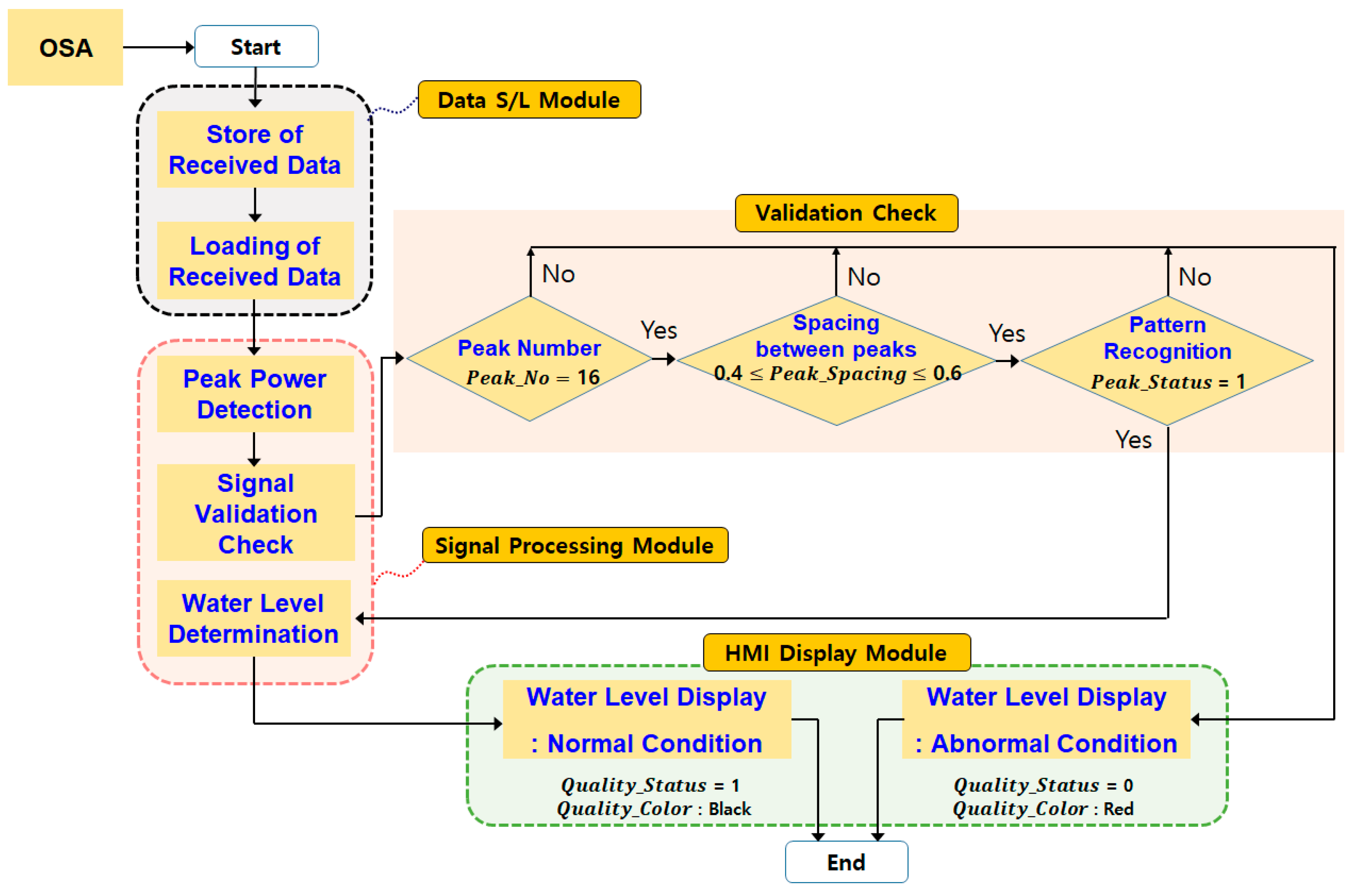
• Data Save/Load Module: This module brings the received raw data from OSA to the DB in the central server, where data are represented by [501 × 2] matrix for wavelength (the first column) and measured optical power (the second column). After converting the shape of the matrix from [501 × 2] to [2 × 501], the data is sent to the signal processing module to find out the peak power and its corresponding wavelength of each SU.
• Signal Processing Module: This module consists of three function blocks: (i) peak detection, (ii) signal validation check and (iii) water level determination. The first function block finds out the peak power and wavelength of each SU channel from the data matrix. Then, the quality of the signal (QoS) is evaluated by the signal validation block to check on the integrity of the received data. In particular, this validation process monitors several factors, such as the number of peak powers ($Peak\_No$), the wavelength spacing between neighboring peaks ($Peak\_Spacing$) and the pattern of detected peak power ($Peak\_Status$). Based on these parameters, the quality status variable ($Quality\_Status$) is set to “1” (normal status) or “0” (abnormal status). In addition, the text color ($Quality\_Color$) for the status panel is also set to black in normal conditions or red in abnormal conditions. Finally, if the signal quality is turned out to be normal status, the actual water level is determined by the function block of water level determination. This determination process is proceeded by comparing the pre-set decision level (DL) with the detected channel peak powers (i.e., “1” when DL > channel peak power, and “0” when DL ≤ channel peak power). Then, using the signal pattern (e.g., “0000 0000 1111 1111” for a half-full water pool), the water level is determined and displayed.
• HMI Display Module: The signal processing results are delivered to the DB of the user application server for the display by the HMI display module. It shows diverse information such as the measured spectrum, the peak positions, the monitored water level, the pre-set decision level, the status panel to describe the signal quality condition, and so on. The details of the HMI display will be explained in Section 4.2.

Figure 7 shows the signal processing results of three different cases: (a) almost empty, (b) half-full, and (c) full water level, respectively, where the peak position of each channel is marked with the red triangle (▲). The pattern of spectral peaks (related to $Peak\_Status$) did not show any abnormality, indicating the measurement result is reliable (i.e., $Quality\_Status$ = 1). To be specific, the total number of peaks detected ($Peak\_No$) was 16, and the wavelength spacing between each neighboring peak power ($Peak\_Spacing$) are positioned between 0.4 and 0.6 nm. Note that those parameters can alter depending on the system design coefficients, such as the number of AWG channels, the optical bandwidth of each channel, and its spectral shape.

4. Passive Remote-Sensing Capability with Signal Processing Technique

4.1. Back-Scattering Induced Degradation of Remote Sensing Capability

As mentioned in the previous sections, randomly-distributed variations in the refractive index of the silica fiber generate RBS as well as attenuation [30]. This results in the degradation of the remote sensing performance. To investigate this RBS effect, we measured the optical spectra depending on the sensing distance. In this experiment, we employed the standard SMF with a loss of 0.22 dB/km.

Figure 8a–d represents the measured optical spectra in the cases of lowest, half and fullest water levels at four different distances (10 km, 20 km, 25 km and 30 km), respectively. It shows the background noise level increases (i.e., $ER$ decreases) as the sensing distance increases because of the RBS. In particular, the level of signal “0” (=SUs submerged) becomes comparable to the RBS-induced background noise at 10 km already. Thus, according to the conventional decision process, the achievable sensing distance is limited to 10 km or less. However, it is still possible to recognize the spectral peaks and their optical power up to 25 km by adopting the proposed signal processing procedure. Moreover, the value of $ER$ is still 3 dB or larger, meeting the minimum margin requirement so as to guarantee the correct water-level determination, as previously discussed in Section 3.2. It implies that the proposed IoT sensor network can operate up to 25 km without considering any power supply issues in the remote local field.

For the sensing distance of 30 km (as shown in Figure 8d), the RBS and fiber-induced signal attenuation decreased the value of $ER$ to 1.6 dB, resulting in peak-detection errors and loss of data (see blue and orange circles). The loss of data is supposed to occur when the measured peak power is equal to or lower than the background noise power. As a result, the peak power detection algorithm could not find out the peak power within the specified wavelength range per SU channel (i.e., $Peak\_Spacing$). The peak power detection error is similar to the loss of data, except that the measured peak power is slightly higher than the background noise power, which induces the detection of more than one peak power and/or incorrect peak power position. These errors can be easily detected by the signal validation check algorithm in the signal processing module. In contrast to the experiment result, there was no error detected in the simulation with a sensing distance of 30 km. This is attributed to various factors, such as the flatness of the BLS output spectrum, the deviation of insertion losses among AWG channels/SUs, etc.

4.2. Full Demonstration of Remote Sensing with a Human–Machine Interface Display Module

This section gives explanations of the HMI display in detail, as illustrated in Figure 9. The HMI display module consists of four parts, i.e., (a) optical spectrum monitoring window, (b) water level indicating bar, (c) status panel (text box), and (d) start/stop buttons. The specific functions are explained as follows. It takes less than 1 s for data to load and show on the monitor, and thus it is possible to monitor the water level of remote locations on a real-time basis.

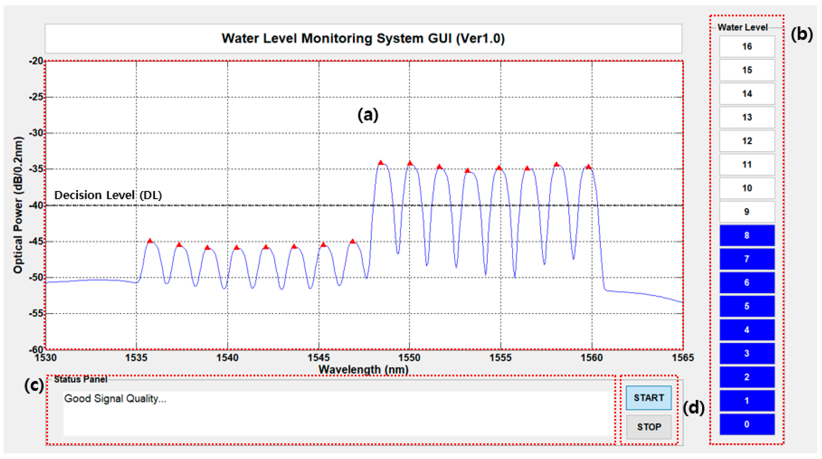
• Spectrum display window: This window shows the measured optical spectrum, which is saved in the DB of the central server. The result of the peak power detection is also displayed with red solid triangle marks on the displayed optical spectrum. Moreover, the decision level is represented with a black dashed line (---) for the determination of the water level. Below this level, the SUs are considered to be in the water, and vice versa.
• Water level indicating bar: This bar represents the actual water level measured, which is directly converted from the measured optical spectrum. A total of 17 steps of water levels can be represented according to the measurement of the water level (Step 0~16).
• Status panel: The signal validation results are shown on this panel. It contains information on signal conditions based on the measured optical spectrum using different text colors. If the measured optical signal is in good condition, the text is displayed in black; otherwise, the color of the text is changed to red.
• Start/Stop buttons: The real-time information shown on the monitor is updated every second after the start button is pushed. If the stop button is selected, the update is paused.

Based on the HMI Display Module, we fully demonstrated the IoT optical fiber sensor network for monitoring the water level at a distance of 25 km. Figure 10 shows the captured HMI displays for two different cases: (a) normal and (b) abnormal operations. The decision level was set to be −42.05 dBm/0.2 nm to distinguish two different levels (i.e., “0” and “1”) for both cases. Figure 10a shows the result of half water level detection in normal operation. The water level indicating graph bar correctly presents the actual water level from the measured optical spectrum with a proper message on the status panel. On the other hand, Figure 10b shows an example of abnormal operations of the sensor network in which the quality of the received optical signal did not meet the requirement, resulting in the loss of data and peak power detection error. This type of error typically occurs due to the physical damage of SUs and/or related AWG channels. As a result, the system is put on alert with the color of the water level bar changed to red and the error message shown up on the status panel.

5. Conclusions

This paper proposed and demonstrated an optical fiber sensor network integrated with an IoT-based signal gathering and processing technique for monitoring the water level of the spent fuel pool in nuclear power plants. Unlike conventional wireless IoT sensor networks, the proposed technology made use of fiberized optical components and DWDM so as to improve the sensing distance and resolution. Moreover, the passive characteristics of the proposed system utterly eliminated the necessity of power supply to remote locations. This IoT sensor network particularly utilized a BLS based on ASE as a seeding light source at the monitoring station. The launched BLS light was spectrum-sliced and distributed by an AWG towards multiple SUs that were installed at different heights in the water pool vertically. Each SU reflected the optical signal at a different ratio (i.e., $ER$) according to the surrounding medium (“1” with SU in the air vs. “0” with SU submerged) back to the monitoring station. Although the water level could be determined with the help of OSA, the sensing distance was limited to less than 10 km, partly due to the RBS of the seeded ASE light. Furthermore, it did not have the post signal processing algorithms for automation. To overcome these limitations, a simple signal processing technique based on feature extraction was applied to the sensor network. This technique could enhance the efficiency of the system and also increase the sensing distance up to 25 km without any optical amplification.

On the other hand, the system performance could be degraded (i.e., a decrease of $ER$ or loss of data) due to the floating or small particles in the water pool. Because the selected sensing units are a type of contact sensor, it may be possible to cause staining on the surfaces of the sensing units with these particles. However, in nuclear power plants, this can be considerably mitigated by the purification system of the spent fuel pool. This purification function is usually carried out through one or two flow paths to prevent the corrosion of spent fuels and related facilities [30]. In addition, maintenance activities (e.g., a periodic performance testing) help to monitor the condition of the sensing units.

References

1. Allwood, G.; Wild, G.; Hinckley, S. Optical fiber sensors in physical intrusion detection systems: A review. IEEE Sens. J. 2016, 16, 5497–5509. [Google Scholar] [CrossRef] [Green Version]
2. Wei, C.-L.; Lai, C.-C.; Liu, S.-Y.; Chung, W.H.; Ho, T.K.; Tam, H.-Y.; Ho, S.L.; McCusker, A.; Kam, J.; Lee, K.Y. A fiber bragg grating sensor system for train axle counting. IEEE Sens. J. 2010, 10, 1905–1912. [Google Scholar]
3. Bado, M.; Casas, J. A review of recent distributed optical fiber sensors applications for civil engineering structural health monitoring. Sensors 2021, 21, 1818. [Google Scholar] [CrossRef]
4. Chai, Q.; Luo, Y. Review on fiber-optic sensing in health monitoring of power grids. Opt. Eng. 2019, 58, 072007. [Google Scholar] [CrossRef] [Green Version]
5. De Miguel-Soto, V.; López-Amo, M. Truly remote fiber optic sensor networks. J. Phys. Photonics 2019, 1, 042002. [Google Scholar] [CrossRef]
6. Rizzolo, S.; Périsse, J.; Boukenter, A.; Ouerdane, Y.; Marin, E.; Macé, J.-R.; Cannas, M.; Girard, S. Real time monitoring of water level and temperature in storage fuel pools through optical fibre sensors. Sci. Rep. 2017, 7, 8766. [Google Scholar] [CrossRef] [PubMed] [Green Version]
7. Ferdinand, P.; Magne, S.; Laffont, G. Optical fiber sensors to improve the safety of nuclear power plants. In Proceedings of the Fourth Asia Pacific Optical Sensors Conference, Wuhan, China, 15 October 2013; Volume 8924, p. 89242G. [Google Scholar]
8. Lee, H.-K.; Choo, J.; Kim, J. Multiplexed passive optical fiber sensor networks for water level monitoring: A review. Sensors 2020, 20, 6813. [Google Scholar] [CrossRef]
9. Loizou, K.; Koutroulis, E.; Zalikas, D.; Liontas, G. A low-cost capacitive sensor for water level monitoring in large-scale storage tanks. In Proceedings of the 2015 IEEE International Conference on Industrial Technology (ICIT), Seville, Spain, 17–19 March 2015. [Google Scholar]
10. Jafer, E.; Ibala, C.S. Design and development of multi-node based wireless system for efficient measuring of resistive and capacitive sensors. Sens. Actuators A Phys. 2013, 189, 276–287. [Google Scholar] [CrossRef]
11. Slavisa, A. A survey on optical technologies for IoT, smart industry, and smart infrastructures. J. Sens. Actuator Netw. 2019, 8, 47. [Google Scholar] [CrossRef] [Green Version]
12. Gokhale, P.; Bhat, O.; Bhat, S. Introduction of IOT. Int. Adv. Res. J. Sci. Eng. Technol. 2018, 5, 41–44. [Google Scholar]
13. Jaishetty, S.A.; Patil, R. IOT sensor network based approach for agricultural field monitoring and control. Int. J. Res. Eng. Technol. 2016, 5, 45–48. [Google Scholar]
14. Silvia, L.U.; Sinha, G.R. Advances in Smart Environment Monitoring Systems Using IoT and Sensors. Sensors 2020, 20, 3113. [Google Scholar] [CrossRef]
15. Callebaut, G.; Leenders, G.; Van Mulders, J.; Ottoy, G.; De Strycker, L.; Van der Perre, L. The Art of Designing Remote IoT Devices— Technologies and Strategies for a Long Battery Life. Sensors 2021, 21, 913. [Google Scholar] [CrossRef] [PubMed]
16. Bagdadee, A.H.; Hoque, M.Z.; Zhang, L. IoT based wireless sensor network for power quality control in smart grid. Procedia Comput. Sci. 2020, 167, 1148–1160. [Google Scholar] [CrossRef]
17. Fan, W.; Christoph, R.; Mehmet, R.Y. Real-time performance of a self-powered environmental IoT sensor network system. Sensors 2017, 17, 282. [Google Scholar] [CrossRef] [Green Version]
18. Gulati, K.; Boddu, R.S.K.; Kapila, D.; Bangare, S.L.; Chandnani, N.; Saravanan, G. A review paper on wireless sensor network techniques in Internet of Things (IoT). Mater. Today Proc. 2021, 51, 161–165. [Google Scholar] [CrossRef]
19. Zheng, Y.; Dhiman, G.; Sharma, A.; Sharma, A. An IoT-based water level detection system enabling fuzzy logic control and optical fiber sensor. Secur. Commun. Netw. 2021, 2021, 4229013. [Google Scholar] [CrossRef]
20. Churcher, A.; Ullah, R.; Ahmad, J.; ur Rehman, S.; Masood, F.; Gogate, M.; Alqahtani, F.; Nour, B.; Buchanan, W.J. An Experimental analysis of attack classification using machine learning in IoT networks. Sensors 2021, 21, 446. [Google Scholar] [CrossRef] [PubMed]
21. Bassan, F.R.; Rosolem, J.B.; Floridia, C.; Aires, B.N.; Peres, R.; Aprea, J.F.; Nascimento, C.A.M.; Fruett, F. Power-over-Fiber LPIT for voltage and current measurements in the medium voltage distribution networks. Sensors 2021, 21, 547. [Google Scholar] [CrossRef] [PubMed]
22. López-Cardona, J.D.; Montero, D.S.; Vázquez, C. Smart remote nodes fed by power over fiber in internet of things applications. IEEE Sens. J. 2019, 19, 7328–7334. [Google Scholar] [CrossRef] [Green Version]
23. Lee, H.J.; Ker, P.J.; Jamaludin, M.Z.; Isaac, S.; Halim, F. Power-Over-Fiber for internet of thing devices. J. Energy Environ. 2020, 12, 1–5. [Google Scholar]
24. Leticia, C.S.; Egidio, R.N.; Eduardo, S.L.; Arismar, C.S. Optically-powered wireless sensor nodes towards industrial internet of things. Sensors 2022, 22, 57. [Google Scholar] [CrossRef]
25. DeLoach, B.; Miller, R.; Kaufman, S. Sound alerter powered over an optical fiber. Bell Syst. Tech. J. 1978, 57, 3309–3316. [Google Scholar] [CrossRef]
26. de Nazare, F.V.B.; Werneck, M.M. Hybrid optoelectronic sensor for current and temperature monitoring in overhead transmission lines. IEEE Sens. J. 2012, 12, 1193–1194. [Google Scholar] [CrossRef]
27. Matsuura, M.; Minamoto, Y. Optically powered and controlled beam steering system for radio-over-fiber networks. J. Lightw. Technol. 2017, 35, 979–988. [Google Scholar] [CrossRef]
28. López-Cardona, J.D.; Peroglio, G.M.; Vázquez, C. Optical power delivery for feeding remote sensors in health and safety applications. In Proceedings of the 26th International Conference Optical Fiber Sensors, Lausanne, Switzerland, 24–28 September 2018. paper ThE42. [Google Scholar]
29. Lee, H.-K.; Choo, J.; Shin, G. A Simple all-optical water level monitoring system based on wavelength division multiplexing with an arrayed waveguide grating. Sensors 2019, 19, 3095. [Google Scholar] [CrossRef] [PubMed] [Green Version]
30. Lee, H.-K.; Choo, J.; Kim, J. 16 Ch × 200 GHz DWDM-Passive Optical Fiber Sensor Network Based on a Power Measurement Method for Water-Level Monitoring of the Spent Fuel Pool in a Nuclear Power Plant. Sensors 2021, 21, 4055. [Google Scholar] [CrossRef]
31. Yüksel, K. Optical fiber sensor for remote and multi-point refractive index measurement. Sens. Actuators A Phys. 2016, 250, 29–34. [Google Scholar] [CrossRef] [Green Version]
32. Yoo, W.J.; Sim, H.I.; Shin, S.H.; Jang, K.W.; Cho, S.; Moon, J.H.; Lee, B. A Fiber-Optic Sensor Using an Aqueous Solution of Sodium Chloride to Measure Temperature and Water Level Simultaneously. Sensors 2014, 14, 18823–18836. [Google Scholar] [CrossRef] [Green Version]
33. Kim, Y.H.; Park, S.J.; Jeon, S.-W.; Ju, S.; Park, C.-S.; Han, W.-T.; Lee, B.H. Thermo-optic coefficient measurement of liquids based on simultaneous temperature and refractive index sensing capability of a two-mode fiber interferometric probe. Opt. Express 2012, 20, 23744–23754. [Google Scholar] [CrossRef]
34. Lee, H.-K.; Lee, H.-J.; Lee, C.-H. A simple and color-free WDM-passive optical network using spectrum-sliced Fabry-Perot laser diodes. IEEE Photonics Technol. Lett. 2008, 20, 220–222. [Google Scholar] [CrossRef]
35. Kim, J.; Moon, S.-R.; Yoo, S.-H.; Lee, C.-H. 800 Gb/s (80 × 10 Gb/s) capacity WDM-PON based on ASE injection seeding. Opt. Express 2014, 22, 10359–10365. [Google Scholar] [CrossRef] [PubMed] [Green Version]
Figure 1. The general architecture of an IoT-based sensor network according to its functionality.
Electronics 12 01823 g001
Figure 2. The architecture of a passive IoT optical fiber sensor network for water level monitoring. OSA—Optical Spectrum Analyzer, SMF—Single Mode Fiber, SU—Sensing Unit, MCR—Main Control Room, EOF—Emergency Operation Facility.
Electronics 12 01823 g002
Figure 3. Fresnel reflection powers in the air and water. (a) Measured and simulated optical spectra for a single channel. (b) The value of E R according to the background noise power.
Electronics 12 01823 g003
Figure 4. Experimental setup for demonstration of the passive IoT-based optical fiber sensor network with water level monitoring.
Electronics 12 01823 g004
Figure 5. The spectra of half-full (1/2) water level in the back-to-back condition (a) measurement result and (b) simulation result with temperature variation in the pool.
Electronics 12 01823 g005
Figure 6. The flow chart for water level determination.
Electronics 12 01823 g006
Figure 7. Measured optical spectra with a peak power detection algorithm according to the water level in the back-to-back condition: (a) lowest water level, (b) 1/2 water level, and (c) full water level. The solid red triangles represent the detected peak power of each SU channel.
Electronics 12 01823 g007
Figure 8. Measurement results according to the water level at the different distances: (a) 10 km, (b) 20 km, (c) 25 km, and (d) 30 km.
Electronics 12 01823 g008
Figure 9. Configuration of the implemented HMI display module: (a) spectrum display window, (b) water level indicating bar, (c) status panel, (d) start/stop buttons.
Electronics 12 01823 g009
Figure 10. Measurement results with HMI display module at 25 km distances (a) normal condition, (b) abnormal condition.
Electronics 12 01823 g010
Disclaimer/Publisher’s Note: The statements, opinions and data contained in all publications are solely those of the individual author(s) and contributor(s) and not of MDPI and/or the editor(s). MDPI and/or the editor(s) disclaim responsibility for any injury to people or property resulting from any ideas, methods, instructions or products referred to in the content.