Article

A Family of Automatic Modulation Classification Models Based on Domain Knowledge for Various Platforms

1
College of Information and Communication, National University of Defense Technology, Wuhan 430000, China
2
School of Electrical Engineering, Naval University of Engineering, Wuhan 430000, China
*
Author to whom correspondence should be addressed.
Electronics 2023, 12(8), 1820; https://doi.org/10.3390/electronics12081820
Submission received: 14 March 2023 / Revised: 6 April 2023 / Accepted: 10 April 2023 / Published: 12 April 2023
(This article belongs to the Section Artificial Intelligence)

Abstract

:
Identifying the modulation type of radio signals is challenging in both military and civilian applications such as radio monitoring and spectrum allocation. This has become more difficult as the number of signal types increases and the channel environment becomes more complex. Deep learning-based automatic modulation classification (AMC) methods have recently achieved state-of-the-art performance with massive amounts of data. However, existing models struggle to achieve the required level of accuracy, guarantee real-time performance at edge devices, and achieve higher classification performance on high-performance computing platforms when deployed on various platforms. In this paper, we present a family of AMC models based on communication domain knowledge for various computing platforms. The higher-order statistical properties of signals, customized data augmentation methods, and narrowband convolution kernels are the domain knowledge that is specifically employed to the AMC task and neural network backbone. We used separable convolution and depth-wise convolution with very few residual connections to create our lightweight model, which has only 4.61k parameters while maintaining accuracy. On the four different platforms, the classification accuracy and inference time outperformed those of the existing lightweight models. Meanwhile, we use the squeeze-and-excitation attention mechanism, channel shuffle module, and expert feature parallel branch to improve the classification accuracy. On the three most frequently used benchmark datasets, the high-accuracy models achieved state-of-the-art average accuracies of 64.63%, 67.22%, and 65.03%, respectively. Furthermore, we propose a generic framework for evaluating the complexity of deep learning models and use it to comprehensively assess the complexity strengths of the proposed models.

1. Introduction

Deep learning techniques have been successfully applied to many tasks in the communications field, e.g., channel state information estimation, orthogonal frequency-division multiplexing receivers, signal compression, signal detection, and signal classification [1]. Automatic modulation classification (AMC), a typical pattern classification task, is an intermediate process between signal detection and demodulation. Meanwhile, AMC is a technique for autonomous understanding and labeling of radio signals, and it is a key technology for spectrum interference monitoring, radio fault detection, dynamic spectrum access, intelligence reconnaissance, surveillance, and a variety of other applications. Owing to the accumulation of large amounts of data, algorithm development, and increased computing power, deep learning-based AMC methods have surpassed traditional expert feature (EF)-based methods in terms of accuracy and growth, and they have achieved state-of-the-art (SOTA) performance [2]. However, distinct application scenarios and devices have different requirements for the AMC algorithms during deployment. Owing to the limited processing capacity of edge devices, applications deployed on platforms such as drones, miniature robots, and unmanned vehicles, for instance, require AMC algorithms with lightweight properties. By contrast, applications tend to demand higher accuracy when data collected by various sensors is aggregated on a platform with high computing power, such as a server, for centralized processing. Therefore, in this paper, we focus on developing a family of models that can be adapted to platforms with different computational capabilities.
Existing deep learning-based AMC methods can be grouped into three categories: convolutional neural network (CNN)-based models [3,4,5,6,7], recurrent neural network (RNN)-based models [8], and hybrid models that combine a CNN and an RNN (CRNN) [9,10,11,12]. CRNNs construct models by considering both the spatial and temporal correlations of signals, and they can typically obtain better classification performance than CNNs and RNNs, which focus on either spatial or temporal features. However, high-accuracy models [5,8,10,11] generally involve larger model sizes and higher model complexity, which are not conducive to deployment on resource-constrained devices. In contrast, lightweight models [4,9] suffer from reduced performance and are difficult to adapt to data with different information densities, thereby resulting in models with high variance or high bias. Efficient models [3,12] maintain a trade-off between model complexity and classification performance by designing effective network structures and incorporating expert knowledge. This indicates that, while traditional domain knowledge-based approaches gradually lose out to deep learning-based approaches in terms of performance, incorporating domain knowledge into deep neural network designs is an effective way to improve model performance. Consequently, we are concentrating on developing a set of models based on domain knowledge, including lightweight, efficient, and highly accurate models for a variety of platforms. The lightweight model should be used on edge devices with limited computing power because it has fewer parameters, uses less memory, and has lower computational complexity. In terms of recognition performance, the high-accuracy model, which is primarily used for servers, should always perform better. The effective model is a trade-off between accuracy and performance and is an alternative to the previous two types of models.
Existing work takes full advantage of the powerful feature extraction capabilities of deep learning methods to improve the performance of AMC tasks across the board in terms of models, data, and training methods. However, existing research on AMC tasks suffers from three problems. (1) It is difficult for practitioners to select an appropriate and usable model for deployment and use from the diverse and complicated models available, as the scenarios, data, and platforms they face vary widely. (2) Existing methods do not place enough emphasis on domain knowledge of communication signals, and models are mostly based on temporal experience in areas such as images and speech. (3) There is a lack of a credible and comprehensive framework for assessing model complexity, and most analyses rely on only one or two indicators.
In this paper, we propose a family of flexible and configurable AMC network models. These models contain lightweight and efficient networks and are therefore abbreviated as LENet. The LENet family of models comprises a series of models with different capacities for platforms with different requirements and computational powers, i.e., LENet-T, LENet-S, LENet-M, and LENet-L. This nomenclature is similar to that of YOLOX and other popular family based models [13]. Based on domain knowledge, the proposed model employs a series of effective building blocks to achieve SOTA results across a wide range of models. To reduce the number of parameters and complexity of the models, separable convolution (SConv) and depth-wise convolution (DConv) are employed to construct convolution modules. In addition, a mobile inverted bottleneck convolution (MBConv) with squeeze-and-excitation (SE) [14,15] and a separable convolution with channel shuffle (SCCS) [16] and SE [17] in cascaded form are employed to extract discriminative features. To increase the feature diversity, we also extracted the higher-order cumulants (HOCs) [18] of the signals as an additional EF branch and fused them with the obtained features of the backbone network before outputting the final decision. We scale the proposed LENet models for different resource constraints by tuning the branches, network width, depth, convolution kernel sizes, and basic modules. For LENet-T with only 4.61k parameters, the inference time on all four platforms is much less than that of SOTA lightweight models, e.g., LBNet [4] and DAE [9]. We obtain an average accuracy of 62.38% on the RADIOML 2016.10A (2016A) dataset [19], surpassing LBNet and DAE by 4.54% and 1.49%, respectively. The average recognition of LENet-S surpassed the best classification model available on the 2016A dataset, despite having 4.87 times fewer parameters than the PET-CGDNN. LENET-M achieve an average classification accuracy of 64.63% on the 2016A dataset, and LENET-L achieves SOTA average classification accuracy of 67.22% and 65.03% on RADIOML 2016.01B (2016B) [19] and RADIOML 2018.01A (2018A) [2] datasets, respectively. In addition, we propose a multidimensional framework for evaluating the complexity of deep learning models and validate the advantages of the proposed model in terms of complexity.
Our primary contributions are summarized as follows:
  • We propose a family of AMC models based on domain knowledge for various platforms. The model can be configured for different resource constraints by tuning the branches, network width, depth, convolution kernel sizes, and basic modules.
  • The proposed model achieves significantly higher top-1 and average classification accuracy while having much fewer parameters than the existing SOTA models, among which the lightweight model, which has only 4.61k parameters, has the fastest inference speed across the four different computing platforms. The high-accuracy models achieve new SOTA average accuracies of 64.63%, 67.22%, and 65.03% on three benchmark datasets, i.e., 2016A, 2016B, and 2018A, respectively.
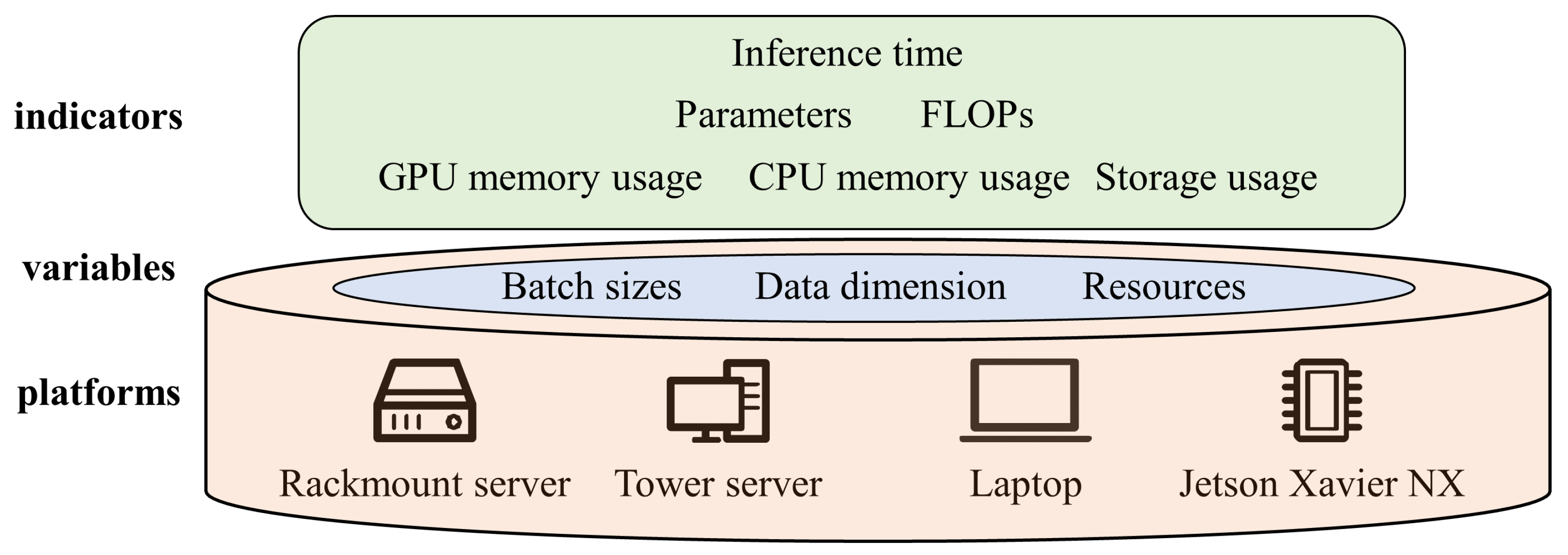
  • To assess model complexity, we developed a multi-dimensional evaluation system. This system includes a variety of metrics, including the number of parameters, floating point operations (FLOPs), storage usage, memory usage, and inference time, to provide a thorough and comprehensive evaluation of the model’s complexity.

2. Methods

2.1. Problem Formulation

Modulation classification can be treated as a multi-class decision problem. The goal of AMC methods based on deep learning techniques is to use a large amount of data to train and optimize a deep neural network model to identify the types of modulated signals. This involves two core elements: training data and a deep neural network model. The data mainly include data size, preprocessing, and distribution. The model is mainly concerned with the number of parameters, feature extraction ability, and inference efficiency. These directly determine the overall performance of the AMC methods. Figure 1 shows randomly selected examples of the IQ components and constellation diagrams for ten different modulation types from the 2016A dataset with SNR = 18 dB (It is worth noting that the modulation signals presented in the figure do not include AM-SSB modulation because our analyses reveal that the AM-SSB signals in the dataset do not match the characteristics of this type of signal and may only be channel responses. As a result, we removed this modulation-type data from the 2016A dataset.) However, there are differences between the IQ components or constellation diagrams. It is challenging even for a domain expert to distinguish between them owing to channel impairment. For example, QAM16 and QAM64 belong to the same modulation family, even with high SNRs, and it is difficult to visually distinguish them from the IQ components or constellation diagrams. As a result, we require models with strong feature extraction abilities that can also tackle the challenges presented by low data volumes, high signal noise, and high-order modulated signals.
The input of the deep neural network model is a complex base-band time-series representation of the signals received by the receiver. That is, we sample the IQ components of a radio signal at discrete time steps to obtain a 1 × N complex-valued vector y c . The real form of IQ samples on the receiver side is expressed as follows:
y r = [ ( y c ) T , ( y c ) T ] T = [ y ( 1 ) , y ( 2 ) , , y ( N ) ] T
Deep learning-based AMC methods can build an end-to-end pipeline. After feeding the radio signals into the model, the deep neural network will automatically extract the signal features and output category information.
Mean cross entropy is commonly used as a loss function in multiclass classification problems. The network training process can be transformed into an optimization problem, where f is the objective function. The goal of network training is to minimize f ( w ) for a dataset containing L samples in order to optimize the weight vector w of the network. The weights are iteratively updated such that w k w k + 1 using samples of batch size B k . Typically, SGD and its variants [20] are employed as optimizers.
min w n f ( w ) : = 1 L i = 1 L f i ( w )
w k + 1 = w k η 1 B k i = 1 B k f i ( w k )
where η denotes the learning rate.

2.2. Network Architecture

Although the computational speed has improved owing to the rapid development of hardware, deep learning tasks are still severely constrained by the memory and processing power of real-world applications. Therefore, to retain performance, we want the network model to be more lightweight. The SE-MSFN [5] is a representative and extremely malleable network framework. The SOTA performance has been attained on numerous open-source benchmark datasets. Although it builds fundamental modules using only convolution, it is faster and requires less memory than RNN-type models with complex parameters (such as MCLDNN [11] and LSTM2 [8]). SE-MSFN remains too large for edge devices in AMC tasks.
The lightweight design of the deep learning model is no longer limited to the design of tiny networks because of the extensive use of lightweight modeling techniques such as pruning [21], quantization [22], and knowledge distillation [23]. As a result, we believe that designing a high-accuracy network using lightweight thinking is more valuable than directly designing a tiny model. That is, the core principle of network design in this study is to maximize network performance while effectively reducing model complexity. As a result, we expect the proposed high-accuracy model to outperform current SOTA models, such as SE-MSFN [5], LSTM2 [8], and MCLDNN [11], among others, in terms of classification performance, while having a significantly smaller model size. Compared to existing lightweight models, for example, DAE [9] and LBNet [4], on various platforms, the proposed model can significantly reduce the inference time while maintaining high classification accuracy.
Figure 2 shows the overall structure of LENet-L and LENet-T, while scaling the above two models yields LENet-M and LENet-S. LENet-L is the most complex model in the LENet family, which is divided into three branches: IQ, amplitude and phases (APs), and EF. An input module, a head module, an automated feature extraction module, and a fusion module comprise the entire network. LENet-L is the only network that uses the APs branch. LENet-T and LENet-S do not use HOCs as additional feature branches to improve inference efficiency. LENet-M and LENet-S use a simpler SCCS with SE module than LENet-L, which uses MBConv. There is no skip-connection between the main LENet-T modules, which we believe is critical for improving efficiency of the model. Table 1 details the configuration information of each model in the LENet family.
Figure 3 depicts the core modules of the proposed LENet models. To achieve a trade-off between performance and computational cost, several hyperparameters in the model are set as follows: G = 2 for the channel shuffle (CS), r = 2 for the SE module, and n = 4 for the header block2.
Below is a brief description of each model in the LENet family.
LENet-T is a tiny model for edge devices with limited computational power. Because it does not use multi-scale patterns in its feature extraction backbone module, it uses only one skip connection in the header block to improve the model’s performance, ensuring that the model captures more discriminative features. We believe that the header block is critical and that the model should be configured based on the data characteristics and feature extraction backbone module. For example, if both the header block and feature extraction backbone are strong for data with a sample length of 128 and a few higher-order modulation types, such as 2016A, they could easily lead to overfitting the data. Consequently, we use a more complicated header block in LENet-T. The structure of Head block2 is shown in Figure 3. We start by feeding the original signals into a standard convolution of stride 2 and then building a skip connection with a pointwise convolution. The backbone consists of four SCCS (n = 4) modules and a DConv convolution.
LENet-S is positioned as a model with balanced performance and complexity, that is, an effective model that employs a simpler header block than LENet-T while employing a multi-scale feature extraction and fusion model in the feature extraction backbone, slightly increasing the complexity of the model but significantly improving the classification performance.
Both LENet-M and LENet-L are high-accuracy models. By scaling up the filter and convolution kernels and adding a domain knowledge-based feature extraction branch, LENet-M improves the feature extraction capability of the model. LENet-L adds a new input to LENet-M, resulting in a model with two feature extraction backbone branches, thereby increasing the model’s complexity and feature extraction diversity.
The following is a more detailed model design concept:
1. Lightweight modules are used to build the basic modules of the network. Existing high-accuracy models can effectively extract the spatial and temporal features of the original signals; however, such models typically have high model and computational complexities. The proposed LENet models employ DConv and SConv. Compared with standard convolution, DConv only performs convolution on each channel separately, and SConv first performs a DConv operation followed by a 1 × 1 pointwise convolution operation that mixes the resulting output channels. This factorization significantly reduces the computational cost and model size [14]. This study mainly uses depthwise separable convolution with a channel shuffle (SCCS) [16] to build the basic module. The SCCS module can provide an excellent balance between representation capability and computational cost.
The 1D convolutional layer is parameterized as follows:
C i , C o , f , k , s , h i , h o
where C i and C o represent the numbers of channels in the input and output feature maps, respectively. f is the number of convolutional filters with values equal to C o , k is the dimension of the 1D convolutional kernel, s is the convolution stride, and h i and h o are the input and output feature map dimensions, respectively. Ignoring the bias and assuming a stride of one and padding, the number of parameters for the standard convolution, DConv, and SConv are P s , P d c , and P s c , respectively.
P s = k × C i × f P d c = k × C i P s c = k × C i
The FLOPs metric is commonly used to measure the complexity of deep neural network models [9,14,15,16,17]. The FLOPs for standard convolution, DConv, and DSConv are F s , F d c , and F s c , respectively.
F s = 2 × k × C i × f × h i × h o F d c = 2 × k × C i × h i × h o F s c = 2 × k × C i × h i × h o + C i × f × h i × h o
It is clear from the above equations that using DConv and SConv instead of standard convolution can significantly reduce the number of parameters and FLOPs. However, neither of these two convolutional modules can alter the number of feature channels. Pointwise convolutions can help with information fusion between channels and change the dimensionality of channels. Even so, using pointwise convolutions in lightweight networks is not cost-effective. A CS operation can accomplish this in an efficient and elegant manner. Considering a convolutional layer with g groups whose output has g × n channels. In the SCCS module, we perform CS operation by first reshaping the output channel dimension into ( g , n ) , transposing it, and then flattening it back as the input of the next layer [16].
Additionally, since multiplexing greatly decreases model efficiency, we believe that residual connections and multi-branching structures should be present at the absolute minimum in lightweight models. As a result, LENet-T uses a simple serial structure.
2. Utilize the attention mechanism to boost the model’s capacity for feature extraction. We employ squeeze-and-excitation (SE) attention [17]. In order to learn the relationship between each channel and determine the weight of various channels, the SE mechanism first squeezes the feature map to acquire the global feature of the channel level. It next executes an excitation operation on the global feature. To obtain the final feature, the original feature map is multiplied. With the assistance of this attention mechanism, the model is able to suppress the unimportant channel aspects and focus more on the features of the channel that contain the most information. Another consideration is the SE module’s generic nature, which makes it simple to integrate into the network architecture. In our model, we use SE attention at almost every stage of the model, and although this will increase the number of parameters in the model, it will significantly improve the model’s ability to recognize signals with low SNRs.
3. Multi-scale feature extraction and fusion. Recent developments demonstrate that SOTA performance may be achieved over a wide range of deep learning tasks using multi-scale feature representation learning [5,24]. Due to this, as the number of network layers rises, the network’s receptive field gradually expands and its capacity for semantic representation rises as well. However, this also significantly reduces the signal’s resolution, resulting in the increasingly blurry appearance of many finely detailed features after multi-layer convolution operations. The retrieved features from the shallow neural network are less semantic but have a narrow receptive field and a good capacity to convey precise information. As a result, we use a cascaded multilevel network to extract the multi-scale features of the signals and a multi-scale feature fusion method to improve the model’s feature extraction capability to obtain powerful semantic features. Then, as illustrated in Figure 3, we develop two different types of convolution modules: MBConv with SE [14,15] and SCCS with SE in cascaded form, to extract robust and discriminative features from noisy radio signals. Since SCCS is lighter than MBConv, it is used in LENet-T, LENet-S, and LENet-M. Using HRNet [24] feature fusion mode, the feature output from two cascaded blocks is fused in the fusion and output stages. During the classification stage, global average pooling (GAP) is used to obtain the aggregated features. Using the SoftMax function, the output is further converted to the likelihood that the input signal belongs to each potential modulation type.
4. Improve the backbone network by adding more feature branches. The features of the signal, such as higher order statistics (HOS), higher order cumulants (HOCs), spectral correlation function, cyclic correntropy spectral density, etc., are often retrieved manually in classic feature-based AMC systems [25,26]. The features are then fed into the classifier, e.g., such as a decision tree, a support vector machine, or a multi-layer convolutional network, for testing and training; however, it can be problematic to get superior classification performance with these techniques. It is challenging to accurately capture the signals so that the classifier can achieve strong generalization ability since manual characteristics are biased.
As a result, we augment the deep neural network with the manually derived HOCs to improve the model’s classification performance. The HOCs [18] of the signals are extracted as an additional EF branch. In the feature extraction stage, we first reshape the data from N × 2 to N × 2 × 1 ; thus employing a 2D CNN. The first convolution layer adopts standard convolution, which can effectively preserve the spatial relationship between the IQ components because the I and Q components at each time step have strong correlations.
Furthermore, in LENet-L, we also build a branch in parallel with the backbone network using the APs of the signal converted by the IQ components to produce discriminative classification features. Finally, before GAP, the features extracted from the two branches are concatenated. The model would have to be twice as large as before as a result. At the same time, large-scale models run the risk of overfitting for small datasets.
5. By adjusting the network width, depth, and convolution kernel sizes and modules, the proposed model can be scaled for different resource constraints. We configure the LENet models with custom modules and parameters { f , k s , d }, resulting in a series of models, namely, LENet-T, LENet-S, LENet-M, and LENet-L, where f is the number of output filters in the convolution and k s is the size of the convolution kernel. The units of the dense layer in the additional EF branch are represented by d. Table 1 lists configuration information.
Equation (3) describes the mathematical representation of a deep neural network from an optimization point of view. Considering the inputs x and outputs y of the neural network, we can represent the proposed LENet as a deep neural network with M layers as the composition of M functions [27].
y = F ( x ; θ ) = ( f M f 1 ) ( x )
where ∘ denotes the composite mapping. Each f i is dependent on the parameter θ i , and θ represents the parameter set θ 1 , θ 2 , , θ M . Thus, for LENet-T, LENet-S, LENet-M, and LENet-L, contain different layers of the network, i.e., have different M. Thus, when a sample is input, the output will be different due to the difference in network structure.
Table 1 shows that only the raw IQ components of the signals are used as the model’s input in the lightweight model LENet-T. This is due to the shallow depth of LENet-T and the small number of feature maps, i.e., filters, f = 16. The feature’s dimension in the GAP layer is only 32. The fused features will be difficult to distinguish between primary and secondary if the HOCs branch is used, affecting the final decision output.
Additionally, LENet-T employs a more intricate residual structure in the head module. This is due to there being only one SCCS module with SE in LENet-T’s feature extraction module. Enhancing the feature extraction ability of the head module is therefore helpful for boosting the feature extraction ability, which greatly reduces computation cost while maintaining accuracy. Downsampling and upsampling are not included in the feature fusion step exactly because the feature extraction module of LENet-T has just one scale.

2.3. Incorporating Domain Knowledge to Create CNN-Based Models

Modulated signals have unique properties that distinguish them from image, audio, and textual data.
1. Intraclass diversity. As shown in Figure 4, The characteristics of the same class of signals in the time-frequency domain may differ significantly for different SNRs. Both the IQ component and the constellation diagram gradually drown in noise due to the influence of channel impairments such as center frequency offset, sample rate offset, additive white Gaussian noise, multipath, and fading. This makes it difficult to extract effective signal features for signal classification.
2. Inter-class similarity. Signals from different classes may demonstrate similar features in the time-frequency domain owing to the influence of channel impairments. As illustrated in Figure 1, several members of the same family of radio signals, such as QAM16 and QAM64, have strikingly similar properties in the time-frequency domain, even under high SNR conditions. In addition, this circumstance could arise among the various modulation families. For instance, at SNR = 10 dB, AM-DSB and WBFM in Figure 4 exhibit striking similarities in their properties. The IQ components of AM-DSB and WBFM are challenging to identify when the SNRs are low, such as SNR < 0 dB, as shown in Figure 4b,c, the IQ components of AM-DSB and WBFM are difficult to show their distinguishing characteristics. This leads to confusion between the classes.
3. Serial correlation. The modulated signal data takes the form of an N × 2 dimensional strip array with I and Q components, each of which has strong correlation and physical properties.
Considering the above characteristics of the modulated signals, three methods incorporating domain knowledge are used to build the CNN model: an additional expert feature extraction branch, a practical random data augmentation method, and a k × 2 convolution kernel. The additional feature branches allow the model to acquire more discriminative features. By focusing on the correlation between the I and Q components, the k × 2 convolution kernel improves the relevance of feature extraction. Data augmentation methods reduce the impact of noisy data by transforming the original data while improving the generalization ability of the model.
The HOCs are estimated from the received signal and are effective discriminators for many feature-based methods [2,18]. Generally, HOCs can be expressed as functions of high-order moments (HOMs). For a received signal y c , let M p q = E [ y c p q ( y c * ) q ] be the pth order moment, where q is the power of the complex conjugate signal y c * . The HOMs used for the EF branch in the proposed model include C 20 , C 21 , C 40 , C 41 , C 42 , C 60 , C 61 , C 62 , and C 63 . The relationship between the HOCs and HOMs is summarized in the literature [18]. Common relational expressions are given as follows.
C 20 = M 20 C 21 = M 21 C 40 = M 40 3 M 20 2 C 41 = M 40 3 M 20 M 21 C 42 = M 42 M 20 2 2 M 21 2 C 60 = M 60 15 M 20 M 40 30 M 20 3 C 61 = M 61 5 M 21 M 40 10 M 20 M 41 30 M 20 2 M 21 C 62 = M 62 6 M 20 M 42 8 M 21 M 41 M 22 M 40 + 6 M 20 2 M 22 + 24 M 21 2 M 20 C 63 = M 63 9 M 21 M 42 + 12 M 21 3 3 M 20 M 43 3 M 22 M 41 + 18 M 20 M 21 M 22
The proposed algorithm has a theoretical computation complexity of O ( M N ) [25]. N is the total length of the signal, and M is the order of the high-order transform.
The APs of modulated signals are generally used as the input of the RNN structure network [8,28], indicating that the APs contain rich signal features in comparison to the original IQ representation. As a result, we feed them into a feature extraction branch of LENet-L, and the conversion relationship between IQ and AP is as follows:
A = I 2 + Q 2 ϕ = arctan 2 ( Q / I )
The phase, which is expressed in radians, is normalized between −1 and 1, and the amplitude vector is L2-normalized.

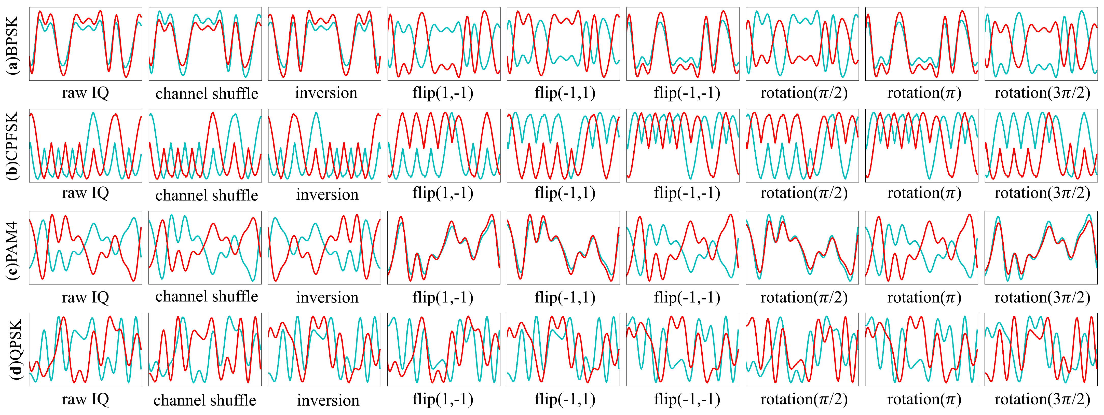
2.4. Random Data Augmentation for AMC

The model becomes sensitive to samples with low SNRs and forms memories for training data, decreasing the model’s ability to generalize on new datasets. Deep neural networks for AMC are powerful, but they exhibit undesired behaviors, particularly in the absence of a huge amount of data. It has been demonstrated that using data augmentation techniques for the APs of the modulated signals increases the accuracy of signal classification tasks [28]. However, data augmentation methods that excel on one dataset could struggle with another. Similar incidents may occur in various neural network models. Numerous automatic data augmentation techniques, such as AutoAugment [29], have been suggested as a result. However, such search algorithms are extremely sophisticated and require a large search space. The effectiveness of data augmentation is strongly influenced by the quantity of the target dataset and the deep neural network model. RandAugment [30], a random data augmentation strategy for vision problems, employs a straightforward grid search approach. It is constructed from augmentation transforms such as color jitters, rotation, and random crops. This method is straightforward and has low computational complexity. However, these transformations cannot be applied directly to radio signals.
SigAugment [31] is an automated data augmentation method specifically designed for modulated signals, and it has shown outstanding performance on small sample sizes and unbalanced category datasets.
The lightweight model proposed in this paper has a small capacity of only 4610 trainable parameters. SigAugment, as a regularization technique, is mainly used to suppress overfitting of the model, which may lead to underfitting if a very strong data augmentation strategy is used. Therefore, we selected only four transformations from the transformation pool: rotation, flip, channel shuffle, and inversion. Figure 5 illustrates these four transformations in detail.

2.5. Strategy for Hyperparameter Optimization

Along with network models, data quantity, and annotation quality, recent deep learning-based projects have also shown the impact of hyperparameters such as learning rate, batch size, and optimizer. There are contradictory results from existing studies on the effect of batch size on model classification effectiveness [32,33,34,35]. Research conducted on the MNIST and CIFAR-10 datasets has found that classification accuracy increases with batch size [32]. The majority of research contends that, particularly when the data set is small, lowering the learning rate and employing small batches can improve the model’s training. Large batch sizes can significantly speed up model training by improving the effectiveness of parallel computing [33,34,35], but small batch sizes can make the model converge more quickly and robustly than large batch sizes. These studies investigated the impact of batch size on convergence speed and accuracy in visual tasks from the perspective of gradient updates.
Batch sizes B k in existing studies are typically set to powers of two, such as 16, 32, 64, and 128. However, there is a significant distinction between communication and image data. DueB.wing to the presence of channel impairment, the SNR of the sample fluctuates over a wide range during the modulation signal classification task, for example, −20 dB to 30 dB. This leads to a significant difference between the samples with different SNRs belonging to the same modulation category. When training the neural network, we divide the out-of-order samples into batches and feed them into the network. The loss function of the tiny gradient representation network is slightly variable in each batch update parameter process when utilizing a small batch size, especially for modulation signal data with a wide SNR range, indicating that the gradient update is noisy. The network steadily updates the parameters along the direction of the loss function if a large batch size is utilized, especially for small datasets, which is not good for the model’s training. This implies that the acute minima can be eliminated more easily with small batch sizes. At the same time, it’s important to remember that the term “small” used here refers to the size of the training dataset as a whole. In other words, we cannot set the batch size too small because this will not only fail to improve performance but will also reduce training efficiency. Therefore, the strategy presented in this study enables flexible batch size selection, depending on the size of the dataset.

3. Results and Discussion

3.1. Experimental Settings

To verify the superiority of the proposed LENet models, we conducted quantitative modulation classification experiments on the 2016A, 2016B, and 2018A datasets. The 2016A and 2016B datasets are synthetic datasets generated with GNU radio, comprising 11 and 10 modulation types with 220,000 and 1,200,000 samples, respectively. It should be noted that because the AM-SSB modulation signals could only be the channel response, they are removed from the 2016A dataset. The dimension of each sample is 128 × 2. The 2018A dataset contains 24 modulation types, each of which is provided at 26 different SNR values ranging from −20 dB to 30 dB with 2 dB intervals, providing a total of 2,000,000 samples. Each sample has a length of 1024. Channel impairments primarily include the frequency offset, sample rate offset, and AWGN. To facilitate a fair comparison, we follow the strategy used in most studies and divide the 2016A and 2016B datasets into training, validation, and test sets at a ratio of 6:2:2 and the 2018A dataset at a ratio of 8:1:1. More details on the division of the data set can be found in Table 2. All the models are trained for 300 epochs using the Adam optimizer and categorical cross-entropy loss. All accuracy results, unless otherwise specified, are based on the test dataset.
In addition, our hyperparameter optimization strategy is as follows: we set different batch sizes for datasets of different sizes. For example, we train the 2016A, 2016B, and 2018A datasets with two graphics processing unit (GPU) cards and set the batch sizes to 128, 512, and 2048, respectively. We adopt a cosine schedule and a warm-up strategy to adjust the learning rate. The initial learning rate is set to 4 × 10 4 . The training process is terminated when the validation loss do not drop for 50 epochs or when the number of training epochs reaches 300. TensorFlow [36] is employed to train the models, and all the models are trained using two Tesla P100 or TITAN V GPU cards. Our hyperparameter optimization strategy improves the performance of the SOTA models used for comparison. We use the above hyperparameter optimization strategy to train SOTA models for comparison and discussion, and the settings for training SOTA models in the original literature are only used for the first set of comparison experiments for a fairer comparison. The deep learning framework utilized for all deep learning models is TensorFlow 2.5.0.
The 2016A dataset contains 20,000 samples of each modulation type and 1000 samples for each SNR. The results of training the model on such a small dataset are subject to large fluctuations. Consequently, all experiments on the 2016A dataset are repeated three times to improve experimental reliability. Owing to computational power constraints, data augmentation, ablation studies, and complexity analysis experiments are conducted using the 2016A dataset.

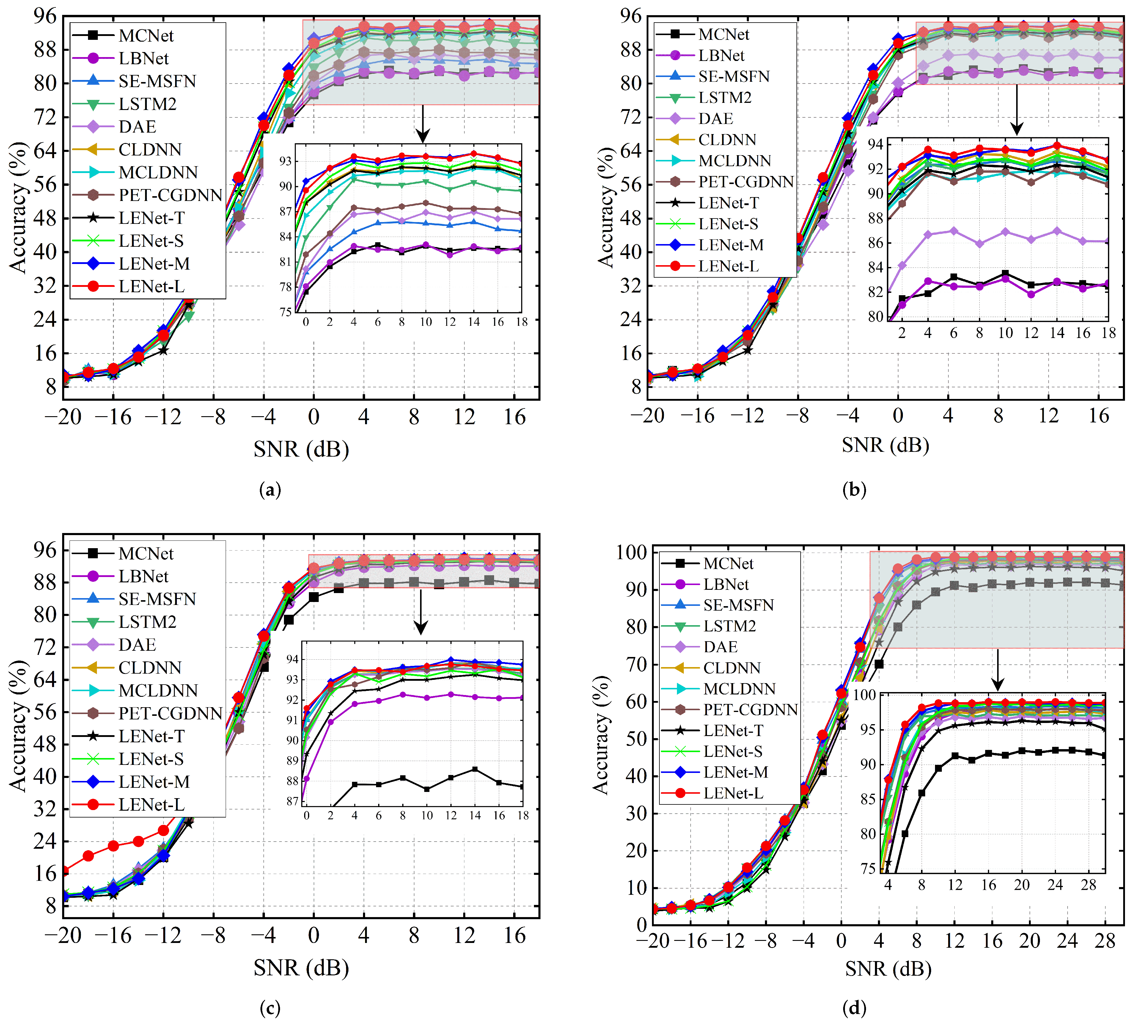
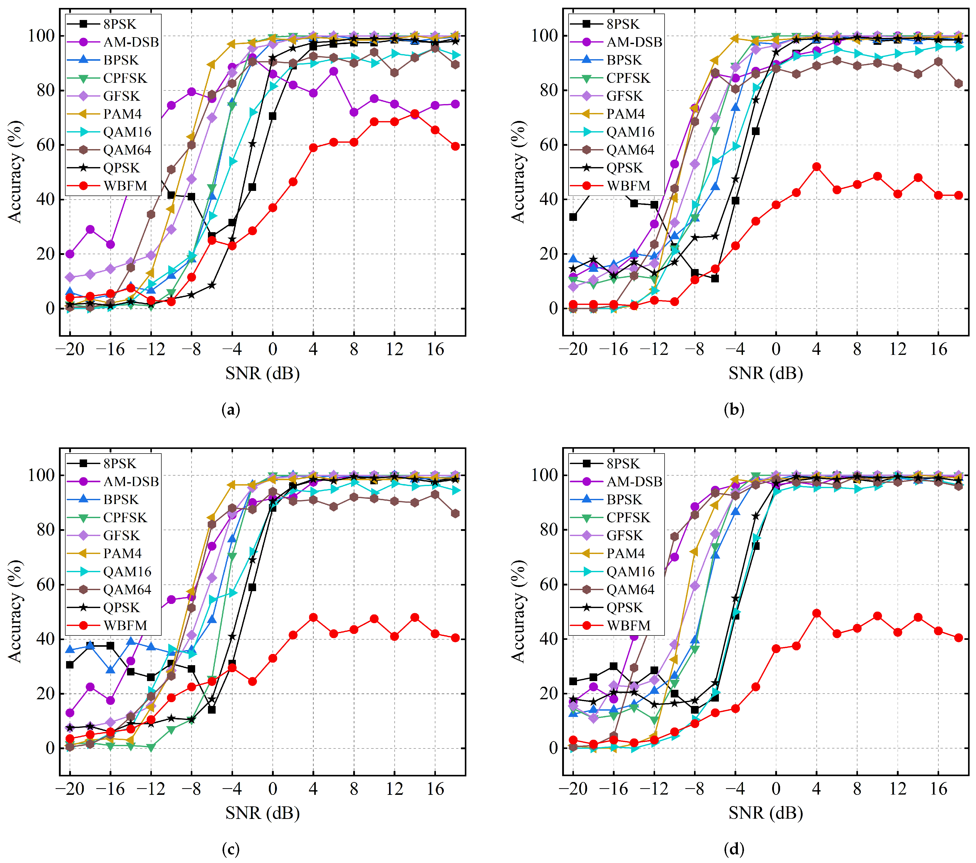
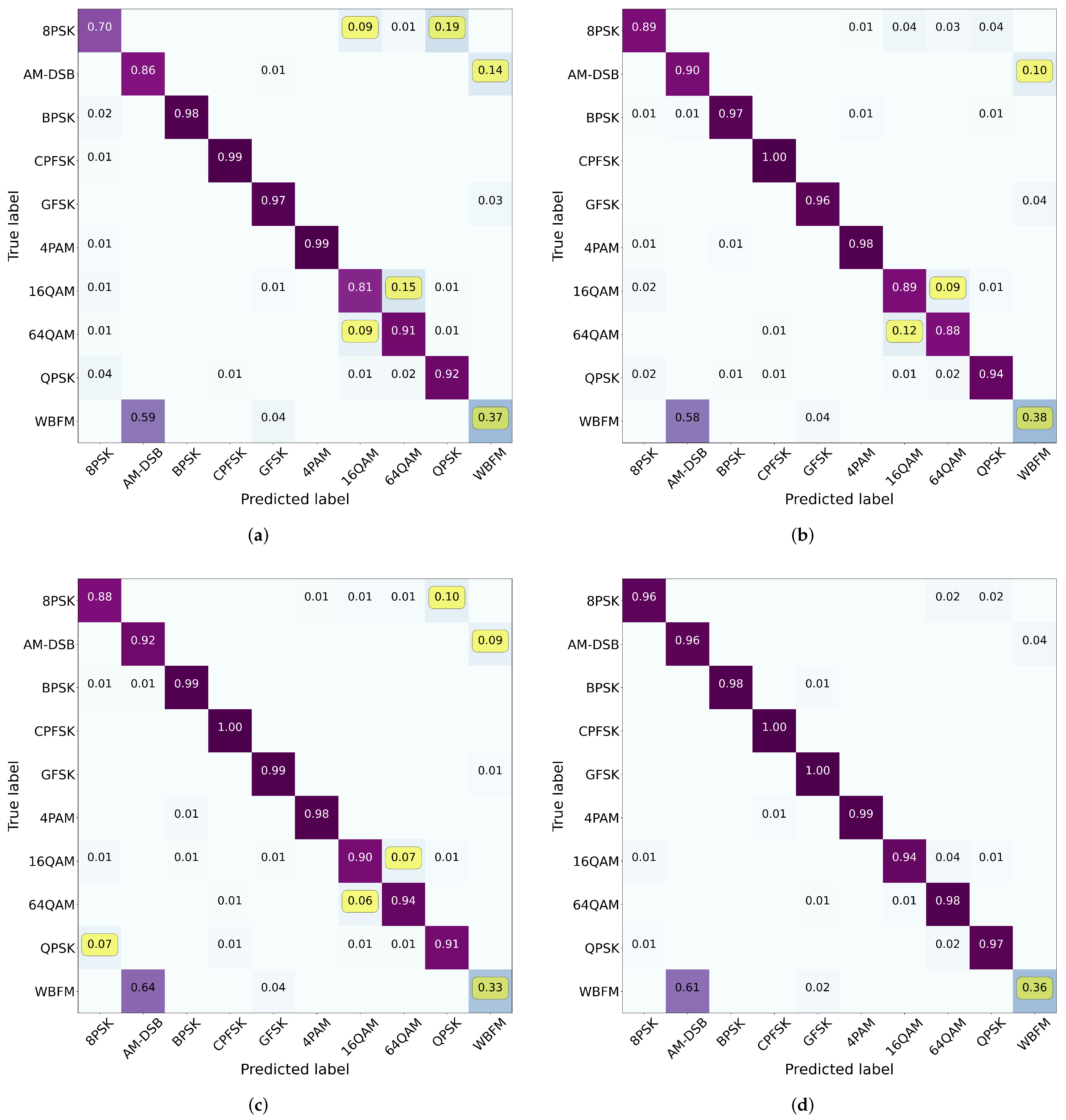
3.2. Comparison with SOTA Models

To evaluate and compare the model complexity and performance, several metrics are used, including the number of parameters, FLOPs, inference time, average classification accuracy, and highest classification accuracy. FLOPs is widely used to measure the complexity of deep neural network models. However, it is not a comprehensive measure of the complexity of a model. The final speed of a model is affected by factors such as memory bandwidth, optimization, central processing unit (CPU) pipeline, and cache, in addition to the amount of computation. As a result, we also provide a model’s inference time metric, which measures the model’s speed by running it 10 times in a row and taking the average elapsed time. This greatly reduces the error caused by processors or GPUs performing other tasks while the test is running.
The SOTA benchmark models used for comparison include lightweight models, including LBNet [4] and DAE [9], efficient models, including MCNet [3], and PET-CGDNN [12], and high-accuracy models, including SE-MSFN [5], LSTM2 [8], CLDNN [10], and MCLDNN [11]. In addition, when implementing the DAE, we removed the dropout layer after repeated tests because dropout in our experiments would make it difficult to match the results in the original literature by drastically reducing the performance of the DAE. When implementing the RNN structural models, for example, LSTM2 [8], CLDNN [10], and MCLDNN [11], and DAE [9], we use CuDNNLSTM instead of LSTM units for CUDA parallel processing to accelerate model training and inference.
Figure 6 shows the mean of the classification accuracy curves achieved by the 12 models over all SNRs on the three benchmark datasets. Because of the small size of the 2016A dataset, the results are obtained by taking the average of three experiments to increase the reliability. Figure 6a,b and Table 3 show that using our proposed hyperparameter strategy improves the performance of all SOTA models. Our proposed models, on the other hand, achieve better classification accuracy across all SNR intervals. They outperform the existing model by 3.04%, 0.69%, 0.62%, 1.41%, and 0.53%, respectively, in the five SNR intervals and the highest accuracy. It is worth noting that our lightweight model LENet-T outperforms the current SOTA lightweight models (e.g., LBNet, DAE). The SOTA average recognition accuracy over all SNRs achieved by our high-accuracy model LENet-M is 64.63% (the results of the three experiments are 64.72%, 64.43%, and 64.73%, respectively). The accuracy curves and statistical results of the existing models employing our hyperparameter optimization method are illustrated in Figure 6b and Table 3. The results show that our hyperparameter optimization strategy can greatly improve the performance of existing models.
Comparing Table 3, Table 4 and Table 5 reveal that our high-accuracy models LENet-M and LENet-L outperform existing SOTA models for almost all SNRs. The gains of our proposed models are most noticeable at low SNRs, e.g., in the 2016A dataset, where LENet-M outperforms SE-MSFN, LSTM2, CLDNN, and MCLDNN by 2.85%, 2.04%, 7.49%, and 2.39% on −10 dB to −2 dB, respectively. LENet-T outperforms LBNet and DAE in lightweight models by 3.21% and 3.92%, respectively. In particular, LENet-L outperforms the current best model SE-MSFN in the extremely low SNRs conditions from −20 dB to −12 dB, 7.17% higher, and 2.11% higher from −10 dB to −2 dB, with an average accuracy of 67.22% over all SNRs on the 2016B dataset. When the SNRs is higher than 8 dB on the 2018A dataset, the average accuracy of LENet-S, LENet-M, and LENet-L is 98.28%, 98.73%, and 98.86%, respectively. However, SE-MSFN, which has 98.17% classifcation accuracy, is the best model in the current model. Unfortunately, on the 2016 A dataset, LENet-L does not outperform LENet-M in classification performance. In contrast, LENet-L outperforms LENet-M on the 2016B and 2018A datasets, with the 2016B dataset being a larger version of the 2016A dataset. As LENet-L is trained on small-scale data, it may overfit the samples.
Subsequently, we chose the lightweight models DAE and LENet-T, as well as the high-accuracy models LSTM2 and LENet-M, as representative models to compare and analyze the recognition, confusion, and training convergence of each modulation type on the 2016A dataset. Figure 7 depicts the classification accuracy of representative models for various SNRs. The accuracy curves demonstrate that the following two aspects are indeed the common factors that affect the classification performance of the four models: On the one hand, even at high SNRs, it is extremely challenging to accurately identify WBFM signals. According to Figure 4c, the characteristics of the IQ components of the WBFM signals are elusive under different SNR conditions, and at 10 dB, the randomly selected samples show very similar characteristics to the AM-DSB signal. This seems to be primarily due to audio silence periods as modulated signals are generated from real audio streams [2]. On the other hand, as SNR falls below 0 dB, even for high-accuracy models, signal classification performance suffers significantly. It is worth noting that the proposed lightweight model LENet-T outperforms DAE at high SNRs for QAM16 and QAM64 signals.
Figure 8 illustrate the confusion matrixs for selected models at 0 dB on the 2016A dataset. Since the modulated signals are generated from real audio streams with silence periods, distinguishing AM-DSB and WBFM signals is difficult [8]. Due to the fact that QAM16 is a subset of QAM64, there is some confusion regarding the pair. Even so, we can clearly see that our proposed LENet-M outperforms LSTM2 in distinguishing between QAM16 and QAM64. Both LENet-T and LENet-M use data augmentation, SE modules, CS modules, and k s × 2 convolution kernels. The difference between the two models is that LENet-M has a larger model capacity, specifically a larger convolutional kernel, a deeper model structure, a larger number of filters and expert feature branches. The feature extraction capability of the model is therefore the main determinant of whether QAM16 and QAM64 can be effectively distinguished. Furthermore, the proposed LENet-T outperforms the DAE [9] in the recognition of 8BPSK, AM-DSB, QAM16, and QPSK signals.
Figure 9 shows the training process curves for the selected models. First, we notice that, in comparison to DAE, the validation loss and accuracy of LENet-T oscillate significantly in the early stage of training, and converge smoothly after 200 epochs while the convergence of training loss and accuracy is worse than that of DAE [9], and the validation loss and validation accuracy of LENet-T are better. The training and validation accuracy are nearly equal, indicating that the model avoids overfitting better and thus has better generalization performance. The training jitter may be caused by the fact that LENet-T has a small number of parameters and the model fluctuates in the validation set when using stronger data augmentation and simply takes longer to train to reach convergence. Convergence times for lightweight models are typically longer. Regarding the high-accuracy models, The LSTM2 is the fastest to converge, but the gap between training and validation accuracy is very big, the validation loss begins to rise after 30 to 40 epochs, and the model may overfit the training data. Our proposed LENet-M converges better and smoother than LSTM2 and outperforms it on the validation dataset.

3.3. Data Augmentation

The following two sets of experiments are conducted to study the impact of data augmentation on deep learning-based models. The first set of experiments evaluates the hyperparameter settings of SigAugment, and the results are listed in Table 6. The recognition accuracy of each SNR interval improved as the value of S increases. When S = 4, training LENet with SigAugment yields the best results on the 2016A dataset. As shown in the table, the model performance is more stable, the standard deviation of recognition accuracy is smaller for each SNR interval, and the full SNRs performance improvement is primarily due to signal classification in the [−10 dB, 2 dB] interval, whereas recognition performance at other SNRs does not differ significantly. This indicates that diversifying the data augmentation combinations used during the training phase substantially improves the model performance and increases the model’s robustness. As a result, the default value of parameter S is set to 4 in all subsequent experiments.
The second set of experiments verifies the effectiveness of the proposed random augmentation method when training LENet-S. The results are presented in Table 7. Compared to not using any data augmentation, the rotation, flip, channel shuffle, and inversion data augmentation methods alone improve the average accuracy of LENet-S on all SNRs by 1.22%, 0.39%, 0.70%, and 0.82%, respectively. The proposed method improves the average accuracy by 1.72%. The improvements in the [−10 dB, −2 dB], [0 dB, 10 dB], and [12 dB, 18 dB] intervals are 2.19%, 1.38%, and 1.22%, respectively. This indicates that the SigAugment method not only improves the model’s recognition performance for high SNR signals but also significantly improves the model’s recognition performance for low SNR signals.

3.4. Ablation Study

We also performed an ablation study to verify that each component of the proposed LENet models is critical. The experimental results are listed in Table 8. As can be seen, all components in LENet-M are indispensable in terms of performance improvement. The proposed data augmentation and SE attention mechanism have the greatest impact on LENet-M. Without these two components, the model’s average classification accuracy decreases by 1.45% and 2.21%, respectively. These reductions are primarily due to the very low SNRs intervals, e.g., −10 dB to −2 dB, which have accuracy reductions of 2.97% and 3.15%, respectively. The previous section discussed and analyzed the impact of the SigAugment approach in detail. In addition, our proposed model employs SE attention in multiple stages, making it well adapted to low-SNR signals. Furthermore, the EF branching and CS mechanisms slightly improve model classification performance. The incremental contributions of the average classification accuracy are 0.36% and 0.16%, respectively.

3.5. Complexity Analysis

We have created a framework to assess the complexity of deep learning models, with a focus on multi-platform compatibility. The framework diagram is shown in Figure 10. It consists of three main aspects: platforms, variables, and metrics. Platforms encompass servers, desktops, and edge devices, while variables refer to hardware and software resources, hyperparameters, input data size, etc., used throughout the model inference process. Model complexity is gauged through a combination of model-specific information and evaluation metrics gathered during testing.
We classified the comparison models into three categories: lightweight, effective, and high-accuracy. We evaluate the model’s complexity on various platforms in terms of the number of parameters, FLOPs, storage usage, memory usage, and inference time. The model import time, data preprocessing time, and result inference time are all included in the inference time. The results are the average of ten replicated experiments. Furthermore, since the CPU and GPU on the P4 platform share 8 GB of memory, we recorded the memory usage of the CPU and GPU on the P4 platform.
Four representative computational platforms are selected. Platform 1 is a Rackmount server powered by an Intel(R) 2.2 GHz Xeon(R) Silver 4114 processor and a Tesla P100 GPU card with a compute capability of 6.0. Platform 2 is a tower server that features a 3.10 GHz Intel(R) Xeon(R) Gold 6242R processor and a TITAN V GPU card with a compute capability of 7.0. Platform 3 is a laptop with a 2.3 GHz Intel(R) Core(TM) i7-11800H CPU and an Nvidia RTX3060 GPU card with an 8.6 compute capability. Platform 4 is the NVIDIA Jetson Xavier NX, an ultra small AI edge-end device for drones, portable devices, small robots, smart cameras, and high-resolution sensors. The device features a 6-core NVIDIA Carmel ARMv8 processor and a Xavier GPU with a computing capability of 7.2. Jetson Xavier NX uses a system-on-module architecture with 8 GB of memory shared between the CPUs and GPUs, and we choose the power mode: 20w, 6core. These platforms are denoted as P1, P2, P3, and P4, respectively.
As shown in Table 9, our proposed lightweight model LENet-T has the fewest number of parameters and inference time, where the number of parameters of LENet-T is 10.45% and 30.79% of those of LBNet and DAE, respectively. The inference times of LENet-T are 82.92%, 55.89%, 58.80%, and 86.31% of that of LBNet, and 77.23%, 46.16%, 40.38%, and 69.38% of that of DAE on the four platforms, respectively. Although DAE has the least FLOPs, its inference time is higher than that of LENet-T, due to the fact that CNNs do not have the sequence-dependence problem of LSTM, and thus can operate more efficiently in parallel. The gap between the model storage utilization and memory utilization of LENet-T and DAE is small. Except for edge-end platform P4, the memory utilization and inference time of the same model do not differ significantly across platforms. With an increase in GPU computing power, memory utilization generally increases and the inference time usually decreases.
The above inference time is obtained with a fixed batch size, whereas increasing the batch size typically increases memory consumption and improves the utilization of the GPU card, thus improving the processing efficiency, but only if the memory required for the processed data do not overflow. This highlights the importance of the memory usage of the GPU card, in addition to the inference time. In other words, a model with a small memory footprint enables the GPU to handle significantly more data concurrently, resulting in a faster processing time for equivalent batches of data. Additionally, when the batch size reaches a specific level, the larger the model, the more memory is consume. In particular, on the P4 platform, the GPU and CPU share 8 G of memory, and when the neural network performs inference on the GPU, the CPU must also process the task and occupy memory. The inference time results of the P4 platform are a concrete manifestation of this. For a single sample, our proposed lightweight model LENet-T requires approximately half the inference time of LBNet and DAE, whereas the average memory usage of LENet-T on multiple platforms is 43.02% and 111.56% for LBNet and DAE, respectively.
However, we also note that MCNet and CLDNN outperform LENet-T in terms of inference time when using a batch size of 128. In the following, we use four sets of experiments to gain further insight into the relationship between hardware platform, parameter settings and model inference time. We choose MCNet, LSTM2, CLDNN and LENet-T as representative as they illustrate the benefits of inference speed on different platforms. The experiments are: (1) the effect of batch size on inference speed on the server platform P2, (2) the effect of batch size on inference speed on the edge platform P4, (3) the use of CPU for inference, and (4) the effect of signal length on inference speed. The first three sets of experiments are performed on the 2016A test set, and the fourth set of experiments is performed on the 2018A dataset.
Table 10 and Table 11 show the inference speed and memory consumption of each model on the P2 and P4 platforms using different batch sizes. In general, the inference time decreases and then tends to be constant as the batch size increases. This may be related to the memory bandwidth of the device and the speed of data generation. On P2, LENet-T achieves the maximum gain in inference time at large batch sizes, followed by CLDNN and MCNet. On P4, increasing the batch size causes the LSMT2 and CLDNN models to quickly run out of memory, as the CPU and GPU in the device share 8 GB of memory. When the batch size is larger than 512, it is difficult to improve the inference speed of MCNet and LENet-T. Based on the above experimental results, we can see that: (1) an accurate representation of the inference speed of the models requires a comprehensive consideration of various factors such as batch size, device memory resources, model structure and model size; (2) models with small size, such as MCNet and LENet-T, usually occupy less memory. In this case, increasing the batch size appropriately according to the device situation can effectively improve the inference speed of the model. Such models are more advantageous on resource-constrained platforms.
The inference results on the CPU platform are shown in Table 12. Both LSTM2 and CLDNN use LSTM units to build their models, and these types of RNN-based networks are highly dependent on the underlying cuda acceleration for inference. To verify this, we used only CPUs for inference on the P4 platform. This scenario is common in real-world applications where many edge devices do not have embedded GPUs. The inference speed of MCNet is better than LENet-T because MCNet uses a smaller convolutional kernel than LENet-T, but LENet-T has a higher classification accuracy. As shown in Table 3, LENet-T outperformed MCNet with an average accuracy of 5.51% on the 2016A dataset. And in this paper, for all RNN networks, we used CuDNNLSTM instead of LSTM on the GPU platform to make a fair comparison.
Table 13 shows the model inference on the 2018A dataset. The signal length in 2018A is 1024. Compared to the signal length of 128, the FLOPs of LSTM2 increases from 1.32 M to 5.91 M, and the number of CLDNN parameters increases by a factor of 8. When the batch size is 128, these two models suffer from memory overflow on the P4 platform. However, MCNet and LENet-T have comparable time complexity.
In summary, LENet-T has a smaller size and consumes less memory on various platforms, and is therefore able to use a larger batch size, thus increasing inference speed. models with RNN structures, such as LSTM2 and CLDNN, require a greater sequence length of data and computational resources of the platform. LENet-M and LENet-L are recommended for applications requiring higher accuracy metrics, while LSTM2 and CLDNN are more suitable for resource constrained CPU or GPU edge computing platforms where a balance between accuracy and inference time is required.
In addition, it should be noted that the proposed high-accuracy model, LENet-M, has a significant time complexity overhead when using EF parallel branching, as the HOCs are computed using the CPU, while the GPU is parallelized only after data generation. This causes a dramatic decrease in GPU utilization, which is often only 2–3%. Additionally, the inference time of the model dramatically decreases when a more powerful CPU is used. Therefore, for scenarios with higher accuracy requirements in real-world applications, we advise employing larger-scale networks, such as LENet-M. Alternative optimization strategies include giving up the accuracy gain of the EF parallel branch focusing on achieving a tradeoff between speed and time complexity, or integrating the computation of HOCs onto GPUs to increase the effectiveness of the model’s parallel processing. Future work will study how our method can be applied to other scenarios, for example, testing data in real-world communication environments rather than data generated by GNU radio, few-shot learning, noise-oriented semi-supervised learning, higher-order modulated signal identification, etc. In particular, we wish to deploy our model on a mobile platform such as a UAV, and the algorithm can process the radio signals received from the receiver in real time.

4. Discussion

Q: “Data augmentation can significantly improve the performance of deep learning models, so is data augmentation enough for AMC tasks?”
From existing research, the gains from data augmentation for deep learning models are significant, especially when the data size is small and the categories are uneven. We can see this from recent work on this topic [28,31].
However, data augmentation does not solve all the problems in the AMC task. Data augmentation is a set of techniques to artificially increase the amount of data by generating new data points from existing data.The effect of increased data is to enhance the invariance of the model for certain transformations [37]. With regard to data augmentation methods, existing research has shown that the relative gain from applying data augmentation is smaller the more complex and the larger the data set. In other words, for complex and diverse data, the application of existing data augmentation approaches is still limited [38].
We conducted additional experiments on the 2016B dataset applying the same data augmentation strategy to train the LSTM2 model. Figure 11 shows a comparative analysis of LSTM2 and LENet-L, where the average accuracy of LSTM2 and LENet-L on 2016B is 65.25% and 67.22%, respectively. When the signal-to-noise ratio is high, the recognition accuracy of the two models is similar. However, when SNR <= −8 dB, LENet-L outperforms LSTM2 by 6.68%, 11.53%, 11.77%, 9.82%, 6.42%, 4.91%, and 2.68%. These findings highlight the need for further research to design superior models capable of addressing low signal-to-noise recognition challenges.
Additionally, regarding the 2016A dataset, the data augmentation methods significantly improve the performance of LBNet and MCNet models, but compared to other models of similar magnitude, these models still display a substantial accuracy gap, especially at low SNR. Consequently, the feature extraction model, acting as the primary body for feature extraction, plays a crucial role in enhancing performance, highlighting the need to identify superior feature extraction models.
Q: “How should we choose a deep learning model during engineering deployment and application?”
This is an open-ended question, and various factors must be considered to make an informed decision. Firstly, the application scenario must be carefully evaluated, as different scenarios have different performance requirements. For example, in contexts involving the offline analysis of massive signal datasets, signal recognition accuracy is more important than real-time responsiveness, necessitating the selection of a model with higher accuracy. On the other hand, in edge-based real-time recognition scenarios, where computing resources are limited, a more lightweight model should be chosen to meet the real-time requirements without compromising accuracy thresholds. Secondly, it is necessary to assess the performance of the device on which the model is running, as deep learning models require computational power for optimal performance. As such, the chosen model must be adaptable to the computing platform to ensure optimal performance.
Therefore, the CNN-based model family proposed in this paper presents a greater range of alternative options in the engineering deployment process, providing more avenues for selecting an appropriate model to satisfy the specific requirements of a given application scenario.
Q: “Is it better to have more transformations in the SigAugment transformation pool?”
Data augmentation, such as SigAugment, is frequently utilized to prevent overfitting in deep learning models, particularly in small sample conditions. However, the optimal number of transformations to include in the augmented transformation pool remains unclear.
The experimental results in Table 14 are used to investigate the relationship between the number of transformations in the transformation pool and the model. The results show that (1) data augmentation improves the performance of both LENet-T and LENet-M; (2) increasing the number of transforms does not consistently improve performance for the lightweight model LENet-T, but the accuracy of the model improves as the number of transforms increases for the more complex model LENet-M.
In addition, we added commonly used time-series data augmentations, including magnitude warping, time warping, window warping, and window slicing transforms [39], to SigAugment’s transform pool. While these transformations exhibited strong data fitness, our results demonstrate that their domain specificity adversely impacted model performance in the AMC task.
Therefore, boosting the performance of the model does not necessarily rely on an increase in the number of transforms included in the transform pool. Rather, the individual transforms need to be rigorously validated against the model and data to ensure that they are appropriate for the AMC tasks.
Q: “Existing approaches explore the AMC task in terms of data, models, hyperparameters, etc. What can be done in the future to extend this research?”
This paper explores deep learning models that can be used on different platforms from the perspective of AMC application deployment. Combined with the existing work, future work could be carried out in the following areas: firstly, making full use of the large amount of unlabeled data, combined with data augmentation methods, to carry out research in semi-supervised learning; secondly, moving out of the laboratory and validating existing models in real-world environments; and thirdly, investigating lower consumption models to adapt to platforms with extreme memory and computational resource constraints.

5. Conclusions

In this paper, we propose a family of AMC models based on domain knowledge for multi-platform deployment, validate their performance on typical servers, laptop, and edge computing device, and demonstrate the effectiveness of the proposed algorithm through the lightweight model’s inference speed advantage and the new SOTA performance achieved by the high-accuracy model on multiple benchmark datasets. Specifically, we have proposed a family of CNN-based networks for different platforms, namely LENet. LENet models were extensively tested on three benchmark datasets, and the results showed that the proposed algorithm achieved SOTA average classification accuracies of 64.63%, 67.22%, and 65.03% on the test set, which are 1.67%, 2.35%, and 0.57% higher than the existing SOTA model SE-MSFN. Notably, the main benefit of our model over existing models stems primarily from its effectiveness on signals with low SNRs. However, at the same time, our models have achieved SOTA top accuracies across SNRs, with 93.93%, 93.99%, and 99.03% on the three benchmark datasets, respectively. Furthermore, we propose a multidimensional and credible model complexity assessment framework that integrates platform, variables, and multiple assessment metrics to provide a more complete picture of the complexity of deep learning models. A comprehensive analysis of the complexity of the proposed algorithm using this framework has verified that LENet outperforms the RNN-based model in terms of complexity, especially when the dimensionality of the signals is large, and that LENet has a significant advantage in terms of memory resource consumption. Furthermore, the inference speed of the CNN-based network structure on a CPU platform has been shown to be significantly better than that of the RNN-based model. Moreover, we propose a set of hyperparameter optimization methods for datasets of various sizes, providing a fair comparison of hyperparameter setting schemes for future research. However, an open question remains as to how our algorithm further improves the recognition performance of signals with low SNRs. Taking the test results of LENet-L on the 2016B dataset as an example, although the recognition performance of LENet-L below 0 dB is significantly improved compared with the existing algorithm, there may still be a certain gap from practical deployment and application. Finally, we use HOCs parallel branch to improve the model’s performance, which is experimentally verified to be effective but also introduces a large amount of time overhead, so the selection of HOCs and how to better integrate them into the network remains an open question. Future work could focus on semi-supervised learning, realistic environment-oriented AMC models, and the construction of lower-power models.

Author Contributions

Conceptualization, S.W. and Z.W.; methodology, S.W.; software, S.W.; validation, S.W. and Z.W.; formal analysis, L.Z.; investigation, Z.L.; resources, Z.W.; data curation, S.W.; writing—original draft preparation, S.W.; writing—review and editing, H.M., S.W. and Z.S.; visualization, F.L., Z.L. and L.Z.; supervision, F.L., H.M. and Z.S.; project administration, H.M. and Z.S. All authors have read and agreed to the published version of the manuscript.

Funding

This work was supported in part by National Key R&D Program of China Grant No. 2022ZD0115300 and the Scientific Research Plan of the National University of Defense Technology under Grant No. ZK20-38 and YJKT-RC-2108.

Institutional Review Board Statement

Not applicable.

Informed Consent Statement

Not applicable.

Data Availability Statement

Data are available on request.

Conflicts of Interest

The authors declare no conflict of interest.

References

  1. Jagannath, A.; Jagannath, J.; Melodia, T. Redefining Wireless Communication for 6G: Signal Processing Meets Deep Learning with Deep Unfolding. IEEE Trans. Artif. Intell. 2021, 2, 528–536. [Google Scholar] [CrossRef]
  2. O’Shea, T.J.; Roy, T.; Clancy, T.C. Over-the-Air Deep Learning Based Radio Signal Classification. IEEE J. Sel. Top. Signal Process. 2018, 12, 168–179. [Google Scholar] [CrossRef] [Green Version]
  3. Huynh-The, T.; Hua, C.H.; Pham, Q.V.; Kim, D.S. MCNet: An Efficient CNN Architecture for Robust Automatic Modulation Classification. IEEE Commun. Lett. 2020, 24, 811–815. [Google Scholar] [CrossRef]
  4. Shi, F.; Yue, C.; Han, C. A lightweight and efficient neural network for modulation recognition. Digit. Signal Process. Rev. J. 2022, 123, 103444. [Google Scholar] [CrossRef]
  5. Wu, X.; Wei, S.; Zhou, Y. Deep Multi-Scale Representation Learning with Attention for Automatic Modulation Classification. In Proceedings of the International Joint Conference on Neural Networks (IJCNN), Padua, Italy, 18–23 July 2022. [Google Scholar]
  6. Meng, F.; Chen, P.; Wu, L.; Wang, X. Automatic modulation classification: A deep learning enabled approach. IEEE Trans. Veh. Technol. 2018, 67, 10760–10772. [Google Scholar] [CrossRef]
  7. Xu, Y.; Li, D.; Wang, Z.; Guo, Q.; Xiang, W. A deep learning method based on convolutional neural network for automatic modulation classification of wireless signals. Wirel. Netw. 2019, 25, 3735–3746. [Google Scholar] [CrossRef]
  8. Rajendran, S.; Meert, W.; Giustiniano, D.; Lenders, V.; Pollin, S. Deep Learning Models for Wireless Signal Classification with Distributed Low-Cost Spectrum Sensors. IEEE Trans. Cogn. Commun. Netw. 2018, 4, 433–445. [Google Scholar] [CrossRef] [Green Version]
  9. Ke, Z.; Vikalo, H. Real-Time Radio Technology and Modulation Classification via an LSTM Auto-Encoder. IEEE Trans. Wirel. Commun. 2022, 21, 370–382. [Google Scholar] [CrossRef]
  10. West, N.E.; O’Shea, T. Deep architectures for modulation recognition. In Proceedings of the 2017 IEEE International Symposium on Dynamic Spectrum Access Networks (DySPAN), Baltimore, MD, USA, 6–9 March 2017; pp. 1–6. [Google Scholar] [CrossRef] [Green Version]
  11. Xu, J.; Luo, C.; Parr, G.; Luo, Y. A Spatiotemporal Multi-Channel Learning Framework for Automatic Modulation Recognition. IEEE Wirel. Commun. Lett. 2020, 9, 1629–1632. [Google Scholar] [CrossRef]
  12. Zhang, F.; Luo, C.; Xu, J.; Luo, Y. An Efficient Deep Learning Model for Automatic Modulation Recognition Based on Parameter Estimation and Transformation. IEEE Commun. Lett. 2021, 25, 3287–3290. [Google Scholar] [CrossRef]
  13. Ge, Z.; Liu, S.; Wang, F.; Li, Z.; Sun, J. Yolox: Exceeding yolo series in 2021. arXiv 2021, arXiv:2107.08430. [Google Scholar]
  14. Sandler, M.; Howard, A.; Zhu, M.; Zhmoginov, A.; Chen, L.C. MobileNetV2: Inverted Residuals and Linear Bottlenecks. In Proceedings of the 2018 IEEE/CVF Conference on Computer Vision and Pattern Recognition, Salt Lake City, UT, USA, 18–23 June 2018; pp. 4510–4520. [Google Scholar] [CrossRef] [Green Version]
  15. Tan, M.; Le, Q.V. EfficientNet: Rethinking model scaling for convolutional neural networks. In Proceedings of the 36th International Conference on Machine Learning, ICML 2019, Long Beach, CA, USA, 9–15 June 2019; pp. 10691–10700. [Google Scholar]
  16. Zhang, X.; Zhou, X.; Lin, M.; Sun, J. ShuffleNet: An Extremely Efficient Convolutional Neural Network for Mobile Devices. In Proceedings of the 2018 IEEE/CVF Conference on Computer Vision and Pattern Recognition (CVPR), Salt Lake City, UT, USA, 18–23 June 2018; pp. 6848–6856. [Google Scholar]
  17. Hu, J.; Shen, L.; Albanie, S.; Sun, G.; Wu, E. Squeeze-and-Excitation Networks. IEEE Trans. Pattern Anal. Mach. Intell. 2020, 42, 2011–2023. [Google Scholar] [CrossRef] [PubMed] [Green Version]
  18. Abdelmutalab, A.; Assaleh, K.; El-Tarhuni, M. Automatic modulation classification based on high order cumulants and hierarchical polynomial classifiers. Phys. Commun. 2016, 21, 10–18. [Google Scholar] [CrossRef]
  19. O’Shea, T.J.; West, N. Radio Machine Learning Dataset Generation with GNU Radio. In Proceedings of the GNU Radio Conference, Boulder, CO, USA, 12–16 September 2016. [Google Scholar]
  20. Kingma, D.P.; Ba, J. Adam: A method for stochastic optimization. arXiv 2014, arXiv:1412.6980. [Google Scholar]
  21. Wang, Y.; Yang, J.; Liu, M.; Gui, G. LightAMC: Lightweight automatic modulation classification via deep learning and compressive sensing. IEEE Trans. Veh. Technol. 2020, 69, 3491–3495. [Google Scholar] [CrossRef]
  22. Zhang, Y.; Cui, M.; Shen, L.; Zeng, Z. Memristive quantized neural networks: A novel approach to accelerate deep learning on-chip. IEEE Trans. Cybern. 2019, 51, 1875–1887. [Google Scholar] [CrossRef]
  23. Ma, H.; Xu, G.; Meng, H.; Wang, M.; Yang, S.; Wu, R.; Wang, W. Cross model deep learning scheme for automatic modulation classification. IEEE Access 2020, 8, 78923–78931. [Google Scholar] [CrossRef]
  24. Wang, J.; Sun, K.; Cheng, T.; Jiang, B.; Deng, C.; Zhao, Y.; Liu, D.; Mu, Y.; Tan, M.; Wang, X.; et al. Deep High-Resolution Representation Learning for Visual Recognition. IEEE Trans. Pattern Anal. Mach. Intell. 2021, 43, 3349–3364. [Google Scholar] [CrossRef] [PubMed] [Green Version]
  25. Liu, X.; Li, C.J.; Jin, C.T.; Leong, P.H.W. Wireless Signal Representation Techniques for Automatic Modulation Classification. IEEE Access 2022, 10, 84166–84187. [Google Scholar] [CrossRef]
  26. Majhi, S.; Gupta, R.; Xiang, W.; Glisic, S. Hierarchical Hypothesis and Feature-Based Blind Modulation Classification for Linearly Modulated Signals. IEEE Trans. Veh. Technol. 2017, 66, 11057–11069. [Google Scholar] [CrossRef] [Green Version]
  27. Caterini, A.L.; Chang, D.E. Deep Neural Networks in a Mathematical Framework; Springer: Berlin/Heidelberg, Germany, 2018. [Google Scholar]
  28. Huang, L.; Pan, W.; Zhang, Y.; Qian, L.; Gao, N.; Wu, Y. Data Augmentation for Deep Learning-Based Radio Modulation Classification. IEEE Access 2020, 8, 1498–1506. [Google Scholar] [CrossRef]
  29. Cubuk, E.D.; Zoph, B.; Mané, D.; Vasudevan, V.; Le, Q.V. AutoAugment: Learning Augmentation Strategies From Data. In Proceedings of the 2019 IEEE/CVF Conference on Computer Vision and Pattern Recognition (CVPR), Long Beach, CA, USA, 15–20 June 2019; pp. 113–123. [Google Scholar] [CrossRef]
  30. Cubuk, E.D.; Zoph, B.; Shlens, J.; Le, Q.V. Randaugment: Practical automated data augmentation with a reduced search space. In Proceedings of the IEEE/CVF Conference on Computer Vision and Pattern Recognition (CVPR) Workshops, Seattle, WA, USA, 14–19 June 2020; pp. 3008–3017. [Google Scholar]
  31. Wei, S.; Sun, Z.; Wang, Z.; Liao, F.; Li, Z.; Mi, H. An Efficient Data Augmentation Method for Automatic Modulation Recognition from Low-Data Imbalanced-Class Regime. Appl. Sci. 2023, 13, 3177. [Google Scholar] [CrossRef]
  32. Radiuk, P.M. Impact of training set batch size on the performance of convolutional neural networks for diverse datasets. Inf. Technol. Manag. Sci. 2017, 20, 20–24. [Google Scholar] [CrossRef]
  33. Keskar, N.S.; Mudigere, D.; Nocedal, J.; Smelyanskiy, M.; Tang, P.T.P. On large-batch training for deep learning: Generalization gap and sharp minima. arXiv 2016, arXiv:1609.04836. [Google Scholar]
  34. Kandel, I.; Castelli, M. The effect of batch size on the generalizability of the convolutional neural networks on a histopathology dataset. ICT Express 2020, 6, 312–315. [Google Scholar] [CrossRef]
  35. Masters, D.; Luschi, C. Revisiting small batch training for deep neural networks. arXiv 2018, arXiv:1804.07612. [Google Scholar]
  36. Abadi, M.; Barham, P.; Chen, J.; Chen, Z.; Davis, A.; Dean, J.; Devin, M.; Ghemawat, S.; Irving, G.; Isard, M.; et al. TensorFlow: A system for Large-Scale machine learning. In Proceedings of the 12th USENIX Symposium on Operating Systems Design and Implementation (OSDI 16), Savannah, GA, USA, 2–4 November 2016; pp. 265–283. [Google Scholar]
  37. Zhang, H.; Cisse, M.; Dauphin, Y.; Lopez-Paz, D. mixup: Beyond empirical risk management. In Proceedings of the 6th Int. Conf. Learning Representations (ICLR), Vancouver, BC, Canada, 30 April–3 May 2018; pp. 1–13. [Google Scholar]
  38. Lewy, D.; Mańdziuk, J. An overview of mixing augmentation methods and augmentation strategies. Artif. Intell. Rev. 2023, 56, 2111–2169. [Google Scholar] [CrossRef]
  39. Iwana, B.K.; Uchida, S. An empirical survey of data augmentation for time series classification with neural networks. PLoS ONE 2021, 16, e0254841. [Google Scholar] [CrossRef]
Figure 1. (a) IQ components and (b) constellation diagram examples of 10 different modulation types from 2016A with SNR = 18 dB. The cyan line represents the in-phase component, whereas the red line represents the quadrature component.
Electronics 12 01820 g001
Figure 2. Overall structure of proposed (a) LENet-L and (b) LENet-T.
Electronics 12 01820 g002
Figure 3. Core modules of proposed LENet models: (a) SCCS module, (b) SE module, (c) Head block1, (d) Head block2, (e) MBConv module, and (f) fusion module.
Electronics 12 01820 g003
Figure 4. IQ components examples of (a) AM-DSB and (b) WBFM, constellation diagram examples of (c) PAM4 and (d) BPSK with SNR = −20 dB, −10 dB, 0 dB, 10 dB, and 18 dB. The cyan line shows the in-phase component while the red line shows the quadrature component.
Electronics 12 01820 g004
Figure 5. (a) BPSK, (b) CPFSK, (c) PAM4, and (d) QPSK samples from 2016A with SNR = 18 dB and various data augmentation methods. Where flip( α , β ) represents the flip of the IQ components. That is, −1 means switching the I or Q component value to its opposite, and 1 means remaining unchanged. The cyan line shows the in-phase component while the red line shows the quadrature component.
Electronics 12 01820 g005
Figure 6. Classification accuracy of all models against SNR on the (a) 2016A, (b) 2016A (hyperparameter optimization), (c) 2016B, and (d) 2018A dataset.
Electronics 12 01820 g006
Figure 7. Classification accuracy at each SNR and modulation type of (a) DAE, (b) LENet-T, (c) LSTM2, and (d) LENet-M on the 2016A dataset.
Electronics 12 01820 g007
Figure 8. Confusion matrix for (a) DAE, (b) LENet-T, (c) LSTM2, and (d) LENet-M at 0 dB on the 2016A dataset. Values less than 0.01 are not included. In the confusion matrix, values above 0.5 are indicated in purple; the darker the value, the greater the confusion. The higher the ambiguity, the darker the value. Yellow represents values between 0.05 and 0.5.
Electronics 12 01820 g008
Figure 9. (a) Training loss, (b) Training accuracy, (c) Validation loss, and (d) Validation accuracy curves of DAE, LSTM2, LENet-T, and LENet-M on the 2016A dataset.
Electronics 12 01820 g009
Figure 10. The framework for evaluating the complexity of deep learning models.
Electronics 12 01820 g010
Figure 11. Comparison of LSTM2 and LENet-L on the 2016B dataset.
Electronics 12 01820 g011
Table 1. Configuration information for LENet models.
Modules/ParametersLENet-TLENet-SLENet-MLENet-L
InputIQIQ + HOCsIQ + HOCsIQ + AP + HOCs
HeadHead block1Head block2Head block2Head block2
Feature extraction(SCCS + SE)*1(SCCS + SE)*4(SCCS + SE)*4(MBConv + SE)*4
FusionSCCS + SE + ActFusion blockFusion blockFusion block
f16163232
ks(8, 2)(8, 2)(15, 2)(15, 2)
d003636
Table 2. Details of the dataset division.
DatasetDataset SizeTraining SetValidation SetTesting Set
2016A200,000120,00040,00040,000
2016B1,200,000720,000240,000240,000
2018A2,555,9042,044,722255,591255,591
Table 3. Results of statistical analysis of all models’ classification accuracy on the 2016A dataset. The top2 for each statistic are highlighted.
StatisticsMCNetLBNetSE-
MSFN
LSTM2DAECLDNNMCL
DNN
PET-
CGDNN
LENet
TSML
−20∼−12 dB13.8813.7414.0413.6414.0213.4213.3213.6112.5014.0314.1713.96
−10∼−2 dB49.3950.4854.2051.3448.5052.3753.2551.4854.2456.7757.5656.51
0∼10 dB81.7481.6691.5091.3585.1491.9390.5690.3991.0692.2293.1992.63
12∼18 dB82.6482.4392.2692.2586.3992.7791.5691.2891.9192.8893.6993.36
−20∼18 dB56.8757.0462.9662.1058.4562.5862.1261.6562.3863.9464.6364.08
Highest accuary83.5383.0892.7292.8586.9893.4091.8792.0092.3393.7593.9393.93
Table 4. Results of statistical analysis of all models’ classification accuracy on the 2016B dataset. The top2 for each statistic are highlighted.
StatisticsMCNetLBNetSE-
MSFN
LSTM2DAECLDNNMCL
DNN
PET-
CGDNN
LENet
TSML
−20∼−12 dB13.5114.3514.9813.9014.6013.7513.7614.4713.2214.5413.8822.15
−10∼−2 dB53.5156.2058.0757.0356.0057.9657.8355.0155.7957.0459.5960.18
0∼10 dB87.0791.2092.8992.7592.6492.9993.0092.6891.9592.5593.0993.07
12∼18 dB88.1092.1693.6993.4893.4293.6993.6693.6193.1293.3593.8793.61
−20∼18 dB60.5063.4364.8764.2564.1264.5664.5363.9063.4664.3365.0767.22
Highest accuary88.5992.2893.8293.5693.5493.8093.8193.8793.2593.5293.9993.76
Table 5. Results of statistical analysis of all models’ classification accuracy on the 2018A dataset. The top2 for each statistic are highlighted.
StatisticsMCNetLBNetSE-
MSFN
LSTM2DAECLDNNMCL
DNN
PET-
CGDNN
LENet
TSML
−20∼−8 dB8.059.559.689.698.959.268.329.176.967.399.499.74
−6∼6 dB52.1557.7061.4661.5756.0556.5858.4158.2954.7558.4362.4662.34
8∼20 dB90.3397.0898.0697.1196.3697.2497.5997.4995.3298.0698.6698.81
22∼30 dB91.8197.8998.3397.0896.7297.5197.8797.9295.8998.5898.8398.93
−20∼30 dB58.1863.0764.4664.0062.0462.6663.0663.2460.7263.0864.9465.03
Highest accuary92.0898.0998.4597.3096.9797.8998.1298.1096.3398.7999.0299.03
Table 6. Accuracy of LENet-S with varying augmentation transformation parameters (S). The top1 accuracy for each SNR interval is highlighted.
S−20 dB∼−12 dB−10 dB∼−2 dB0 dB∼10 dB12 dB∼18 dBAll SNRsHighest Accuary
MeanStdMeanStdMeanStdMeanStdMeanStdMeanStd
013.880.6153.830.9590.090.9791.330.7462.220.3091.950.69
113.560.4755.930.6292.000.4192.940.4063.560.4093.700.39
213.690.3456.240.9392.210.2992.920.4563.730.4893.450.36
313.560.4755.930.6292.000.4192.940.4063.560.4091.950.69
414.030.2156.770.5892.220.3892.880.0963.940.2693.700.39
Table 7. Accuracy of LENet-S with varying augmentation methods. The top1 accuracy for each SNR interval is highlighted. w/o denotes without.
Methods−20 dB∼−12 dB−10 dB∼−2 dB0 dB∼10 dB12 dB∼18 dBAll SNRsHighest Accuary
MeanStdMeanStdMeanStdMeanStdMeanStdMeanStd
w/o augmentation13.880.6153.830.9590.090.9791.330.7462.220.3091.950.69
Rotation13.210.3055.880.1792.010.3092.800.3063.440.2093.450.25
Flip13.540.7853.610.9091.330.7392.150.6762.610.4892.880.59
Channel shuffle14.190.2654.360.5791.210.4692.110.6062.920.4692.820.38
Inversion14.590.5554.110.4691.350.6092.310.2863.040.4593.000.31
SigAugment14.030.2156.770.5892.220.3892.880.0963.940.2693.700.39
Table 8. Ablation study of different modules in LENet-M on the 2016A dataset. EF stands for expert feature branch. CS is the channel shuffle module. SE is the squeeze-and-excitation attention mechanism. 2D CK is the k s × 2 two-dimensional convolution kernel.
Methods−20 dB∼−12 dB−10 dB∼−2 dB0 dB∼10 dB12 dB∼18 dBAll SNRsHighest Accuary
MeanStdMeanStdMeanStdMeanStdMeanStdMeanStd
w/o augmentation14.720.8954.270.7590.900.2192.030.1062.930.2092.780.19
w/o EF13.490.4657.050.8992.430.2693.260.3264.020.4593.870.18
w/o CS13.960.3056.871.0992.690.3093.520.2064.220.3294.070.18
w/o SE13.110.4754.091.6990.411.5891.231.4162.171.1891.921.40
w/o 2D CK12.140.4056.480.6992.360.4492.840.2663.430.3093.530.28
Our model14.400.6557.240.8892.630.3793.390.2164.630.3293.930.25
Table 9. Complexity of different models on the 2016A dataset. Params is trainable parameters of the model. Size is the amount of storage space consumed by the model’s weight file. Memory indicates the memory usage of a single GPU graphics card on a P2 platform. The batch size is 128. The inference time is the average time spent per sample for a batch size of 128 using all 40,000 test samples.
ModelsParams
(k)
FLOPs
(M)
Size
(kb)
Memory (GB)Time (s/Sample)
P1P2P3P4(CPU)P4(GPU)P1P2P3P4
LBNet44.112.992622.62.92.93.43.26.38 × 10−56.03 × 10−54.32 × 10−53.36 × 10⁻⁴
DAE14.970.21920.71.21.03.21.36.85 × 10−57.30 × 10−56.29 × 10−54.18 × 10⁻⁴
LENet-T4.610.381150.81.01.33.31.45.29 × 10−53.37 × 10−52.54 × 10−52.77 × 10⁻⁴
MCNet121.231.555850.81.01.33.41.26.36 × 10−57.18 × 10−54.32 × 10−52.75 × 10⁻⁴
PET-CGDNN71.741.433162.73.13.03.73.35.15 × 10−55.39 × 10−53.65 × 10−56.36 × 10⁻⁴
LENet-S14.720.52662.72.92.93.63.25.25 × 10−54.96 × 10−54.05 × 10−56.58 × 10⁻⁴
SE-MSFN327.6612.0816304.64.94.23.04.51.28 × 10−41.49 × 10−41.42 × 10−48.15 × 10⁻⁴
LSTM2200.971.328041.21.51.93.42.16.21 × 10−51.03 × 10−46.77 × 10−54.32 × 10⁻⁴
CLDNN106.060.544382.73.03.03.63.35.14 × 10−56.04 × 10−53.52 × 10−52.41 × 10⁻⁴
MCLDNN406.0718.6716334.75.14.43.04.81.04 × 10−41.00 × 10−46.90 × 10−56.23 × 10⁻⁴
LENet-M55.861.94374.74.94.23.34.06.61 × 10−43.34 × 10−42.09 × 10−41.60 × 10⁻³
Table 10. The effect of different batch sizes on inference speed on the P4 platform. Memory indicates the memory usage of a single GPU graphics card. OOM stands for out of memeory. Time represents the average inference time for a single sample.
Batch SizeMCNetLSTM2CLDNNLENet-T
Memory
(GB)
Time
(s/Sample)
Memory
(GB)
Time
(s/Sample)
Memory
(GB)
Time
(s/Sample)
Memory
(GB)
Time
(s/Sample)
1281.07.18 × 10−51.51.04 × 10−43.06.04 × 10−51.14.61 × 10−5
2561.14.35 × 10−52.26.44 × 10−55.13.96 × 10−51.22.94 × 10−5
5121.43.05 × 10−53.54.63 × 10−52.62.70 × 10−51.52.28 × 10−5
10242.02.35 × 10−55.63.84 × 10−53.32.03 × 10−52.21.79 × 10−5
20483.12.03 × 10−510.43.83 × 10−53.51.74 × 10−53.51.64 × 10−5
30723.31.86 × 10−510.93.79 × 10−55.01.73 × 10−53.61.60 × 10−5
40965.31.83 × 10−5OOM6.11.80 × 10−56.01.59 × 10−5
Table 11. The effect of different batch sizes on inference speed on the P2 platform.
Batch SizeMCNetLSTM2CLDNNLENet-T
Memory (GB)Time
(s/Sample)
Memory (GB)Time
(s/Sample)
Memory (GB)Time
(s/Sample)
Memory (GB)Time
(s/Sample)
CPUGPUCPUGPUCPUGPUCPUGPU
1283.41.22.89 × 10−43.42.14.32 × 10−43.63.32.41 × 10−43.31.42.90 × 10−4
2563.41.42.19 × 10−43.43.13.95 × 10−43.34.62.21 × 10−43.41.72.24 × 10−4
5123.41.61.80 × 10−43.14.43.58 × 10−4OOMOOM3.42.31.95 × 10−4
10243.42.21.78 × 10−4OOMOOMOOMOOM3.43.62.01 × 10−4
20483.43.31.79 × 10−4OOMOOMOOMOOM3.14.62.17 × 10−4
Table 12. Results of inference using the CPU on the P4 platform.
Batch SizeMCNetLSTM2CLDNNLENet-T
CPU
Memory (GB)
Time
(s/Sample)
CPU
Memory (GB)
Time
(s/Sample)
CPU
Memory (GB)
Time
(s/Sample)
CPU
Memory (GB)
Time
(s/Sample)
1282.32.76 × 10−32.69.55 × 10−32.36.30 × 10−32.23.05 × 10−3
2562.45.80 × 10−42.74.16 × 10−32.41.37 × 10−32.31.07 × 10−3
5122.54.48 × 10−42.83.50 × 10−32.51.34 × 10−32.49.74 × 10−4
10242.64.45 × 10−42.92.47 × 10−32.61.25 × 10−32.59.29 × 10−4
20482.84.07 × 10−43.22.24 × 10−32.61.32 × 10−32.68.91 × 10−4
Table 13. Model inference speed with a signal length of 1024.
Batch SizeMCNetLSTM2CLDNNLENet-T
Memory (GB)Time
(s/Sample)
Memory (GB)Time
(s/Sample)
Memory (GB)Time
(s/Sample)
Memory (GB)Time
(s/Sample)
CPUGPUCPUGPUCPUGPUCPUGPU
323.433.82 × 10−33.12.46.50 × 10−33.51.79.76 × 10−33.12.83.70 × 10−3
643.43.63.64 × 10−33.03.86.41 × 10−33.42.25.62 × 10−33.04.43.89 × 10−3
Table 14. Impact of the number of transformations in the transformation pool on model performance.
MethodsLENet-TLENet-M
123Mean123Mean
w/o augmentation62.6062.1662.1762.3163.0362.7063.0562.93
SigAugment-R(4)61.8162.7362.6262.3864.7264.4364.7364.63
SigAugment-R(8)61.2362.2361.9761.8165.0964.7864.4364.77
Disclaimer/Publisher’s Note: The statements, opinions and data contained in all publications are solely those of the individual author(s) and contributor(s) and not of MDPI and/or the editor(s). MDPI and/or the editor(s) disclaim responsibility for any injury to people or property resulting from any ideas, methods, instructions or products referred to in the content.

