Novel Design of Industrial Real-Time CT System Based on Sparse-View Reconstruction and Deep-Learning Image Enhancement

Abstract

Industrial CT is useful for defect detection, dimensional inspection and geometric analysis, while it does not meet the needs of industrial mass production because of its time-consuming imaging procedure. This article proposes a novel stationary real-time CT system, which is able to refresh the CT-reconstructed slices to the detector frame frequency. This structure avoids the movement of the X-ray sources and detectors. Projections from different angles can be acquired with the objects’ translation, making it easier to be integrated into production line. All the detectors are arranged along the conveyor and observe the objects in different angles of view. With the translation of objects, their X-ray projections are obtained for CT reconstruction. To decrease the mechanical size and reduce the number of X-ray sources and detectors, the FBP reconstruction algorithm was combined with deep-learning image enhancement. Medical CT images were applied to train the deep-learning network for its quantity advantage in comparison with industrial ones. It is the first time this source-detector layout strategy has been adopted. Data augmentation and regularization were used to elevate the generalization of the network. Time consumption of the CT imaging process was also calculated to prove its high efficiency. Our experiment shows that the reconstruction resulting in undersampled projections is highly enhanced using a deep-learning neural network which meets the demand of non-destructive testing. Meanwhile, our proposed system structure can perform quick scans and reconstructions on larger objects. It solves the pain points of limited scan size and slow scanning speed of existing industrial CT scans.

1. Introduction

X-ray technology has developed quickly since Roentgen discovered the X-ray in 1895 [1]. It has many successful applications in a wide range of fields and continues to advance nowadays. X-ray radiology is a universal non-destructive testing approach. In the traditional fluoroscopy process, internal structures of a three-dimensional object are compressed into a two-dimensional image along the direction of X-rays, resulting in overlapping of all structures within the object, and the clarity in the region of interest is greatly reduced. Although traditional perspective imaging technology has achieved some successes in generating images of the clear plane of interest, it does not increase the contrast between different substances in the object, nor does it fundamentally remove other structures other than the focal plane, thus significantly impairing image quality. Modern tomography, known as CT, was invented by Hounsfield [2]; it is a method of reconstructing tomography images based on projection data (sinograms) from multiple angles around the inspected object. During the imaging process, each reconstruction slice is independent from each other, so the interference of different slices in traditional perspective imaging processes is fundamentally eliminated, and the structural contrast is significantly enhanced; at the same time, gray values of the image pixels in the tomographic image can truly correspond with the material density of the measured object, and a small density change inside the object can be easily detected and located, which is crucial for industrial non-destructive testing. In fact, the low-contrast detection ability is a key difference between CT and X-ray technologies. This is also the most important reason why CT is rapidly popularized in the field of industrial testing. Despite the imaging quality of CT being outstanding, the inspection speed of traditional CT is generally slow. Several works have been conducted to elevate the imaging speed [3,4,5,6,7].

In general, there are two main solutions to increase the imaging speed, either through hardware improvements or through advanced reconstruction algorithms. When it comes to hardware, parallel computing ability is crucial. Such computing units with parallel computing ability such as FPGA and GPU can significantly increase the imaging speed. When it comes to algorithms, the deep-learning neural network is now applied to analytical or iteration algorithms to increase the computing speed while maintaining the reconstruction quality [8,9,10,11].

The advancement of CT imaging techniques has spurred the evolution of CT image reconstruction algorithms. Traditional CT reconstruction algorithms include two main categories: analytical reconstruction algorithms and iterative reconstruction algorithms. Compared with the iterative algorithm, the analytical algorithm has the characteristics of fast reconstruction speed, simple error analysis and small occupation of computing resources; it is the mainstream algorithm applied in the current CT system. In recent years, with the development of deep-learning, it has many applications in the field of biomedical CT imaging, such as image segmentation, attenuation correction and noise reduction. Survarachakan S et al. investigated the effects of image enhancement techniques on the performance of deep learning-based vessel segmentation in hepatic CT images [12]. Choi Bo-Hye et al. trained a deep neural network using a large dataset of paired MR and PET images and used it to estimate the attenuation map from the MR images. The proposed method achieved accurate attenuation correction, as evidenced by improved PET image quality and increased correlation between the PET images and the gold standard transmission-based attenuation correction [13]. Dao-Ngoc L. et al. proposed a novel algorithm for generative noise reduction in dental cone beam computed tomography imaging; it uses a selective anatomy analytic iteration approach to iteratively estimate the high-quality CBCT image from a low-quality noisy image. Ref. [14] proposed a novel deep learning approach for low-dose CT imaging which utilizes an iterative training process to learn a mapping between low-dose and fully sampled CT images, resulting in high-quality reconstructed images even at very low radiation doses [15]. Xu et al. presented a deep convolutional neural network for CT image deconvolution which aims to reduce the effects of blur and noise in the image [16].

Many works have been performed to apply X-ray technology to industrial inspection. X-ray tomography has been a typical technology in the non-destructive testing area. Detailed studies of classical tomography development can be found elsewhere [17,18,19,20,21,22]. Over the past half century, with further developments in electronics and computers, X-ray computed tomography (CT) achieved rapid development. In the early 1970s, CT was used merely in the medical field, but it started to appear in the industrial field with the evolution of industrial non-destructive technology. Gilboy et al. presented the applications of the X-ray technique in the industrial area [23]. Reimers P. et al. discussed the development of non-destructive testing (NDT) with X-ray computed tomography [24]. Kress J. W. et al. designed an X-ray radiographic system with the ability of three-dimensional tomographic reconstruction [25]. Oster R. et al. demonstrated the usage of CT for optimizing the manufacturing techniques with some supportive experiments [26]. The rapid advancement of deep learning technology has also brought a revolutionary impact on the field of industrial automation, and many application scenarios have emerged: Liu C et al. proposed an online layer-by-layer surface topography measurement method based on deep learning which can more accurately capture the changes and details of surface topography in additive manufacturing process [27]. Elhefnawy M. et al. used sensors and other data sources to collect data from industrial processes and generate polygons that represent normal working conditions and then used deep learning algorithms to identify any deviations that were inconsistent with that polygon for fault classification [28]. Ma Z. et al. proposed a lightweight network structure based on a convolutional neural network, and adopted a strategy based on sliding windows and image pyramids to effectively detect defects of different sizes and shapes in the manufacturing process of aluminum alloy strips [29]. Monica L. Nogueira et al. used CSI (confocal scanning interferometry) strength images for machine learning classification of ultra-precision diamond turning surface fractures [30]. Chuqiao Xu et al. proposed a knowledge-enhancing deep learning method for vision-based yarn profile detection. This method combines traditional image processing techniques and deep learning techniques to improve the accuracy and stability of contour detection by introducing prior knowledge [31].

With the in-depth application of CT technology in the fields of three-dimensional imaging, medical navigation and rapid security inspection, new requirements such as low-dose imaging, quantitative imaging and rapid imaging have also put forward higher requirements for CT imaging technology, but the development of standard scanning trajectory CT systems represented by circular trajectory scanning and spiral trajectory scanning has encountered bottlenecks in terms of faster imaging speed and high imaging quality. In recent years, non-standard trajectory scanning and distributed multi-light source imaging have greatly expanded the application scenarios of CT systems and have shown great potential in solving problems such as large-channel imaging and high-speed imaging.

Today’s CT machine is a complex system with gantry rotation. Inevitably, the weight of the slip ring motor and the centrifugal force severely limits the rotation speed and thus limits the sweep speed of the whole system as well. To overcome this problem, the stationary CT system has became a good choice. Avilash Cramer et al. designed a stationary computed tomography for space and other resource-constrained environments [32]. Tao Zhang et al. designed a stationary computed tomography with X-ray source and detector in linear symmetric geometry [33]. Hongguang Cao et al. proposed a stationary real-time CT imaging system comprising an annular photon counting detector, an annular scanning X-ray source and a scanning sequence controller [34]. Derrek Spronk et al. designed and evaluated a stationary head computed tomography system using a carbon nanotube X-ray source array which could significantly reduce the radiation dose while maintaining high-quality imaging [35]. Qian, Xin et al. developed a high-resolution stationary digital breast tomosynthesis system using a distributed carbon nanotube X-ray source array. The study showed that this new system achieved improved image quality and spatial resolution compared to conventional tomosynthesis systems [36]. However, the energy level is limited so that it can only be applied for human body tissues; when it comes with industrial productions, especially metal objects, X-rays with much higher energy are needed to penetrate the inspected objects. If we use this architecture with traditional X-ray tubes, the volume and heat dissipation requirements are difficult to satisfy.

In this paper, we proposed a novel structure of industrial CT inspection system; it has the advantage of acquiring high quality projections in multiple angles for CT reconstruction and highly integrated into the production line so that the inspection procedure can be performed on a conveyor belt. The whole production efficiency will be improved greatly by this structure. Each inspection module in our proposed system consists of a pair of X-ray source and detector. To maintain the short-time advantage and overcome the spatial limitation of stationary CT, 60 modules distribute not only radially but also along the axis in space to acquire projections up to 60 angles, which is sufficient for high quality CT reconstruction based on the traditional FBP algorithm and deep-learning neural network. The filtered back projection (FBP) algorithm is a classical method widely applied in CT image reconstruction. Since its first introduction in the 1970s by R. A. Crowther and colleagues [37], FBP has become the mainstream technology in the field of CT image reconstruction due to its advantages in computational efficiency and image quality. The fundamental idea of the FBP algorithm is to first perform an inverse radon transform on the projection data, followed by filtering and finally implementing the back projection operation on the image plane. If the inspection modules distribute only radially, they interfere with each other, but the distribution along the axis can avoid this problem.

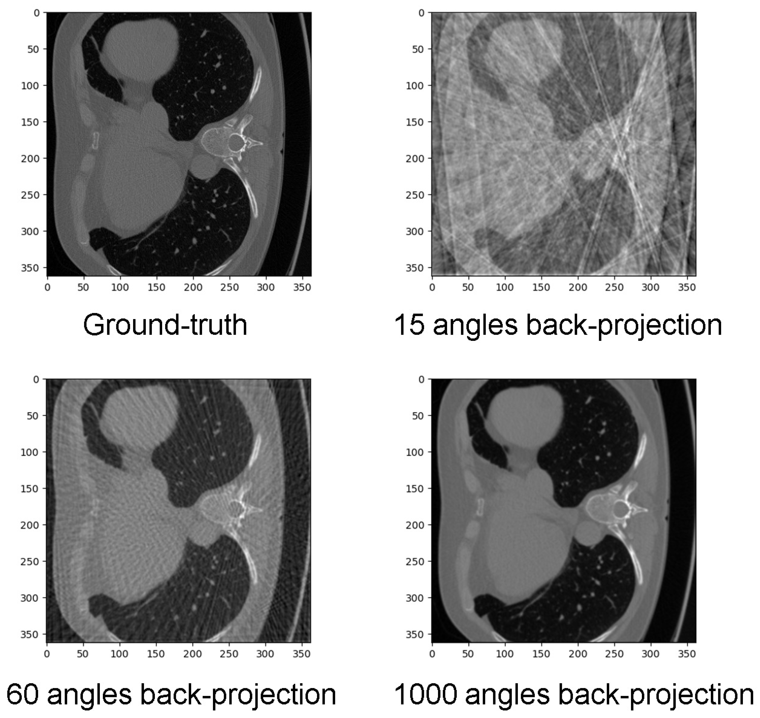
Sparse angle computed tomography reconstruction is a technique used to reconstruct CT images from a limited set of projections. The number of projections used to reconstruct the image is an important factor that determines the quality of the reconstruction. When using a limited number of projections, there is a trade-off between the quality of the reconstructed image and the computational complexity of the reconstruction algorithm. If too few projections are used, the reconstructed image may be noisy and contain artifacts. On the other hand, using too many projections may increase the computational complexity of the reconstruction algorithm and lead to longer reconstruction times. In the case of sparse-angle CT reconstruction, using 60 angles for the projections is a common practice because it strikes a balance between image quality and computational complexity. This number of projections has been found to provide a good balance between noise reduction and preserving image details while still being computationally feasible. It is also a compromise between the typical 180-degree scan of a full CT scan and the more limited number of projections used in other sparse-angle CT reconstruction techniques. Many related works also use 60-angle projection data for sparse-angle CT reconstruction, such as [10,38].

Traditional industrial CT mainly uses a cone beam X-ray source and an X-ray flat panel detector to collect circular trajectory projection data by rotating the measured object on a rotating stage and uses the FDK reconstruction algorithm to reconstruct the three-dimensional volume of the measured object [39]. This form of scanning needs to use manual or six-axis robots to fix the measured object on a rotating platform before scanning the measured object and then performs scanning and imaging steps. There are two major drawbacks to this form of scanning. First, because the size of the measured object is limited by the X-ray flat panel detector, and the flat panel detector is generally unable to produce a larger size, the size of the measured object is often limited. Second, the use of manual or six-axis robots to fix the measured object and then scan the form greatly reduces the detection efficiency, which makes the CT non-destructive testing link in the actual production process often adopt the method of random sampling inspection. Unfortunately, random sampling inspection cannot guarantee a 100% pass rate for the measured product.

Our proposed structure can be easily integrated into the production line, which greatly improves the efficiency of non-destructive testing and brings a 100% pass rate for the measured products. In addition, since line array X-ray detector can have a very long size, the size of the measured object will no longer be subject to strict restrictions. Through the deployment of deep-learning neural networks, many fewer projections are needed for reconstruction through a well-trained neural network, and it greatly shortens the reconstruction time and provides a solution for real-time CT.

2. Hardware Design

2.1. System Structure

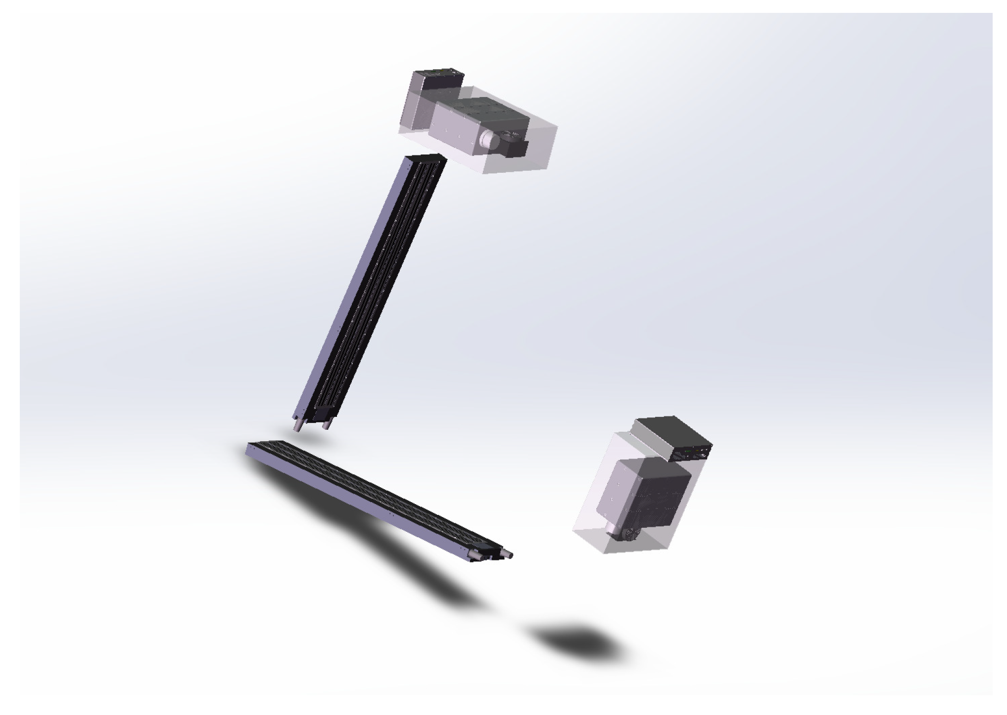
The main parts of our CT system include a fan beam X-ray source and a linear X-ray detector. The X-ray detector we use is the X-scan ME Series produced by Detection Technology, and the X-ray source is the IXS1203 microfocus X-ray source produced by VJX-ray; the voltage range of the X-ray source tube is 40–120 kV, the tube current range is 0.05–0.3 mA and the focal size is 50 μm. The total cost of our proposed system is about USD 700,000.

In order to reduce the space needed between the scanner, we combine these two main parts into a pair of detection module. As is shown in Figure 1, the imaging modules in group 1 and in group 2 are distributed staggered, and the circumferential distance is 105 degrees.

The detector specifications of our system are illustrated in

Table 1. The detector specifications.

Feature	Value
Detection method	Photon counting
Crystal thickness	2 mm
Detector element pitch	0.8 mm
Detector element binning	1 × 1 (0.8 mm pitch)
Active area length	1229 mm (1536 pixels)
Energy range	20 to 160 keV
Line speed	4 m/min to 96 m/min
Counting period	0.5 ms to 100 ms
Dead time	10 $\mathsf{\mu }$s
Energy bins (channels)	Up to 128
Pixel dynamic range/energy bin	16 bits per bin

; inspected slice numbers in each object can be calculated based on those parameters:

$$K=\frac{L}{S·(P+T)}$$

(1)

In Equation (1), K refers to the inspected slice numbers in each measured object on the conveyor belt, L(m) refers to measured object length, S(m/s) refers to line speed, P(s) refers to counting period and T(s) refers dead time. To make sure the inspected slices in different measured objects are aligned, e.g., the location of slice 1 in measured object 1 is consistent with the location of slice 1 in measured object 2. Only in this way will projections in different angles of each slice be guaranteed to locate in the same plane, which avoids distortion during the reconstruction process. The frame rate for our real-time imaging can be calculated as follows:

$$FPS=\frac{1}{(P+T)}$$

(2)

Imaging quality can be modified by controlling the number of energy bins:

$$Q=A·w·b·Pr$$

(3)

where Q refers to the quality of projections, A refers to Active area length, w refers to Detector element width, b refers to energy bins and Pr refers to Pixel dynamic range. Projection quality determines the quality of reconstructed slices.

The equipment is based on the principle of CT slice imaging, with the difference being that the X-ray source and detector through the spiral array arranged with the detected work-piece around the motion direction for the work-piece that is panning on the conveyor belt; whenever one of the interfaces passes through all the detection modules, the reconstruction process is completed.

In parallel beam X-ray CT reconstruction, when the detector rotates 360${}^{\circ }$ around the object, the projection data generated by each ray is measured twice, and each projection data point in the range of 180${}^{\circ }$ to 360${}^{\circ }$ is a repeated acquisition of projected data in the range of 0${}^{\circ }$ to 180${}^{\circ }$, which is redundant, so the detector only needs to rotate 180${}^{\circ }$ to provide sufficient projection data for image reconstruction. 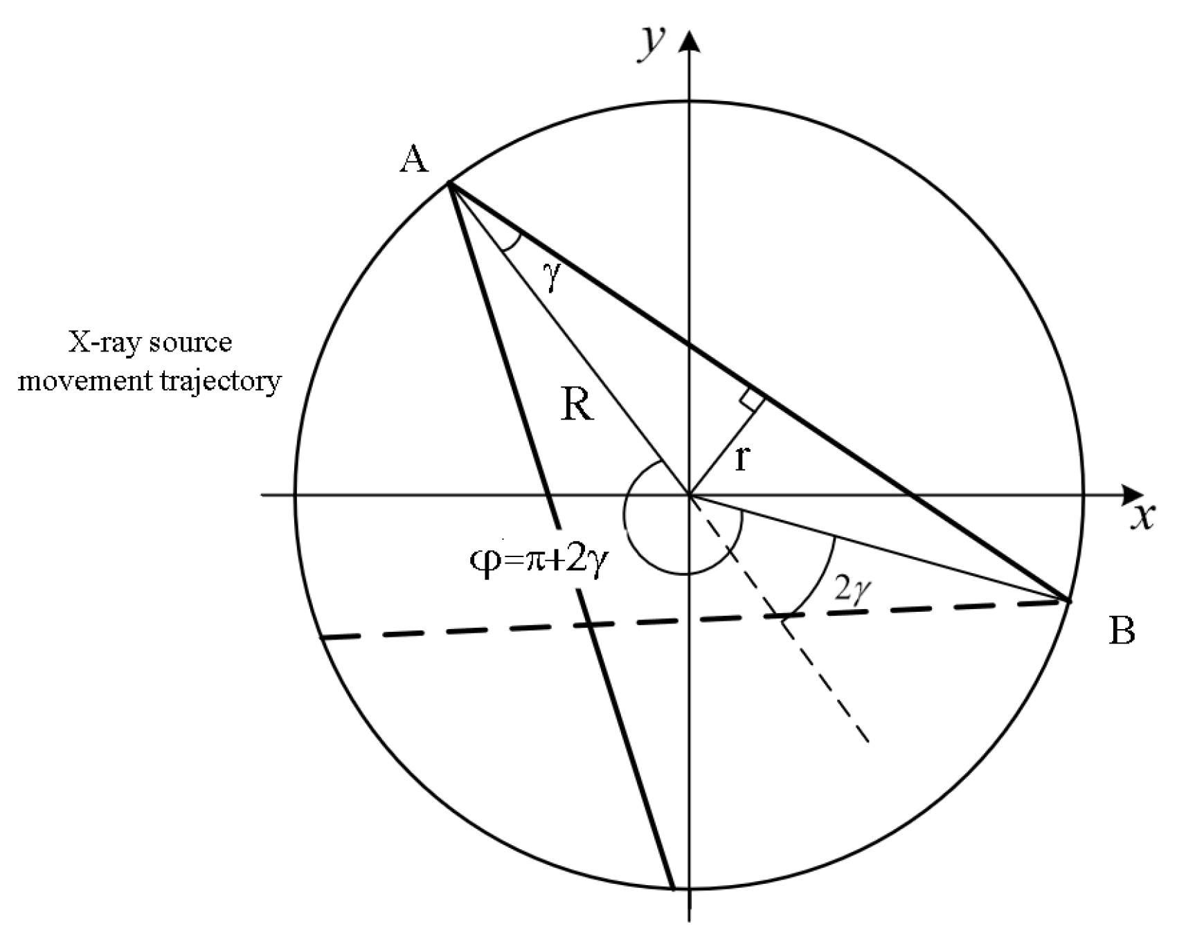Similarly, in the sector beam X-ray CT reconstruction, the projection data generated by each ray when the detector rotates 360${}^{\circ }$ has also been measured twice, and in the actual data acquisition process, there is no need to perform a 360${}^{\circ }$ full scan, and the scanning angle can be less than 360${}^{\circ }$, which is called short scanning. As is shown in the Figure 2, when the sector beam light source rotating around a circular trajectory rotates from position A to position B, the first X-ray of the position A sector beam coincides with the last ray of the position B sector beam, and each point in the field of view is covered by rays distributed in an angle range of at least 180${}^{\circ }$, from which the minimal rotation angle $\phi$ can be derived:

$$\phi =\pi +2·arcsin\left(\frac{r}{R}\right)$$

(4)

where r is the radius of the field of view, and R is the distance between the source and the axis of rotation. One slice of volume is complete when all the needed projections are back projected. In our system, r is around 280 mm, and R is around 1661 mm. Based on Equation (4), the minimal rotation angle is 199.41 degrees. We designated the distribution angle of all the detection module as 206.5 degrees for calculation convenience.

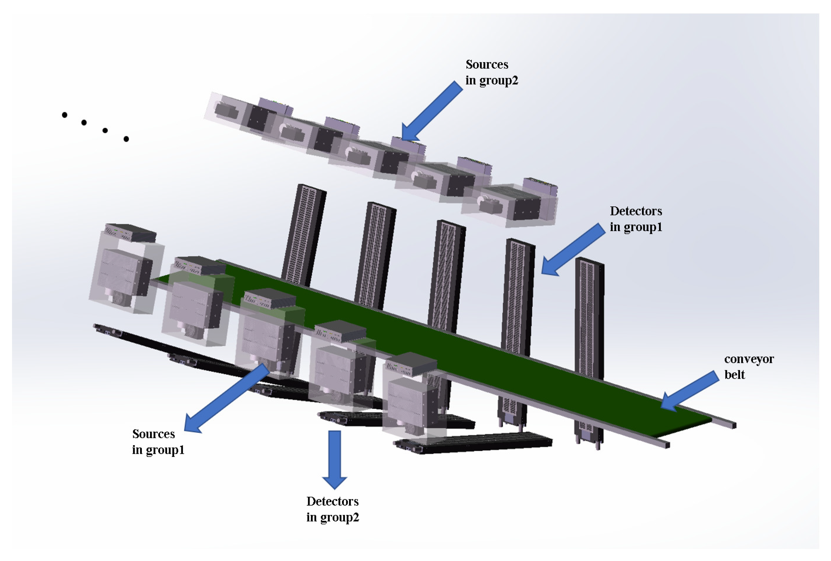
As is shown in Figure 3, the X-ray source and X-ray detector in the first group are aligned in pairs, and correspondingly, the X-ray source and the X-ray detector in the second group are aligned in pairs as well. The distance between two adjacent sources or two adjacent detectors in each group along the direction of the conveyor belt is 735 mm, and the angle between them is 3.5 degrees around the circumferential direction of the conveyor.

In the reconstruction process, it is necessary to obtain a sufficient angle of projection data in order to ensure the image quality of the reconstructed slices. The device obtains cross-section projection data at 60 different angles for slice image reconstruction through the arrangement of 60 pairs of X-ray sources and detectors. The circumferential angle interval between each group of light source detectors is 3.5${}^{\circ }$, and the total detection angle is 206.5${}^{\circ }$. In order to reduce the minimum distance between each pair of X-ray source and detector and make the equipment more compact as a whole, a space-interleaved arrangement is adopted.

From 0${}^{\circ }$ to 101.5${}^{\circ }$, X-ray sources and detectors are arranged every 3.5${}^{\circ }$, and a total of 30 pairs are arranged, forming the first group. From 105${}^{\circ }$ to 206.5${}^{\circ }$, other pairs of X-ray sources and detectors are arranged every 3.5${}^{\circ }$ for a total of 30 pairs as well, forming a second group, and the two groups add up to a total of 60 pairs of X-ray sources and detectors; the overall view and side view of the system is shown in Figure 4.

With the development of modern industry, industrial CT plays a major role in non-destructive testing and reverse engineering. The results of non-destructive testing of products using industrial CT show that industrial CT technology has high detection sensitivity for various common defects such as porosity, inclusion, pinhole, shrink hole, and delamination. It can accurately determine the size of these defects and locate their position in the object as well. Compared with other conventional non-destructive testing technologies, the spatial and density resolution of industrial CT technology is less than 0.5%, the imaging size accuracy is high, and it is not limited by the type and geometry of the work-piece material. It can generate three-dimensional images of material defects, which is of great research and application value in the detection of defects such as structural dimensions, material uniformity, micro-pore rate and overall micro-cracks, inclusions, porosity and abnormally large grains in the work-piece to be inspected.

2.2. Data Processing

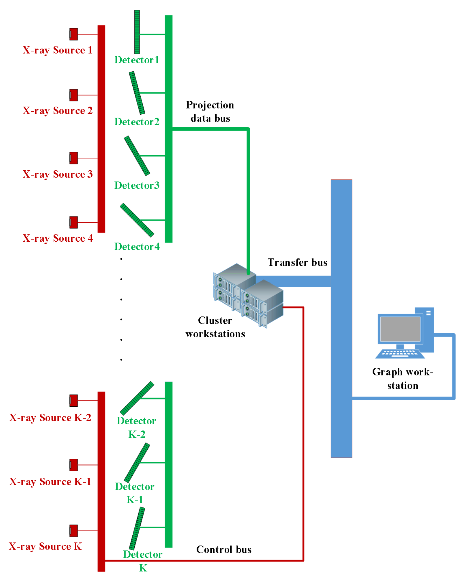
The data collected by the detectors were sent to the cluster workstation with GPU for processing. The X-ray intensity data after attenuation was divided by the X-ray intensity data without any attenuation. Projections were acquired after this process. The data transmission network is shown in Figure 5.

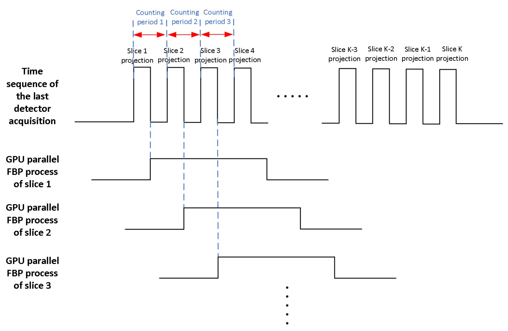
Usually, a rotary CT scanner acquires all the projection data after one rotational scan and carries out the reconstruction procedure. Before the projection data of the next slice was collected, the FBP reconstruction procedure in GPU has already finished. Therefore, the parallel computing power of GPUs is not well tapped, and the low computing efficiency is not suitable for real-time imaging. In our proposed structure, after projection data in the last angle were acquired by the detector, the reconstruction procedure in this slice of interest was executed. By the time the last projection of the next slice of interest was collected, which is much shorter than the imaging algorithm, the reconstruction procedure of this new slice of interest was executed in parallel in the GPU. Thus, the parallel computing power of GPUs is well exerted. Time sequence of data processing is shown in Figure 6.

In our implementation we preferred to create a continuous reconstruction scheme where the filtered and back-projected slice enter into the system as soon as a new series of projections were read in. In this way, we have a continuous stream of projections that were received from the detectors and a continuous stream of reconstructed slices that was sent to the image processing stage. In such a way, objects can be continuously processed even if they only have a small gap between them on the conveyor. We implemented the FBP algorithm on the cluster workstation with the GPU to perform the filtered back-projection after the projections were read by detectors. The reconstruction results were then sent to the graphics workstation for post processing by deep learning.

3. Reconstruction Algorithms

3.1. Filtered Back Projection

The formation and reconstruction of CT images are mathematically described as the radon transform and the radon inverse transform, respectively [40,41]. To put it simply, the radon transform is a mathematical representation of the process of forming a CT image by X-ray scanning of an object, while the radon inverse transformation describes a mathematical method of reconstructing CT projection data and transforming them into an object image. The radon inverse transformation is actually a two-dimensional Fourier inverse transformation mathematically, and its mathematical expression is as follows [42]:

$$\begin{array}{cc}\hfill f(x,y)& ={\int }_{-\infty }^{\infty }{\int }_{-\infty }^{\infty }F(u,v)e^{j2\pi (ux+vy)}dudv\hfill \\ \hfill & ={\int }_0^{2\pi }{\int }_0^{\infty }F(\omega cos\theta ,\omega sin\theta )e^{j2\pi \omega (xcos\theta +ysin\theta )}\omega d\omega d\theta \hfill \end{array}$$

(5)

Due to the large amount of calculation and long time consumption of the two-dimensional Fourier inverse transformation, the specific implementation method of the computer for the radon inverse transformation is mainly the back-projection method, and the back-projection method is divided into direct back-projection method and the filtered back-projection method. Averaging the error during the smear, error caused by interpolation and star-like artifacts caused by the overlay of the back projection bring the 1/r effect. The following convolutional relationship exists between the refactored image $f_b(x,y)$ and the real original image f(x,y):

$$f_b(x,y)=f(x,y)·\frac{1}{r}$$

(6)

In Equation (6), 1/r is also known as a fuzzy factor. The most commonly used method of removing the 1/r effect is the filtered and re-projected method.

As can be seen from Equation (6) above, 1/r is convolved with the original image, and after transitioning to the frequency domain by the Fourier transform, it will become a multiplicative relationship, which means that it is easier to process directly at frequency. In the frequency domain, r is called the weight factor, which is actually equivalent to a filter. Method 1 only takes three steps to remove the influence of the blur factor and reconstruct the original image:

• Step1: Perform a two-dimensional Fourier transform on the reconstructed image $f_b(x,y)$ to obtain $F_b(x,y)$;
• Step2: Multiply $F_b(x,y)$ by the filter r in the frequency domain;
• Step3: Take r ×$F_b(x,y)$ for a two-dimensional Fourier inverse transformation to obtain the original figure f(x,y).

Equation (5) is the mathematical expression for Method 1.

Method 2 of first back-projecting and then filtering requires the use of 2 two-dimensional Fourier transforms, which needs large amount of computation. This kind of method is not particularly ideal. The filtering and back-projection method, as the name suggests, is a reconstruction method of filtering first and then re-projecting. The specific steps are as follows:

• Step1: Transform the projection signals at each angle into one-dimensional Fourier;
• Step2: Filter all projected signals in the frequency domain, that is, multiplied by the weight factor r;
• Step3: Transform inversely all filtered signals in one dimension and restore to the time domain;
• Step4: back-project and finally superimpose each filtered projection signal.

The advantage of this method is that the two-dimensional Fourier transforms are changed into two one-dimensional Fourier transforms, and the calculation speed is greatly improved. One-dimensional Fourier transform of the projection of $\rho$ is:

$$G(\omega ,\theta )={\int }_{-\infty }^{\infty }g(\rho ,\theta )e^{-j2\pi \omega \rho }d\rho$$

(7)

The mathematical expression for Method 2 is [42]

$$f(x,y)={\int }_0^{2\pi }{\left[{\int }_{-\infty }^{\infty }\omega G(\omega ,\theta )e^{j2\pi \omega \rho }d\omega \right]}_{\rho =xcos\theta +ysin\theta }d\theta$$

(8)

The core problem of filtering and in-projection becomes how to choose a suitable filter r. Filter r in mathematics is an idealized filter function that does not exist in reality, so only an approximate filter function can be designed to replace the role of filter r. R-L filter function and S-L filter function are commonly used filter functions. To eliminate the ringing effect caused by the window function, the smoothing window function is used:

$$h\left(\omega \right)=\left\{\begin{array}{cc}c+(c-1)cos\frac{2\pi \omega }{M},& 0\le \omega \le (M-1)\\ 0,& other\end{array}\right.$$

(9)

This slope filter function is called the Hamming window when c = 0.54 and Hann window when c = 0.5 [42].

Basically, filtered back projection (FBP) is a convolution operation on the basis of the back projection. The specific process of using filter inversion to reconstruct the image is to first convolve the original data obtained by the detector with a filter function to obtain the projection function of convolution in each direction and then to reverse project them from all directions, that is, to distribute them evenly to each matrix element according to its original path and to obtain the CT value of each matrix element after superposition. Then, after appropriate processing, the tomographic image of the scanned object can be obtained, and the convolutional projection can eliminate the edge sharpness effect caused by the simple back projection. The filter function compensates for the high-frequency components in the projection and reduces the density of the projection center and ensures that the edges of the reconstructed image are clear and the internal distribution is uniform. As the number of projections increases, the quality of the reconstruction is increased significantly.

The ground-truth images were selected from an open-source data set LoDoPaB-CT [43]. The projection data were acquired from helical thoracic CT scans of 812 individuals with the X-ray tube peak voltages ranging from 120 kV to 140 kV and tube current ranging from 40 mA to 627 mA with a mean of 222.1 mA. The image reconstruction was performed with different filters, depending on the manufacture of the scanner. All reconstructed images have a resolution of 362 pixels × 362 pixels on a domain of size 26 cm × 26 cm. We used an open-access Python package Astra-toolbox [44] to simulate the forward-projecting process in different projection numbers. We performed FBP algorithm to reconstruct the CT images from those simulated projections to compare the reconstruction quality. It can be seen from Figure 7 that the effect on reconstruction quality with the increment in projection number.

3.2. Deep Convolutional Neural Network Design

3.2.1. Network Structure

As is shown in Figure 7, if the process of image reconstruction is regarded as a process of solving a system of equations, and the gray value of each pixel on the picture is an unknown, then the number of equations must be greater than the number of unknowns to make the system of equations have a definite solution. For a 512 × 512 CT image, there are 262,144 unknowns, and if a line array detector with 1536 detection elements is used, the projected data for each angle will introduce 1536 equations, and then at least 171 angles of projection data will be required to have a definitive solution for this system of equations. Not to mention that, to get a sharper image, you need more equations to increase the constraints. In practical engineering applications, the FBP reconstruction algorithm needs to obtain at least 360 projection data points within 360${}^{\circ }$ to perform clear image reconstruction. In our system architecture, the X-ray source and detector remain stationary, and the measured objects are translated through multiple groups of detection units composed of X-ray sources and detectors. At least 360 groups of light sources and detectors are required if it is reconstructed according to the traditional FBP algorithm, which makes the hardware cost too high and the volume of the equipment too large. To make our design practical, it is essential to reduce the number of X-ray sources and detectors. Consequently, the CT reconstruction process becomes an ill-posed question trying to obtain the solution with insufficient parameters. The FBP reconstruction result contains many artifacts, especially streaking artifacts, and it is obvious that image with those artifacts cannot meet the requirements of industrial inspection. Typically, some post-processing approaches such as denoising were applied to reduce those artifacts. Recent works have successfully used convolutional neural networks such as U-Net to solve this kind of problem. Chen Hu et al. presented a novel approach for enhancing the quality of low-dose computed tomography (LDCT) images using a residual encoder–decoder convolutional neural network (RED-CNN). The primary aim was to improve the diagnostic quality of LDCT scans while reducing the radiation exposure to patients [45]. Jin Kyong Hwan et al. proposed a novel deep learning approach that leverages the power of CNNs to learn an end-to-end mapping from the degraded images to their high-quality counterparts. The key contribution of this work is the development of a highly efficient and accurate CNN architecture which is specifically designed to tackle various inverse problems in imaging [46]. Yang Qingsong et al. presented a novel approach to denoise low-dose computed tomography (LDCT) images using a generative adversarial network (GAN) that incorporates Wasserstein distance and perceptual loss. The primary goal was to enhance the quality of LDCT images while minimizing radiation exposure to patients [47]. Ronneberger Olaf et al. proposed a novel convolutional neural network (CNN) architecture called U-Net for biomedical image segmentation tasks. The U-Net architecture consists of a contracting path and an expansive path, which allows the network to learn both high-level context and low-level detailed information [48]. Kawauchi Keisuke et al. proposed a CNN architecture that is specifically designed to process and analyze FDG PET/CT images. The CNN model extracts relevant features from the input images and classifies patients based on the presence or absence of abnormal FDG uptake, which is indicative of disease. The proposed system can potentially assist radiologists in making more accurate and timely diagnoses [49]. Protonotarios Nicholas E et al. proposed a modified U-Net architecture that can learn effective lesion segmentation with only a few annotated training examples. The few-shot learning approach enables the model to generalize well to unseen PET/CT images, reducing the need for large amounts of labeled data. The proposed U-Net model leverages the strengths of both PET and CT imaging modalities to achieve more accurate and robust segmentation of lung cancer lesions [50].

Basically, we were trying to train an end-to-end neural network to acquire clean reconstruction results out of the noisy FBP reconstruction results from sparse-view projection data. In our design, the sparse-view projection data was acquired through 60 angles which were evenly distributed within 180${}^{\circ }$. The structure of our sparse-view reconstruction network is shown in Figure 8.

Several details of the network are as follows:

• Down-sampling: U-net extracts the features of the input image through max-pooling and two-dimensional convolution operations. In the process of down-sampling, the size of the image feature map continues to shrink, and the number of feature channels continues to increase, which means that more local details of the image are extracted.
• Up-sampling: De-convolution, more precisely transposed convolution, operations were used to gradually restore ground-truth from features. It can be understood as an inverse process of down-sampling; during this process, image features are gradually restored. In order to ensure that the feature scale change during the up-sampling process is symmetrical with the down-sampling process, the kernel size and padding of transposed convolution are variable.
• Feature fusion: Before every up-sampling process, input features are fused with the features in feature extraction part at the same feature scale. Using the abstract features encoded earlier to restore to the original size, U-Net employs a completely different way of feature fusion: concatenation. U-net concatenates features together in the channel dimension to form thicker features. When recovering the down-sampling data, the feature scale changes, and inevitably there is information loss. At this time, the role of feature fusion is highlighted. Feature fusion plays a role in supplementing information. U-Net integrates features of different scales, while the jump connection ensures that the features recovered from the up-sampling will not be very rough. Some research found that jump connections can make the network minimizer flatter by visualizing the loss landscape, resulting in less sensitivity to new data and stronger generalization capabilities [51].
• Residual Learning: Inspired by the good generalization performance of the residual network [52], we added a skip connection between input image and output image. Pixels of the input and output image are added linearly, which means that the network essentially learns the difference between input image and output image. The vanishing gradient problem during training can be effectively avoided with this approach.

Our model was designed in Python using PyTorch framework. All the experiments run on Linux system with 24G NVIDIA RTX3090 GPU, Xeon Platinum 8157 CPU @ 3GHz and 86G RAM. The specifications of our proposed network are shown in the following

Table 2. Specifications of the network.

Layer	Input Channels	Output Channels	Kernel Size	Stride	Padding
Conv0	1	64	3	1	‘same’
Conv1	64	64	3	1	‘same’
Conv2	64	64	3	1	‘same’
Max pooling0	64	64	2	2	0
Conv3	64	128	3	1	‘same’
Conv4	128	128	3	1	‘same’
Max pooling1	128	128	2	2	1
Conv5	128	256	3	1	‘same’
Conv6	256	256	3	1	‘same’
Max pooling2	256	256	2	2	1
Conv7	256	512	3	1	‘same’
Conv8	512	512	3	1	‘same’
Max pooling3	512	512	2	2	0
Conv9	512	1024	3	1	‘same’
Conv10	1024	1024	3	1	‘same’
Conv_trans0	1024	512	2	2	0
Conv11	1024	512	3	1	‘same’
Conv12	512	512	3	1	‘same’
Conv_trans1	512	256	3	2	1
Conv13	512	256	3	1	‘same’
Conv14	256	256	3	1	‘same’
Conv_trans2	256	128	3	2	1
Conv15	256	128	3	1	‘same’
Conv16	128	128	3	1	‘same’
Conv_trans3	128	64	2	2	0
Conv17	128	64	3	1	‘same’
Conv18	64	64	3	1	‘same’
Conv19	64	1	3	1	‘same’

. The code of constructing and training this model is avaliable at https://github.com/vintagewtj/sparse-view-CT-reconstruction (accessed on 20 December 2022).

3.2.2. Dataset

The dataset comes from LoDoPaB-CT [43]. This dataset crops all included images to consistently 362 × 362 pixels. Consequently, the number of weight parameters in our proposed model is greatly reduced and the network is easier to train. One of the big challenges of training a network with good performance is acquiring a high quality dataset for training. Unfortunately, industrial CT datasets are usually not available given that patent protection is involved. In this case, we tried to train the network using open-source medical datasets and assess the performance using the industrial CT image acquired in our laboratory. Several methods have been applied to improve the generalization of the model, including data augmentation and L2 regularization.

Data augmentation is effective to improve the desired invariance and robustness properties of the network. Since we want to train the reconstruction network using a medical dataset and apply it to industrial images, data augmentation can be a good trick. We randomly flipped the input images and the corresponding target images, either in the X or Y direction or in both directions.

The model that uses L2 regularization is called ridge regression. Loss function in this model would be [53]:

$$min\frac{1}{2m}{{\sum }_{i=1}^m\left(f\left(x\right)-y^{\left(i\right)}\right)}^2+\lambda {∥w∥}_2^2$$

(10)

where $\lambda$ is the weight coefficient of the L2 regularization. The larger the $\lambda$, the stronger the restriction on the weight vector. In the process of the L2 regularization, it is generally inclined to make the weights in the network as small as possible. A model with small parameter values is relatively simple and has great adaption to different datasets. L2 regularization avoids the phenomenon of overfitting to a certain extent. It can be imagined that for a linear regression equation, if the parameters are large, then as long as the data are offset a little, it will have a great impact on the result, but if the parameters are small enough, a little more data offset will not affect the result, and the anti-interference ability is strong.

3.3. Reconstruction Quality Assessment

In this initial study, for the FBP, Hann filters were used as, we mentioned before. For the post-processing approach (FBP + U-Net), we used a U-Net architecture with five scales. We trained it using the proposed dataset by minimizing the mean squared error loss with the Adam algorithm for a maximum of 20 epochs with batch size 16. Additionally, we used a learning rate of $1\times {10}^{-5}$, and the weight parameter of L2 regularization is $1\times {10}^{-7}$. Training loss and test loss during the training are shown in Figure 9. The model with the highest mean peak signal-to-noise ratio (PSNR) on the test set was selected during training. Reconstructed samples are shown in Figure 10. Region of interest (ROI) of sample 1 is show in Figure 11, and we can see that artifacts caused by undersampling were clearly reduced.

To validate the reconstruction quality of our proposed deep learning approach, we provide reference reconstructions and quantitative results for the standard filtered back-projection (FBP) and a learned post-processing method (FBP + U-Net).

The mean squared error (MSE) is a widely employed metric in the realm of machine learning and statistical modeling, particularly for regression tasks. It serves as a measure of the average squared difference between the true and predicted values, quantifying the model’s performance in terms of accuracy and error. With its differentiable and continuous nature, MSE allows for gradient-based optimization techniques, making it a popular choice for various algorithms such as linear regression, support vector machines, and neural networks. MSE can be expressed by the following formula:

$$MSE=\frac{1}{mn}{{\sum }_{i=1}^{m-1}{\sum }_{j=0}^{n-1}\left[I(i,j)-K(i,j)\right]}^2$$

(11)

We used the PSNR to evaluate the reconstruction quality. Peak signal-to-noise ratio (PSNR) is an engineering term that expresses the ratio of the maximum possible power of a signal to the destructive noise power that affects the accuracy of its representation. Since many signals have a very wide dynamic range, the PSNR is often expressed in logarithmic decibel units. It can be written as follows:

$$PSNR=10·{log}_{10}\left(\frac{MA{X}_I^2}{MSE}\right)=20·{log}_{10}\left(\frac{MA{X}_I}{\sqrt{MSE}}\right)$$

(12)

$MA{X}_I$ is the maximum numeric value that represents the color of an image point. As we can see from the formula, the smaller the MSE, the larger the PSNR, and the better image quality.

Structural similarity (SSIM) is used to calculate the similarity of two input images. One of them is a ground truth, the other is a reconstructed image, and SSIM can be used as a measure of quality. The mathematical definition of SSIM is

$$\begin{array}{c}\hfill SSIM={\left|l\right(x,y\left)\right|}^{\alpha }{\left|c\right(x,y\left)\right|}^{\beta }{\left|s\right(x,y\left)\right|}^{\alpha \gamma }\end{array}$$

(13)

In Equation (13):

$$l(x,y)=\frac{2{\mathsf{\mu }}_x{\mathsf{\mu }}_y+c_1}{{\mathsf{\mu }}_x^2+{\mathsf{\mu }}_y^2+c_1}$$

(14)

$$c(x,y)=\frac{2{\sigma }_{xy}+c_2}{{\sigma }_x^2+{\sigma }_y^2+c_2}$$

(15)

$$s(x,y)=\frac{{\sigma }_{xy}+c_3}{{\sigma }_x{\sigma }_y+c_3}$$

(16)

l(x,y) is the brightness component, c(x,y) is a contrast component, s(x,y) is the structural component. ${\mathsf{\mu }}_x$ and ${\mathsf{\mu }}_y$ represent the means of x, y, and ${\sigma }_x$ and ${\sigma }_y$ represent the standard deviation of x, y, respectively. ${\sigma }_{xy}$ represents the covariance of x and y.

Table 3. Reconstruction metrics for test dataset.

	FBP	Epoch 1	Epoch 5	Epoch 10	Epoch 15	Epoch 20
MSE	$4.13\times {10}^{-4}$±$2.87\times {10}^{-8}$	$2.58\times {10}^{-4}$±$2.06\times {10}^{-8}$	$6.96\times {10}^{-5}$±$2.41\times {10}^{-9}$	$4.79\times {10}^{-5}$±$1.72\times {10}^{-9}$	$4.44\times {10}^{-5}$±$1.62\times {10}^{-9}$	$4.29\times {10}^{-5}$±$1.68\times {10}^{-9}$
PSNR	29.22 ± 4.87 dB	31.39 ± 4.46 dB	37.23 ± 6.10 dB	39.03 ± 7.48 dB	39.40 ± 7.85 dB	39.59 ± 7.99 dB
SSIM	0.69 ± $3.9\times {10}^{-3}$	0.79 ± $4.6\times {10}^{-3}$	0.92 ± $1.6\times {10}^{-3}$	0.94 ± $1.5\times {10}^{-3}$	0.94 ± $1.3\times {10}^{-3}$	0.95 ± $1.4\times {10}^{-3}$

depicts the obtained results in terms of the MSE, PSNR and SSIM metrics during the training compared with the FBP results; 100 samples in test dataset were used to calculate those metrics. As it can be observed, in the process of MSE reduction, the FBP+U-net approach outperforms the classical FBP reconstructions by a margin of 10 dB in PSNR, and the SSIM improved by 38%. This demonstrates that our proposed reconstruction method achieves good performance in the test dataset.

In order to compare with other approaches existing in the state of the art, we compare our trained network with the traditional FBP algorithm [37], SIRT iterative algorithm [54], Residual network (Res-net) [52] and Learned Primal-Dual network (LPD-net) [55] in Figure 12. Projected data with the same number of projecting angles are used as input. The evaluation metrics were shown in

Table 4. Reconstruction metrics comparison of different methods with 60 angles projection.

	FBP	SIRT	Res-net	LPD-net	U-net
MSE	$4.13\times {10}^{-4}$	$8.99\times {10}^{-4}$	$1.59\times {10}^{-4}$	$1.56\times {10}^{-3}$	$4.29\times {10}^{-5}$
PSNR	29.22 dB	27.64 dB	34.65 dB	25.41 dB	39.59 dB
SSIM	0.69	0.69	0.90	0.72	0.95

, we can find that the reconstruction results of our trained network have better reconstruction quality at the same number of projections compared to other methods.

To verify the generalization of the network on industrial CT, we used CT images of spectral interferometer for verification, which was acquired by the Shimadzu CT instrument at the tube voltage of 200 kV and the tube current of 70 ${\mathsf{\mu }}_A$. Figure 13 shows the reconstruction comparison of industrial CT.

Table 5. Reconstruction metrics for industrial data.

	FBP in 60 Angles	FBP+U-net
MSE	$7.75\times {10}^{-4}$	$1.09\times {10}^{-4}$
PSNR	31.04 dB	39.52 dB
SSIM	0.76	0.95

shows that the model also has great performance on industrial data. We recorded the change of different metrics in both test dataset and industrial data during the training process in Figure 14.

All the reconstructed slices are stacked to present the effect of the 3D reconstruction, and we compare the 3D reconstruction results before and after using the trained neural network to correct the undersampling reconstruction results in Figure 15. It can been seen from the figure that the artifacts resulted from undersampling have been greatly reduced using our proposed neural network.

Experimental results show that our proposed reconstruction method also has great performance on our acquired industrial CT image, which means our network has great generalization. Therefore, the image reconstruction quality of proposed system can meet the demand of industrial non-destructive testing.

3.4. Time Consumption Analysis

As is shown in Figure 16, we selected different slices of the spectral interferometer for reconstruction to calculate the reconstruction time consumption after these slices pass through the detector scan plane. Time consumption is mainly composed of two parts: sparse-view FBP process in the cluster workstation and the post-processing in the graphics workstation. We calculated the reconstruction time consumption of the two steps on the tested slices, and the result is shown in

Table 6. Time consumption of different slices.

	Slice1	Slice2	Slice3	Slice4	Slice5	Slice6	Average
FBP/s	0.004	0.004	0.004	0.004	0.005	0.004	0.004
Post-processing/s	0.125	0.123	0.123	0.124	0.123	0.123	0.124
Total/s	0.129	0.127	0.127	0.128	0.128	0.127	0.128

.

In our proposed reconstruction solution, the trained network is stored in the graphics workstation. Sparse-view projections acquired by the detectors were sent to the GPU in the cluster workstation for FBP reconstruction at first, and then the reconstructed images were sent to the network as inputs; the final reconstructed images were acquired as the outputs of the network. We can see from Table 5 that the time consumption is mainly determined by post-processing time; in our Nvidia RTX3060 GPU, time consumption of the whole procedure is around 0.128 s. We have reason to believe that time consumption can be decreased using a more advanced GPU. By changing the interval between inspected objects on the conveyor belt, our system can meet the demands of real-time imaging. The gap between inspected objects should satisfy the following formula:

$$g>S·R_T$$

(17)

In Equation (17), g refers to gap between inspected objects, S refers to line speed of the convey belt, $R_T$ refers to the reconstruction time we estimated. The readout time of the detector is crucial for the whole imaging process, if the readout time is too long, projections in the detectors cannot be guaranteed to come from the same slice, which makes an enormous alignment error.

4. Discussion and Conclusions

In our simulation, the slices of interest of the inspected object were successfully constructed in a short time by the CT structure we proposed. The inspection part is highly integrated into the whole production line so that the quality inspection has been simplified and the production cycle has been greatly shortened. Meanwhile, a sufficient quantity of X-ray detectors and the deep-learning reconstruction method make sure that the quality of the reconstructed slices satisfies the needs of defect detection.

The micro-focal X-ray source used in our system has a focal size of 50 $\mathsf{\mu }$m, and it can meet the need for clear imaging on detectors with pixel dimensions in the hundreds of $\mathsf{\mu }$m range. In order to control the cost of the entire system, we currently choose a detector with a pixel size of 0.8 mm, i.e., 800 $\mathsf{\mu }$m. Since the measured objects are roughly halfway between the X-ray source and X-ray detector, the magnification is about 2. Theoretically, the maximum spatial resolution is up to 400 $\mathsf{\mu }$m (half the pixel size of the detector), which is sufficient for non-destructive testing of some large internal defects. For some smaller defects, we can choose detectors with smaller pixel size to cope with higher detection needs, and the common pixel sizes of the detectors on the market are 0.1 mm, 0.2 mm, 0.4 mm, and 0.8 mm.

By adjusting the key parameters of the system, the real-time imaging frame rate and image quality are variable. Slices of comprehensive structure and dangerous sections can be scanned with higher frame rates and imaging quality, while some irrelevant slices can be scanned with lower frame rates and imaging quality. Computing power is effectively saved in this arrangement. Some other solutions can also apply in our system, such as inspecting the object in the region of interest so that the reconstruction time can be decreased [56].

This is the first time training the network using a medical dataset and applying it to industrial CT reconstruction. The medical CT data can be viewed as the source domain, and the acquired industrial CT data can be viewed as the target domain. Transfer learning can greatly reduce the training time and deployment cycle by applying the pre-trained model from the source domain to the target domain.

In a further study, we will focus on reducing the needed projection number for reconstruction by optimizing the deep-learning reconstruction network and applying the knowledge of transfer learning [57]. In this way, the number of X-ray sources and detectors can be further reduced, and the system structure complexity and the cost will be reduced as well.

With the guarantee of imaging quality and imaging speed, our proposed system provides an ideal solution for the sorting, grading, quality inspection, material analysis and optimization of complex manufacturing processes in recycling, food processing, mining and other process industries. It can also be applied in the field of security as well.

Our proposed system can significantly increase the speed and accuracy of inspection in production processes, and it is convenient to be integrated into production lines. Evaluation metrics and inspection images are updated in real time, and the quality of each product can be verified.

References

1. Roentgen, W.C. On a new kind of rays. CA Cancer J. Clin. 1972, 22, 153–157. [Google Scholar] [CrossRef] [PubMed]
2. Hounsfield, G.N. Computerized transverse axial scanning (tomography): Part 1. Description of system. Br. J. Radiol. 1973, 46, 1016–1022. [Google Scholar] [CrossRef] [PubMed]
3. Yang, M.; Duan, S.; Duan, J.; Wang, X.; Li, X.; Meng, F.; Zhang, J. Extra projection data identification method for fast-continuous-rotation industrial cone-beam CT. J. X-ray Sci. Technol. 2013, 21, 467–479. [Google Scholar] [CrossRef] [PubMed]
4. Yan, G.; Tian, J.; Zhu, S.; Dai, Y.; Qin, C. Fast cone-beam CT image reconstruction using GPU hardware. J. X-ray Sci. Technol. 2008, 16, 225–234. [Google Scholar]
5. Giudiceandrea, F.; Enrico, U.; Enrico, V. A high speed CT scanner for the sawmill industry. In Proceedings of the 17th International Non Destructive Testing and Evaluation of Wood Symposium, Sopron, Hungary, 14–16 September 2011. [Google Scholar]
6. Ursella, E.; Federico, G.; Marco, B. A Fast and Continuous CT scanner for the optimization of logs in a sawmill. In Proceedings of the 8th Conference on Industrial Computed Tomography (iCT 2018), Wels, Austria, 6–9 February 2018; Volume 2. [Google Scholar]
7. Robb, R.A.; Hoffman, E.A.; Sinak, L.J.; Harris, L.D.; Ritman, E.L. High-speed three-dimensional X-ray computed tomography: The dynamic spatial reconstructor. Proc. IEEE 1983, 71, 308–319. [Google Scholar] [CrossRef]
8. Wu, W.; Niu, C.; Ebrahimian, S.; Yu, H.; Kalra, M.; Wang, G. AI-Enabled Ultra-Low-Dose CT Reconstruction. arXiv 2021, arXiv:2106.09834. [Google Scholar]
9. Sidky, E.Y.; Lorente, I.; Brankov, J.G.; Pan, X. Do CNNs solve the CT inverse problem? IEEE Trans. Biomed. Eng. 2020, 68, 1799–1810. [Google Scholar] [CrossRef]
10. Han, Y.; Ye, J.C. Framing U-Net via deep convolutional framelets: Application to sparse-view CT. IEEE Trans. Med. Imaging 2018, 37, 1418–1429. [Google Scholar] [CrossRef] [Green Version]
11. Zhang, H.; Li, L.; Qiao, K.; Wang, L.; Yan, B.; Li, L.; Hu, G. Image prediction for limited-angle tomography via deep learning with convolutional neural network. arXiv 2016, arXiv:1607.08707. [Google Scholar]
12. Survarachakan, S.; Pelanis, E.; Khan, Z.A.; Kumar, R.P.; Edwin, B.; Lindseth, F. Effects of Enhancement on Deep Learning Based Hepatic Vessel Segmentation. Electronics 2021, 10, 1165. [Google Scholar] [CrossRef]
13. Choi, B.-H.; Hwang, D.; Kang, S.-K.; Kim, K.-Y.; Choi, H.; Seo, S.; Lee, J.-S. Accurate Transmission-Less Attenuation Correction Method for Amyloid-β Brain PET Using Deep Neural Network. Electronics 2021, 10, 1836. [Google Scholar] [CrossRef]
14. Dao-Ngoc, L.; Du, Y.C. Generative Noise Reduction in Dental Cone-Beam CT by a Selective Anatomy Analytic Iteration Reconstruction Algorithm. Electronics 2019, 8, 1381. [Google Scholar] [CrossRef] [Green Version]
15. Chen, H.; Zhang, Y.; Zhang, W.; Liao, P.; Li, K.; Zhou, J.; Wang, G. Low-dose CT via convolutional neural network. Biomed. Opt. Express 2017, 8, 679. [Google Scholar] [CrossRef] [Green Version]
16. Xu, L.; Ren, J.S.; Liu, C.; Jia, J. Deep convolutional neural network for image deconvolution. Adv. Neural Inf. Process. Syst. 2014, 27. Available online: https://www.lxu.me/mypapers/dcnn_nips14.pdf (accessed on 29 March 2023).
17. Van Tiggelen, R. In search for the third dimension: from radiostereoscopy to three-dimensional imaging. JBR-BTR 2002, 85, 266–270. [Google Scholar]
18. Thomas, A.M.; Banerjee, A.K. The History of Radiology; OUP Oxford: New York, NY, USA, 2013. [Google Scholar]
19. Webb, S. From the Watching of Shadows: The Origins of Radiological Tomography; CRC Press: Boca Raton, FL, USA, 1990. [Google Scholar]
20. Kevles, B. Naked to the Bone: Medical Imaging in the Twentieth Century; Rutgers University Press: Chicago, IL, USA, 1997. [Google Scholar]
21. Moore, T.; Vanderstraeten, D.; Forssell, P. Determination of BGA structural defects and solder joint defects by 3D X-ray laminography. In Proceedings of the 2001 8th International Symposium on the Physical and Failure Analysis of Integrated Circuits, Singapore, 13 July 2001; pp. 146–150. [Google Scholar] [CrossRef]
22. Thompson, A.; Leach, R. Introduction to Industrial X-ray Computed Tomography. In Industrial X-ray Computed Tomography; Springer: New York, NY, USA, 2018; pp. 1–23. [Google Scholar] [CrossRef]
23. Gilboy, W.; Foster, J. Industrial applications of computerized tomography with X-and gamma-radiation. In Research Techniques in Nondestructive Testing; Academic Press: London, UK, 1982; Volume 6, pp. 255–287. [Google Scholar]
24. Reimers, P.; Goebbels, J. New possibility of nondestructive evaluation by X-ray computed tomography. Mater. Eval. 1983, 41, 732–737. [Google Scholar]
25. Kress, J.; Feldkamp, L. X-ray tomography applied to NDE of ceramics. In Proceedings of the ASME 1983 International Gas Turbine Conference and Exhibit, Phoenix, AZ, USA, 27–31 March 1983. [Google Scholar] [CrossRef] [Green Version]
26. Oster, R. Computed Tomography as a Don-Destructive Test Method for Fiber Main Rotor Blades in Development, Series and Maintenance; Gesellschaft für Standortbetreiberdienste: Bremen, Germany, 1997. [Google Scholar]
27. Liu, C.; Wang, R.R.; Ho, I.; Kong, Z.J.; Williams, C.; Babu, S.; Joslin, C. Toward online layer-wise surface morphology measurement in additive manufacturing using a deep learning-based approach. J. Intell. Manuf. 2022, 1–17. [Google Scholar] [CrossRef]
28. Elhefnawy, M.; Ragab, A.; Ouali, M.S. Fault classification in the process industry using polygon generation and deep learning. J. Intell. Manuf. 2022, 33, 1531–1544. [Google Scholar] [CrossRef]
29. Ma, Z.; Li, Y.; Huang, M.; Huang, Q.; Cheng, J.; Tang, S. Automated real-time detection of surface defects in manufacturing processes of aluminum alloy strip using a lightweight network architecture. J. Intell. Manuf. 2022, 1–17. [Google Scholar] [CrossRef]
30. Nogueira, M.L.; Greis, N.P.; Shah, R.; Davies, M.A.; Sizemore, N.E. Machine learning classification of surface fracture in ultra-precision diamond turning using CSI intensity map images. J. Manuf. Syst. 2022, 64, 657–667. [Google Scholar] [CrossRef]
31. Xu, C.; Wang, J.; Tao, J.; Zhang, J.; Zheng, P. A knowledge augmented deep learning method for vision-based yarn contour detection. J. Manuf. Syst. 2022, 63, 317–328. [Google Scholar] [CrossRef]
32. Cramer, A.; Hecla, J.; Wu, D.; Lai, X.; Boers, T.; Yang, K.; Moulton, T.; Kenyon, S.; Arzoumanian, Z.; Krull, W. Stationary computed tomography for space and other resource-constrained environments. Sci. Rep. 2018, 8, 14195. [Google Scholar] [CrossRef] [PubMed] [Green Version]
33. Zhang, T.; Xing, Y.; Zhang, L.; Jin, X.; Gao, H.; Chen, Z. Stationary computed tomography with source and detector in linear symmetric geometry: Direct filtered backprojection reconstruction. Med. Phys. 2020, 47, 2222–2236. [Google Scholar] [CrossRef] [PubMed]
34. Cao, H.; Yunxiang, L.; Chang, T.; Cui, Z.; Zheng, H. Stationary Real Time CT Imaging System and Method Thereof. U.S. Patent 10743826, 18 August 2020. [Google Scholar]
35. Spronk, D.; Luo, Y.; Inscoe, C.R.; Lee, Y.Z.; Lu, J.; Zhou, O. Evaluation of carbon nanotube X-ray source array for stationary head computed tomography. Med. Phys. 2021, 48, 1089–1099. [Google Scholar] [CrossRef]
36. Qian, X.; Tucker, A.; Gidcumb, E.; Shan, J.; Yang, G.; Calderon-Colon, X.; Sultana, S.; Lu, J.; Zhou, O.; Spronk, D.; et al. High resolution stationary digital breast tomosynthesis using distributed carbon nanotube X-ray source array. Med. Phys. 2012, 39, 2090–2099. [Google Scholar] [CrossRef] [Green Version]
37. Crowther, R.A.; DeRosier, D.; Klug, A. The reconstruction of a three-dimensional structure from projections and its application to electron microscopy. Proc. R. Soc. Lond. A Math. Phys. Sci. 1970, 317, 319–340. [Google Scholar]
38. Lee, M.; Kim, H.; Kim, H.J. Sparse-view CT reconstruction based on multi-level wavelet convolution neural network. Phys. Medica 2020, 80, 352–362. [Google Scholar] [CrossRef]
39. Feldkamp, L.A.; Davis, L.C.; Kress, J.W. Practical cone-beam algorithm. JOSA A 1984, 1, 612–619. [Google Scholar] [CrossRef] [Green Version]
40. Deans, S.R. The Radon Transform and Some of Its Applications; Courier Corporation: Chelmsford, MA, USA, 2007. [Google Scholar]
41. Natterer, F. The Mathematics of Computerized Tomography; SIAM: Philadelphia, PA, USA, 2001. [Google Scholar]
42. Gonzales, R.; Woods, R. Digital Image Processing, 4th ed.; Pearson Education Limited: New York, NY, USA, 2018. [Google Scholar]
43. Leuschner, J.; Schmidt, M.; Baguer, D.O.; Maass, P. LoDoPaB-CT, a benchmark dataset for low-dose computed tomography reconstruction. Sci. Data 2021, 8, 109. [Google Scholar] [CrossRef]
44. Van Aarle, W.; Palenstijn, W.J.; Cant, J.; Janssens, E.; Bleichrodt, F.; Dabravolski, A.; De Beenhouwer, J.; Batenburg, K.J.; Sijbers, J. Fast and flexible X-ray tomography using the ASTRA toolbox. Opt. Express 2016, 24, 25129–25147. [Google Scholar] [CrossRef] [Green Version]
45. Chen, H.; Zhang, Y.; Kalra, M.K.; Lin, F.; Chen, Y.; Liao, P.; Zhou, J.; Wang, G. Low-dose CT with a residual encoder-decoder convolutional neural network. IEEE Trans. Med. Imaging 2017, 36, 2524–2535. [Google Scholar] [CrossRef]
46. Jin, K.H.; McCann, M.T.; Froustey, E.; Unser, M. Deep convolutional neural network for inverse problems in imaging. IEEE Trans. Image Process. 2017, 26, 4509–4522. [Google Scholar] [CrossRef] [Green Version]
47. Yang, Q.; Yan, P.; Zhang, Y.; Yu, H.; Shi, Y.; Mou, X.; Kalra, M.K.; Zhang, Y.; Sun, L.; Wang, G. Low-dose CT image denoising using a generative adversarial network with Wasserstein distance and perceptual loss. IEEE Trans. Med. Imaging 2018, 37, 1348–1357. [Google Scholar] [CrossRef]
48. Ronneberger, O.; Fischer, P.; Brox, T. U-net: Convolutional networks for biomedical image segmentation. In Proceedings of the International Conference on Medical Image Computing and Computer-Assisted Intervention, Munich, Germany, 5–9 October 2015. [Google Scholar] [CrossRef] [Green Version]
49. Kawauchi, K.; Furuya, S.; Hirata, K.; Katoh, C.; Manabe, O.; Kobayashi, K.; Watanabe, S.; Shiga, T. A convolutional neural network-based system to classify patients using FDG PET/CT examinations. BMC Cancer 2020, 20, 227. [Google Scholar] [CrossRef] [Green Version]
50. Protonotarios, N.E.; Katsamenis, I.; Sykiotis, S.; Dikaios, N.; Kastis, G.A.; Chatziioannou, S.N.; Metaxas, M.; Doulamis, N.; Doulamis, A. A few-shot U-Net deep learning model for lung cancer lesion segmentation via PET/CT imaging. Biomed. Phys. Eng. Express 2022, 8, 025019. [Google Scholar] [CrossRef]
51. Lu, J.; Tong, K.Y. Visualized insights into the optimization landscape of fully convolutional networks. arXiv 2019, arXiv:1901.08556. [Google Scholar]
52. He, K.; Zhang, X.; Ren, S.; Sun, J. Deep residual learning for image recognition. In Proceedings of the IEEE Conference on Computer Vision and Pattern Recognition, Las Vegas, NV, USA, 27–30 June 2016. [Google Scholar]
53. Goodfellow, I.; Bengio, Y.; Courville, A. Deep Learning; MIT Press: Cambridge, MA, USA, 2016. [Google Scholar]
54. Andersen, A.H.; Kak, A.C. Simultaneous algebraic reconstruction technique (SART): A superior implementation of the ART algorithm. Ultrason. Imaging 1984, 6, 81–94. [Google Scholar] [CrossRef]
55. Adler, J.; Öktem, O. Learned primal-dual reconstruction. IEEE Trans. Med. Imaging 2018, 37, 1322–1332. [Google Scholar] [CrossRef] [Green Version]
56. Reimers, P.; Kettschau, A.; Goebbels, J. Region-of-interest (ROI) mode in industrial X-ray computed tomography. NDT Int. 1990, 23, 255–261. [Google Scholar] [CrossRef]
57. Pan, S.J.; Yang, Q. A survey on transfer learning. IEEE Trans. Knowl. Data Eng. 2009, 22, 1345–1359. [Google Scholar] [CrossRef]
Figure 1. Two adjacent imaging modules.
Electronics 12 01815 g001
Figure 2. Derivation of the minimum scanning angle of the sector beam.
Electronics 12 01815 g002
Figure 3. Scenograph of the system.
Electronics 12 01815 g003
Figure 4. Overall view and side view of the system. (a) Overall view of the system; (b) side view of the system.
Electronics 12 01815 g004
Figure 5. Data transmission network.
Electronics 12 01815 g005
Figure 6. Time sequence of data processing.
Electronics 12 01815 g006
Figure 7. FBP results with different projection numbers.
Electronics 12 01815 g007
Figure 8. U-Net structure.
Electronics 12 01815 g008
Figure 9. Train loss and test loss. (a) train loss; (b) test loss.
Electronics 12 01815 g009
Figure 10. Dataset sample reconstruction.
Electronics 12 01815 g010
Figure 11. Comparison in region of interest.
Electronics 12 01815 g011
Figure 12. Comparison of different reconstruction methods.
Electronics 12 01815 g012
Figure 13. Industrial data reconstruction. (a) Ground-truth; (b) FBP in 60 angles; (c) FBP+U-net.
Electronics 12 01815 g013
Figure 14. Metrics changes in training process. (a) MSE; (b) PSNR; (c) SSIM.
Electronics 12 01815 g014
Figure 15. Three-dimensional reconstruction result: (a) 3D reconstruction before performing neural network correction; (b) 3D reconstruction after performing neural network correction.
Electronics 12 01815 g015
Figure 16. Slices for time consumption test.
Electronics 12 01815 g016