

Federated Learning for Medical Imaging Segmentation via Dynamic Aggregation on Non-IID Data Silos


Abstract
:1. Introduction
- A new dynamic aggregation scheme was designed to enhance the stability and quality of segmentation results. We dynamically adjusted the client’s weight during training instead of fixing a constant weight according to the number of samples or the average distribution.
- We proposed a distillation regularization loss function, i.e., using Kullback–Leibler divergence to guide the local generator model. It prevents essential parameters of the global generator model from significantly changing while tuning the global generator model on client-side local data.
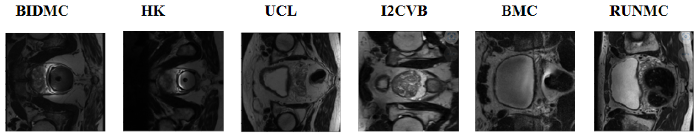
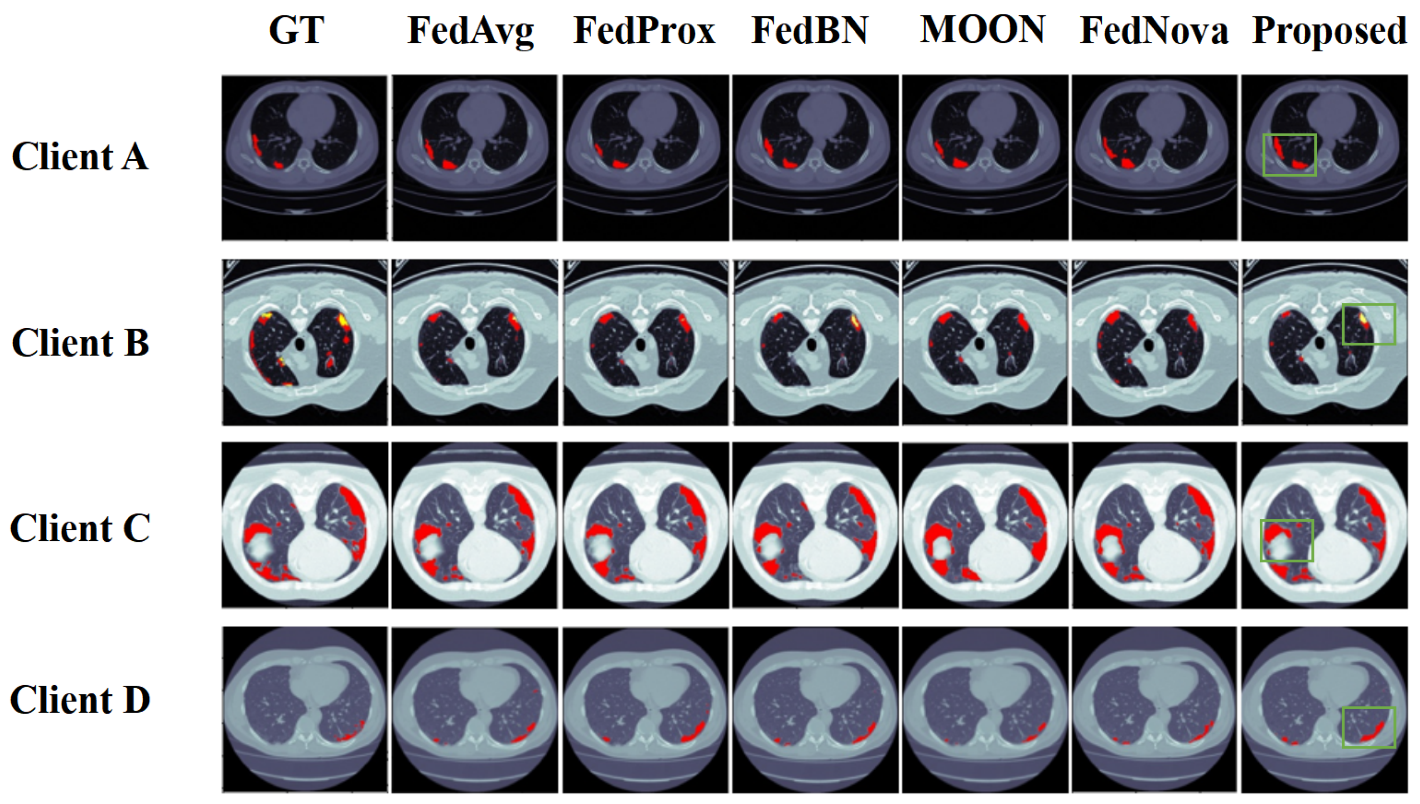
- We considered the effectiveness of our framework in both supervised and semi-supervised scenarios and conducted an experimental analysis on four heterogeneous COVID-19 segmentation datasets and three heterogeneous prostate MRI datasets. Both comparative and ablation experiments show that our method is more stable and efficient.
2. Related Works and Motivation
2.1. Federated Learning
2.2. Generative Adversarial Network
2.3. Motivation
3. Methods
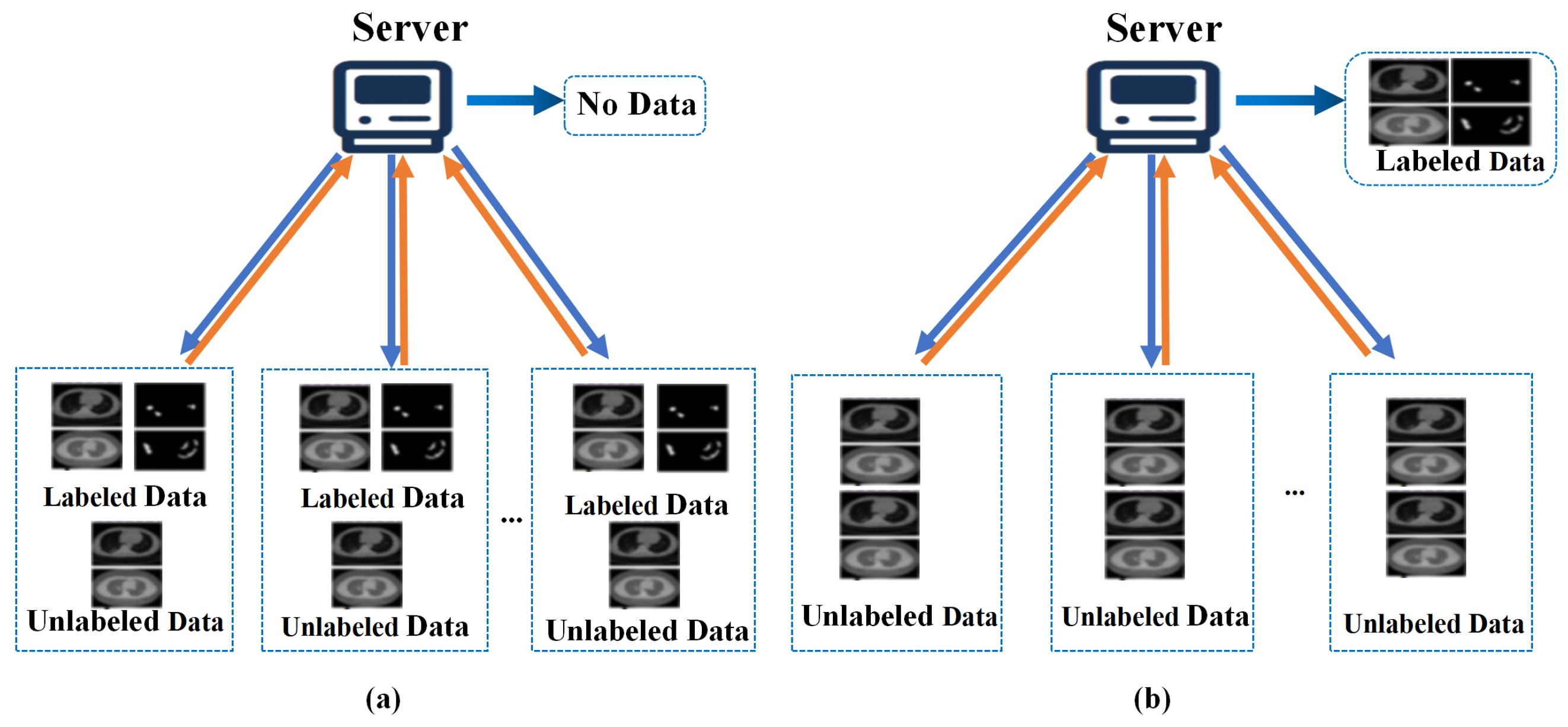
3.1. Problem-Setting
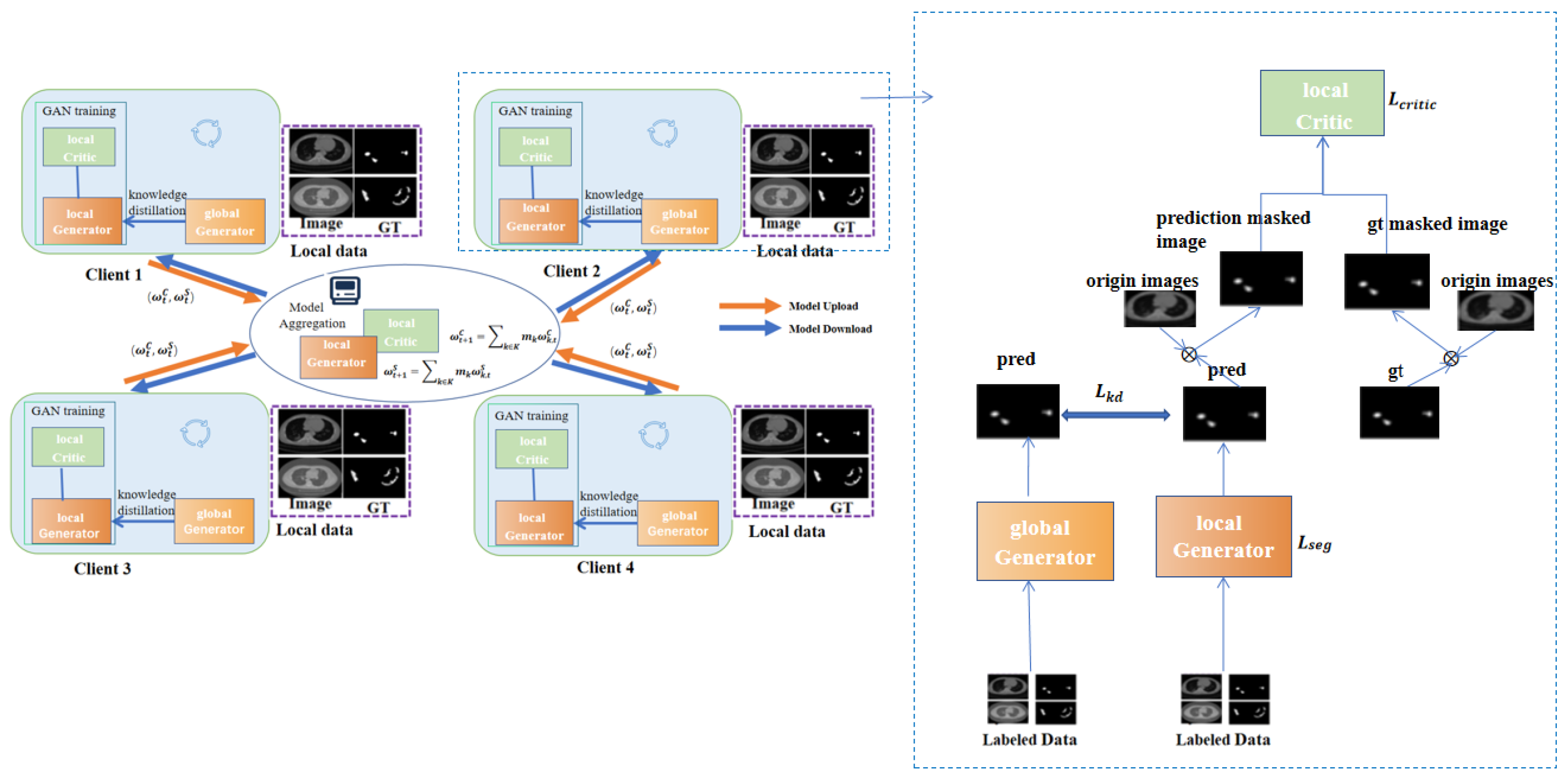
3.2. MixFedGAN-Supervised
| Algorithm 1 Training procedure of the proposed MixFedGAN |
|
3.3. Dynamic Aggregation
3.4. Knowledge Distillation in MixFedGAN
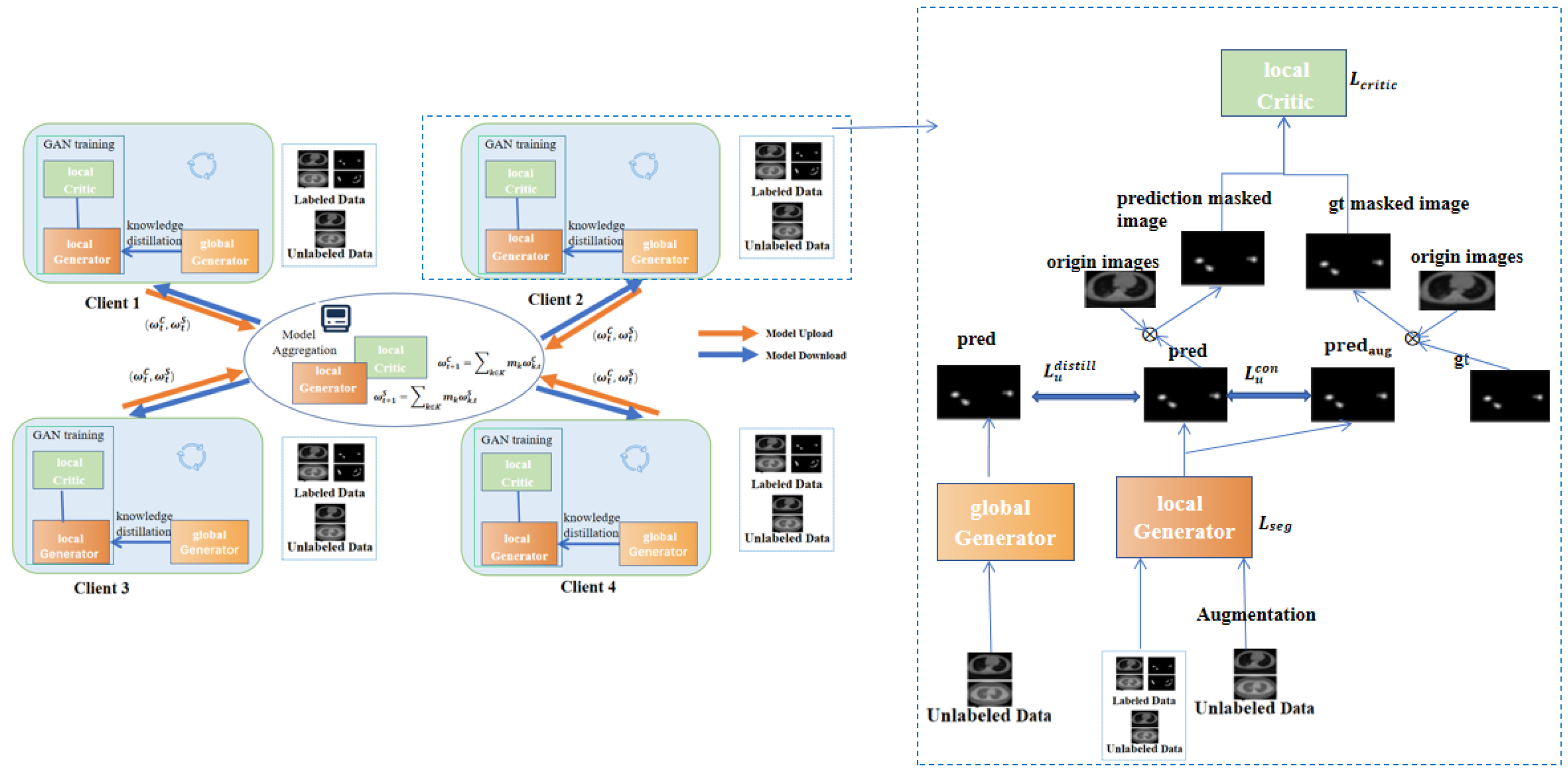
3.5. MixFedGAN-Semi-Supervised
4. Experiments
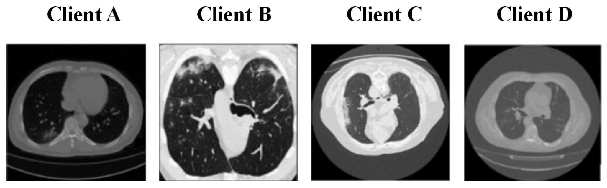
4.1. Dataset
4.2. Experimental Setup and Evaluation Metrics
4.3. Comparison Experiments and Ablation Study
4.4. Dealing with Semi-Supervised Setting
5. Discussion
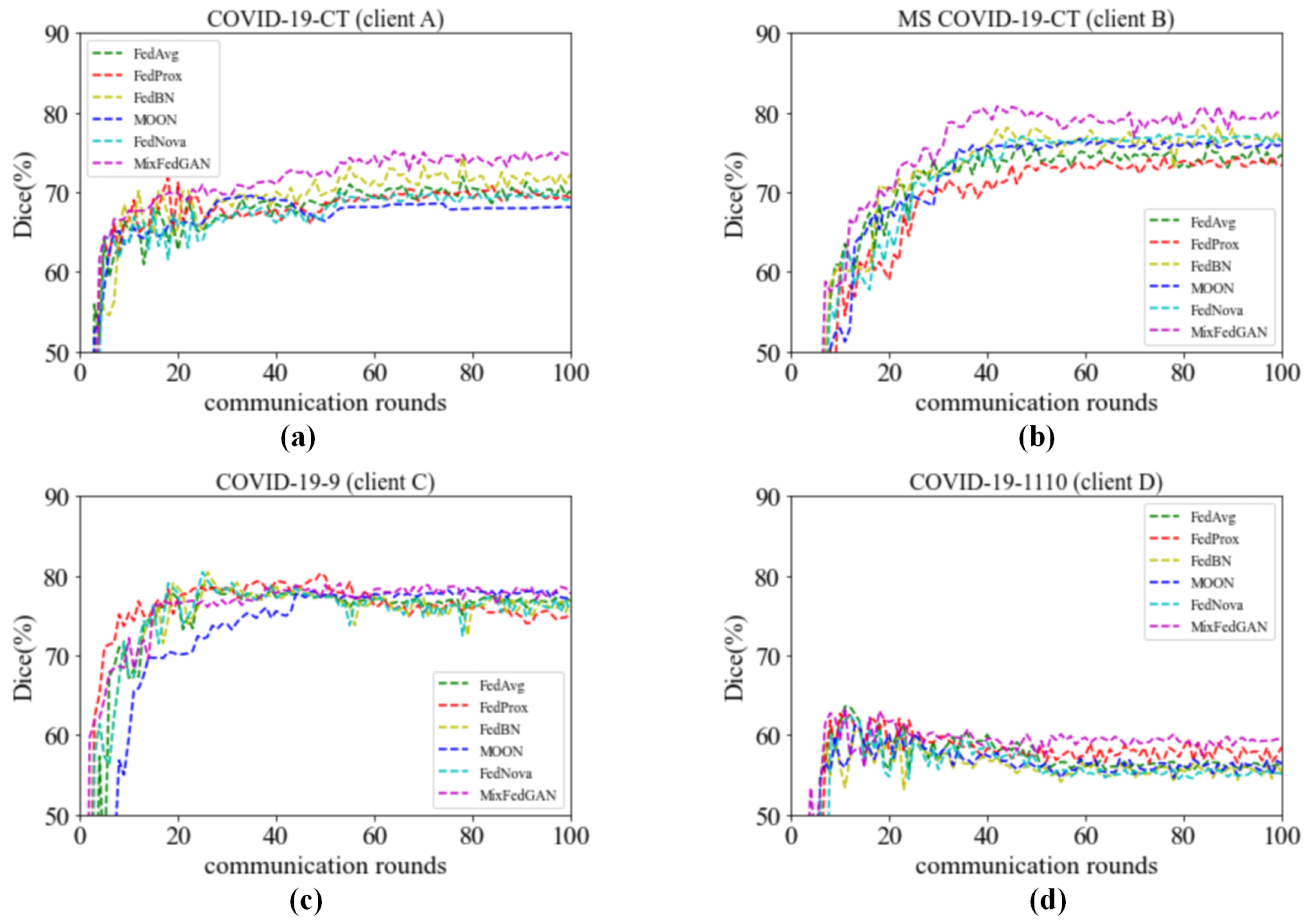
5.1. Convergence Analysis
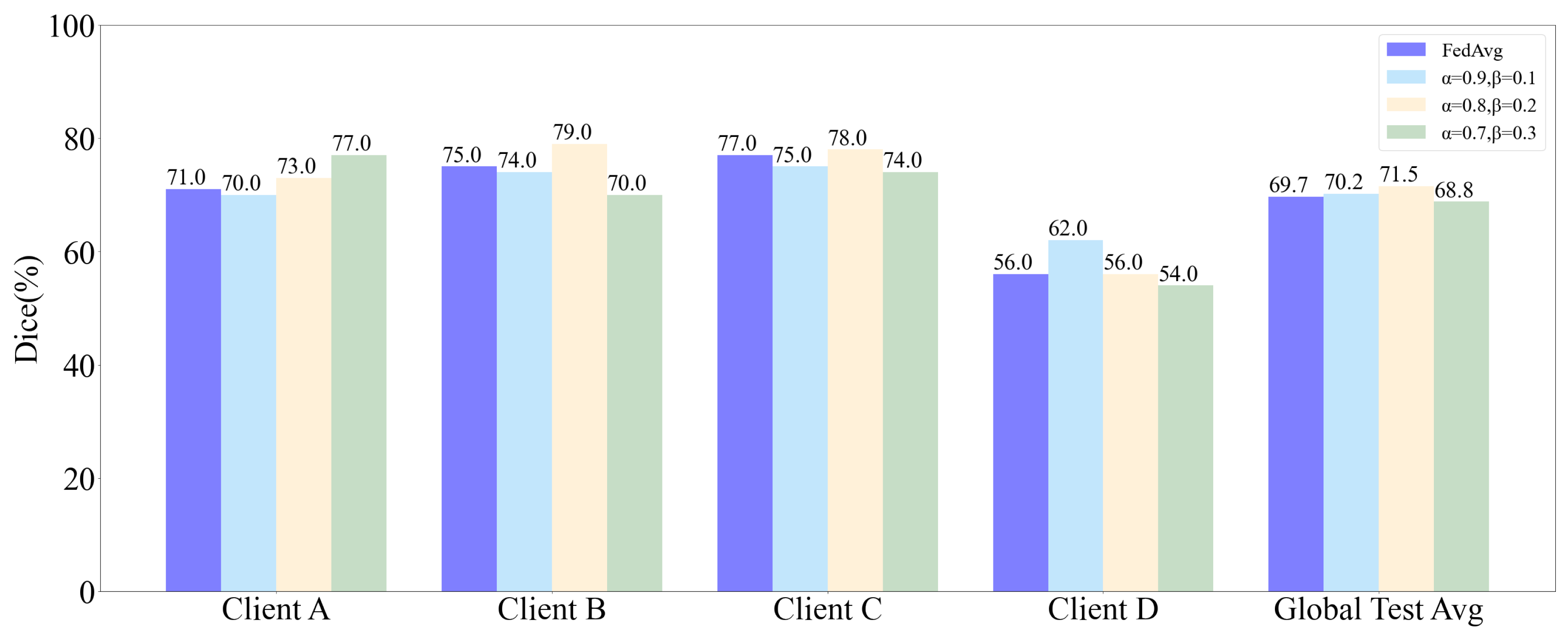
5.2. Influence of and
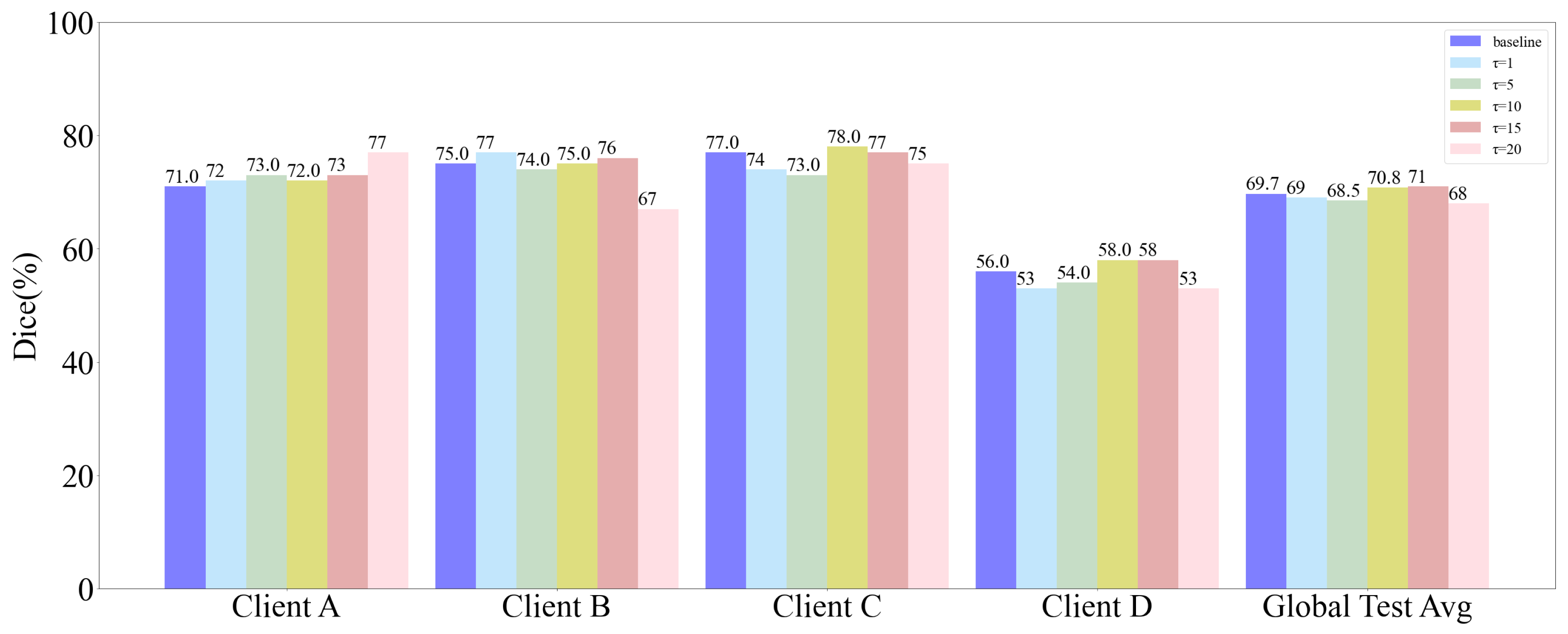
5.3. Influence of Distillation Temperature
5.4. Computation and Communication Cost
6. Conclusions
Author Contributions
Funding
Institutional Review Board Statement
Informed Consent Statement
Data Availability Statement
Conflicts of Interest
References
- Zhou, T.; Li, L.; Bredell, G.; Li, J.; Unkelbach, J.; Konukoglu, E. Volumetric memory network for interactive medical image segmentation. Med. Image. Anal. 2023, 83, 102599. [Google Scholar] [CrossRef] [PubMed]
- Liu, X.; Yuan, Q.; Gao, Y.; He, K.; Wang, S.; Tang, X.; Tang, J.; Shen, D. Weakly supervised segmentation of COVID19 infection with scribble annotation on CT images. Pattern Recognit. 2022, 122, 108341. [Google Scholar] [CrossRef]
- He, J.; Zhu, Q.; Zhang, K.; Yu, P.; Tang, J. An evolvable adversarial network with gradient penalty for COVID-19 infection segmentation. Appl. Soft Comput. 2021, 113, 107947. [Google Scholar] [CrossRef]
- Liu, X.; Guo, Z.; Cao, J.; Tang, J. MDC-net: A new convolutional neural network for nucleus segmentation in histopathology images with distance maps and contour information. Comput. Biol. Med. 2021, 135, 104543. [Google Scholar] [CrossRef] [PubMed]
- Yang, Q.; Liu, Y.; Chen, T.; Tong, Y. Federated machine learning: Concept and applications. ACM Trans. Intell. Syst. Technol. 2019, 10, 1–19. [Google Scholar] [CrossRef]
- Xu, J.; Glicksberg, B.S.; Su, C.; Walker, P.; Bian, J.; Wang, F. Federated Learning for Healthcare Informatics. J. Healthc. Inform. Res. 2019, 5, 1–19. [Google Scholar] [CrossRef]
- Qayyum, A.; Ahmad, K.; Ahsan, M.A.; Al-Fuqaha, A.; Qadir, J. Collaborative Federated Learning for Healthcare: Multi-Modal COVID-19 Diagnosis at the Edge. IEEE Open J. Comput. Soc. 2022, 3, 172–184. [Google Scholar] [CrossRef]
- Dou, Q.; So, T.Y.; Jiang, M.; Liu, Q.; Vardhanabhuti, V.; Kaissis, G.; Li, Z.; Si, W.; Lee, H.H.C.; Yu, K.; et al. Federated deep learning for detecting COVID-19 lung abnormalities in CT: A privacy-preserving multinational validation study. NPJ Digit. Med. 2021, 4, 1–11. [Google Scholar] [CrossRef]
- Sarma, K.V.; Harmon, S.; Sanford, T.; Roth, H.R.; Xu, Z.; Tetreault, J.; Xu, D.; Flores, M.G.; Raman, A.G.; Kulkarni, R.; et al. Federated learning improves site performance in multicenter deep learning without data sharing. J. Am. Med. Inform. Assoc. 2021, 28, 1259–1264. [Google Scholar] [CrossRef]
- Li, T.; Sahu, A.K.; Zaheer, M.; Sanjabi, M.; Talwalkar, A.; Smith, V. Federated optimization in heterogeneous networks. In Proceedings of the Machine Learning and Systems (MLSys 2020), Austin, TX, USA, 2–4 March 2020; pp. 429–450. [Google Scholar]
- Karimireddy, S.P.; Kale, S.; Mohri, M.; Reddi, S.; Stich, S.; Suresh, A.T. Scaffold: Stochastic controlled averaging for federated learning. In Proceedings of the 37th International Conference on Machine Learning (ICML 2020), Vienna, Austria, 13–18 July 2020; pp. 5132–5143. [Google Scholar]
- Li, X.; Huang, K.; Yang, W.; Wang, S.; Zhang, Z. On the convergence of fedavg on non-iid data. arXiv 2019, arXiv:1907.02189. [Google Scholar]
- Zhao, Y.; Li, M.; Lai, L.; Suda, N.; Civin, D.; Chandra, V. Federated learning with non-iid data. arXiv 2018, arXiv:1806.00582. [Google Scholar] [CrossRef]
- Li, X.; Jiang, M.; Zhang, X.; Kamp, M.; Dou, Q. Fedbn: Federated learning on non-iid features via local batch normalization. arXiv 2021, arXiv:2102.07623. [Google Scholar]
- Zhu, H.; Xu, J.; Liu, S.; Jin, Y. Federated learning on non-IID data: A survey. Neurocomputing 2021, 465, 371–390. [Google Scholar] [CrossRef]
- Liu, Q.; Yang, H.; Dou, Q.; Heng, P.A. Federated semi-supervised medical image classification via inter-client relation matching. In Proceedings of the International Conference on Medical Image Computing and Computer Assisted Intervention-MICCAI 2021, Strasbourg, France, 27 September–1 October 2021; Springer International Publishing: Cham, Switzerland, 2021; pp. 325–335. [Google Scholar]
- Wu, Y.; Zeng, D.; Wang, Z.; Shi, Y.; Hu, J. Federated contrastive learning for volumetric medical image segmentation. In Proceedings of the International Conference on Medical Image Computing and Computer-Assisted Intervention-MICCAI 2021, Strasbourg, France, 27 September–1 October 2021; Springer International Publishing: Cham, Switzerland, 2021; pp. 367–377. [Google Scholar]
- Sun, J.; Li, A.; Wang, B.; Yang, H.; Li, H.; Chen, Y. Provable defense against privacy leakage in federated learning from representation perspective. arXiv 2020, arXiv:2012.06043. [Google Scholar]
- McMahan, B.; Moore, E.; Ramage, D.; Hampson, S.; Arcas, B.A. Communication-efficient learning of deep networks from decentralized data. In Proceedings of the 20th International Conference on Artificial Intelligence and Statistics (AISTATS 2017), Fort Lauderdale, FL, USA, 20–22 April 2017; pp. 1273–1282. [Google Scholar]
- Li, Q.; He, B.; Song, D. Model-contrastive federated learning. In Proceedings of the 2021 IEEE/CVF Conference on Computer Vision and Pattern Recognition (CVPR), Nashville, TN, USA, 20–25 June 2021; pp. 10713–10722. [Google Scholar]
- Wang, J.; Liu, Q.; Liang, H.; Joshi, G.; Poor, H.V. Tackling the objective inconsistency problem in heterogeneous federated optimization. Adv. Neural. Inf. Process. Syst. 2020, 33, 7611–7623. [Google Scholar]
- Acar, D.A.E.; Zhao, Y.; Navarro, R.M.; Mattina, M.; Whatmough, P.N.; Saligrama, V. Federated learning based on dynamic regularization. arXiv 2021, arXiv:2111.04263. [Google Scholar]
- Yoon, T.; Shin, S.; Hwang, S.J.; Yang, E. Fedmix: Approximation of mixup under mean augmented federated learning. arXiv 2021, arXiv:2107.00233. [Google Scholar]
- Zhou, T.; Konukoglu, E. FedFA: Federated Feature Augmentation. arXiv 2023, arXiv:2301.12995. [Google Scholar]
- Li, W.; Milletarì, F.; Xu, D.; Rieke, N.; Hancox, J.; Zhu, W.; Baust, M.; Cheng, Y.; Ourselin, S.; Cardoso, M.J.; et al. Privacy-preserving federated brain tumour segmentation. In Proceedings of the International Workshop on Machine Learning in Medical Imaging-MICCAI 2019, Shenzhen, China, 13–17 October 2019; Springer International Publishing: Cham, Switzerland, 2019; pp. 133–141. [Google Scholar]
- Lo, J.; Yu, T.T.; Ma, D.; Zang, P.; Owen, J.P.; Zhang, Q.; Wang, R.K.; Beg, M.F.; Lee, A.Y.; Jia, Y.; et al. Federated learning for microvasculature segmentation and diabetic retinopathy classification of OCT data. Ophthalmol. Sci. 2021, 1, 100069. [Google Scholar] [CrossRef]
- Vaid, A.; Jaladanki, S.K.; Xu, J.; Teng, S.; Kumar, A.; Lee, S.; Somani, S.; Paranjpe, I.; De Freitas, J.K.; Wanyan, T.; et al. Federated learning of electronic health records to improve mortality prediction in hospitalized patients with COVID-19: Machine learning approach. JMIR Med. Inform. 2021, 9, e24207. [Google Scholar] [CrossRef]
- Luc, P.; Couprie, C.; Chintala, S.; Verbeek, J. Semantic segmentation using adversarial networks. arXiv 2016, arXiv:1611.08408. [Google Scholar]
- Xue, Y.; Xu, T.; Zhang, H.; Long, L.R.; Huang, X. SegAN: Adversarial network with multi-scale L1 loss for medical image segmentation. Neuroinformatics 2018, 16, 383–392. [Google Scholar] [CrossRef] [PubMed] [Green Version]
- Lei, B.; Xia, Z.; Jiang, F.; Jiang, X.; Ge, Z.; Xu, Y.; Qin, J.; Chen, S.; Wang, T.; Wang, S. Skin lesion segmentation via generative adversarial networks with dual discriminators. Med. Image. Anal. 2020, 64, 101716. [Google Scholar] [CrossRef] [PubMed]
- Nguyen, D.C.; Ding, M.; Pathirana, P.N.; Seneviratne, A.; Zomaya, A.Y. Federated learning for COVID-19 detection with generative adversarial networks in edge cloud computing. IEEE Internet Things J. 2021, 9, 10257–10271. [Google Scholar] [CrossRef]
- Rasouli, M.; Sun, T.; Rajagopal, B. Fedgan: Federated generative adversarial networks for distributed data. arXiv 2020, arXiv:2006.07228. [Google Scholar]
- Fan, C.; Liu, P. Federated generative adversarial learning. In Proceedings of the Chinese Conference on Pattern Recognition and Computer Vision (PRCV 2020), Nanjing, China, 16–18 October 2020; Springer International Publishing: Cham, Switzerland, 2020; pp. 3–15. [Google Scholar]
- Zhang, Y.; Qu, H.; Chang, Q.; Liu, H.; Metaxas, D.; Chen, C. Training federated gans with theoretical guarantees: A universal aggregation approach. arXiv 2021, arXiv:2102.04655. [Google Scholar]
- Yang, D.; Xu, Z.; Li, W.; Myronenko, A.; Roth, H.R.; Harmon, S.; Xu, S.; Turkbey, B.; Turkbey, E.; Wang, X.; et al. Federated semi-supervised learning for COVID region segmentation in chest CT using multi-national data from China, Italy, Japan. Med. Image. Anal. 2021, 70, 101992. [Google Scholar] [CrossRef]
- Gulrajani, I.; Ahmed, F.; Arjovsky, M.; Dumoulin, V.; Courville, A.C. Improved training of wasserstein gans. In Proceedings of the Conference on Neural Information Processing Systems (NIPS 2017), Long Beach, CA, USA, 4–9 December 2017; pp. 5769–5779. [Google Scholar]
- Laine., S.; Aila, T. Temporal ensembling for semi-supervised learning. arXiv 2016, arXiv:1610.02242. [Google Scholar]
- Jun, M.; Cheng, G. COVID-19 CT Lung and Infection Segmentation Dataset|Kaggle. 2020. Available online: https://www.kaggle.com/andrewmvd/covid19-ct-scans/ (accessed on 9 June 2022).
- Toward data-efficient learning: A benchmark for COVID-19 CT lung and infection segmentation. Med. Phys. 2021, 48, 1197–1210. [CrossRef]
- Ma, J.; Wang, Y.; An, X.; Ge, C.; Yu, Z.; Chen, J.; Zhu, Q.; Dong, G.; He, J.; He, Z.; et al. MosMedData: Chest CT Scans with COVID-19 Related Findings Dataset. Med. Phys. 2020, 48, 1197–1210. [Google Scholar] [CrossRef]
- Jenssen, H.B. COVID-19 Radiology-Data Collection and Preparation for Artificial Intelligence. 2020. Available online: http://medicalsegmentation.com/covid19/ (accessed on 2 June 2022).
- COVID-19 DATABASE|SIRM. Available online: https://sirm.org/category/senza-categoria/covid-19/ (accessed on 2 June 2022).
- Liu, Q.; Dou, Q.; Heng, P.A. Shape-aware meta-learning for generalizing prostate MRI segmentation to unseen domains. In Proceedings of the Medical Image Computing and Computer Assisted Intervention–MICCAI 2020: 23rd International Conference 2020, Lima, Peru, 4–8 October 2020; Springer International Publishing: Cham, Switzerland, 2020; pp. 475–485. [Google Scholar]
- Litjens, G.; Toth, R.; Ven, W.; Hoeks, C.; Kerkstra, S.; Ginneken, B.; Vincent, G.; Guillard, G.; Birbeck, N.; Zhang, J.; et al. Evaluation of prostate segmentation algorithms for MRI: The PROMISE12 challenge. Med. Image. Anal. 2014, 18, 359–373. [Google Scholar] [CrossRef] [Green Version]
- Lemaître, G.; Martí, R.; Freixenet, J.; Vilanova, J.C.; Walker, P.M.; Meriaudeau, F. Computer-aided detection and diagnosis for prostate cancer based on mono and multi-parametric MRI: A review. Comput. Biol. Med. 2015, 60, 8–31. [Google Scholar] [CrossRef] [Green Version]
- NCI-ISBI 2013 Challenge: Automated Segmentation of Prostate Structures. Available online: https://wiki.cancerimagingarchive.net/display/Public/NCI-ISBI+2013+Challenge+-+Automated+Segmentation+of+Prostate+Structures/ (accessed on 20 March 2023).
- Tarvainen, A.; Valpola, H. Mean teachers are better role models: Weight-averaged consistency targets improve semi-supervised deep learning results. In Proceedings of the Conference on Neural Information Processing Systems (NIPS 2017), Long Beach, CA, USA, 4–9 December 2017; pp. 1195–1204. [Google Scholar]
- Miyato, T.; Maeda, S.I.; Koyama, M.; Ishii, S. Virtual adversarial training: A regularization method for supervised and semi-supervised learning. IEEE Trans. Pattern Anal. Mach. Intell. 2018, 41, 1979–1993. [Google Scholar] [CrossRef] [Green Version]
- Verma, V.; Kawaguchi, K.; Lamb, A.; Kannala, J.; Solin, A.; Bengio, Y.; Lopez-Paz, D. Interpolation consistency training for semi-supervised learning. Neural Netw. 2022, 145, 90–106. [Google Scholar] [CrossRef]
- Zhang, Y.; Yang, L.; Chen, J.; Fredericksen, M.; Hughes, D.P.; Chen, D. Deep adversarial networks for biomedical image segmentation utilizing unannotated images. In Proceedings of the International Conference on Medical Image Computing and Computer Assisted Intervention-MICCAI 2017, Quebec City, QC, Canada, 11–13 September 2017; Springer International Publishing: Cham, Switzerland, 2017; pp. 408–416. [Google Scholar] [CrossRef]
- Hinton, G.; Vinyals, O.; Dean, J. Distilling the knowledge in a neural network. arXiv 2015, arXiv:1503.02531. [Google Scholar]


| Method | Client A | Client B | Client C | Client D | ||||||||||
|---|---|---|---|---|---|---|---|---|---|---|---|---|---|---|
| Dice | Sen | Acc | Dice | Sen | Acc | Dice | Sen | Acc | Dice | Sen | Acc | Avg. (Dice) | T (min) | |
| Local only-A | 72.35 | 82.18 | 99.56 | 53.80 | 34.18 | 98.20 | 57.12 | 47.40 | 95.81 | 33.94 | 21.03 | 98.28 | 54.30 | 168 |
| Local only-B | 53.89 | 71.71 | 99.16 | 76.87 | 57.96 | 98.93 | 73.73 | 77.93 | 96.73 | 44.76 | 53.28 | 98.62 | 62.31 | 17 |
| Local only-C | 49.85 | 56.35 | 99.12 | 65.63 | 44.18 | 98.58 | 75.99 | 73.19 | 97.27 | 56.60 | 58.76 | 99.20 | 62.02 | 36 |
| Local only-D | 55.63 | 55.01 | 99.40 | 58.29 | 37.71 | 98.34 | 71.50 | 73.84 | 96.06 | 61.88 | 63.10 | 99.31 | 61.83 | 75 |
| Centralized | 72.18 | 79.73 | 99.58 | 81.15 | 59.10 | 99.16 | 80.40 | 80.91 | 97.68 | 59.12 | 58.97 | 99.28 | 73.21 | 225 |
| FedAvg | 71.67 | 71.27 | 99.59 | 64.53 | 42.54 | 98.57 | 52.71 | 35.79 | 95.88 | 42.02 | 33.79 | 99.17 | 57.73 | 230 |
| FedProx | 71.01 | 78.84 | 99.56 | 65.05 | 43.98 | 98.55 | 64.84 | 52.03 | 96.68 | 57.93 | 51.03 | 99.24 | 64.70 | 255 |
| FedBN | 72.23 | 79.06 | 99.58 | 64.30 | 43.23 | 98.53 | 63.84 | 56.02 | 96.26 | 41.78 | 33.10 | 99.18 | 60.54 | 223 |
| FedAvg-even | 70.52 | 78.84 | 99.55 | 74.59 | 52.59 | 98.90 | 76.87 | 72.99 | 97.44 | 56.26 | 53.10 | 99.29 | 69.56 | 230 |
| FedProx-even | 69.27 | 69.04 | 99.58 | 73.18 | 50.13 | 98.85 | 75.27 | 73.63 | 97.15 | 58.50 | 53.79 | 99.33 | 69.05 | 255 |
| FedBN-even | 72.17 | 84.63 | 99.55 | 76.18 | 55.03 | 98.92 | 76.96 | 69.77 | 97.54 | 55.38 | 51.90 | 99.26 | 70.17 | 223 |
| MOON-even | 68.07 | 78.17 | 99.37 | 76.01 | 55.17 | 98.91 | 77.16 | 69.93 | 97.56 | 56.42 | 55.86 | 99.27 | 69.41 | 385 |
| FedNova | 69.22 | 86.64 | 99.47 | 76.42 | 55.07 | 98.96 | 75.94 | 73.97 | 97.24 | 55.17 | 50.17 | 99.28 | 69.18 | 231 |
| Proposed | 74.65 | 88.20 | 99.60 | 79.96 | 57.86 | 99.11 | 77.79 | 74.75 | 97.49 | 59.43 | 61.72 | 99.26 | 72.96 | 273 |
| Proposed-1 | 72.77 | 77.06 | 99.60 | 79.01 | 58.51 | 99.05 | 77.53 | 76.35 | 97.39 | 55.62 | 60.69 | 99.17 | 71.23 | 232 |
| Proposed-2 | 73.35 | 79.06 | 99.61 | 76.48 | 55.72 | 98.95 | 77.27 | 73.53 | 97.45 | 58.14 | 56.03 | 99.29 | 71.31 | 272 |
| Method | BIDMC | HK | UCL | I2CVB | BMC | RUNMC | Average | T (min) |
|---|---|---|---|---|---|---|---|---|
| FedAvg | 88.38 | 92.33 | 90.78 | 90.71 | 90.42 | 93.70 | 91.05 | 846 |
| FedProx | 87.63 | 92.17 | 90.14 | 90.65 | 91.04 | 93.89 | 90.92 | 921 |
| FedBN | 88.16 | 93.37 | 91.60 | 91.42 | 91.72 | 94.13 | 91.73 | 834 |
| MOON | 88.56 | 92.85 | 90.95 | 90.56 | 91.13 | 93.58 | 91.27 | 1224 |
| FedNova | 87.24 | 92.73 | 90.64 | 90.92 | 90.63 | 93.97 | 91.02 | 849 |
| Proposed | 90.47 | 93.86 | 92.20 | 91.86 | 92.68 | 95.54 | 92.77 | 984 |
| Proposed-1 | 88.24 | 93.69 | 92.15 | 91.65 | 92.16 | 94.24 | 92.02 | 852 |
| Proposed-2 | 89.65 | 93.76 | 91.83 | 91.10 | 91.43 | 95.01 | 92.13 | 979 |
| Method | Labeled Unlabeled | Client A | Client B | Client C | Client D | |||||||||||
|---|---|---|---|---|---|---|---|---|---|---|---|---|---|---|---|---|
| Dice | Sen | Acc | Dice | Sen | Acc | Dice | Sen | Acc | Dice | Sen | Acc | Avg. (Dice) | T (min) | |||
| FedAvg-Fully | 100% | 70.52 | 82.18 | 99.52 | 74.59 | 52.59 | 98.90 | 76.87 | 72.99 | 97.44 | 56.88 | 53.10 | 99.29 | 69.72 | 230 | |
| FedAvg-Partly | 10% | 62.01 | 68.17 | 99.38 | 53.01 | 33.73 | 98.17 | 50.97 | 36.29 | 95.89 | 48.70 | 33.97 | 99.37 | 53.67 | 58 | |
| FedAvg-MT | 10% | 90% | 63.01 | 69.27 | 99.36 | 45.29 | 28.61 | 97.88 | 51.31 | 38.38 | 95.71 | 39.37 | 28.62 | 99.04 | 49.75 | 268 |
| FedAvg-DAN | 10% | 90% | 62.40 | 68.72 | 99.39 | 49.26 | 32.78 | 97.80 | 53.76 | 41.34 | 95.81 | 45.22 | 40.34 | 99.13 | 52.66 | 318 |
| FedAvg-VAT | 10% | 90% | 64.84 | 70.69 | 99.45 | 52.87 | 33.18 | 98.17 | 54.77 | 42.29 | 95.88 | 47.67 | 37.93 | 99.26 | 55.04 | 276 |
| FedBN-ICT | 10% | 90% | 63.16 | 68.93 | 99.41 | 53.13 | 34.58 | 98.15 | 52.38 | 43.59 | 95.14 | 45.37 | 34.24 | 99.28 | 53.51 | 277 |
| Proposed(KD+DA) | 10% | 90% | 63.81 | 69.82 | 99.43 | 53.62 | 34.63 | 98.16 | 58.13 | 46.31 | 96.06 | 48.76 | 40.69 | 99.24 | 56.08 | 272 |
| Proposed(KD+DA+Consistency) | 10% | 90% | 64.95 | 71.65 | 99.46 | 54.75 | 35.42 | 98.20 | 60.43 | 47.97 | 96.30 | 49.39 | 41.90 | 99.29 | 57.38 | 330 |
| FedAvg-Partly | 20% | 66.06 | 70.82 | 99.47 | 64.07 | 41.74 | 98.56 | 62.40 | 49.57 | 96.48 | 51.05 | 43.97 | 99.25 | 60.90 | 71 | |
| FedAvg-MT | 20% | 80% | 68.35 | 78.40 | 99.50 | 54.96 | 33.93 | 98.29 | 62.95 | 50.48 | 96.50 | 43.63 | 38.17 | 99.11 | 57.47 | 236 |
| FedAvg-DAN | 20% | 80% | 67.59 | 73.72 | 99.53 | 55.06 | 34.78 | 98.26 | 64.03 | 51.98 | 96.56 | 46.02 | 38.41 | 99.14 | 58.18 | 285 |
| FedAvg-VAT | 20% | 80% | 69.47 | 78.15 | 99.59 | 64.17 | 42.64 | 98.34 | 67.22 | 57.89 | 96.67 | 49.19 | 42.07 | 99.23 | 62.51 | 243 |
| FedAvg-ICT | 20% | 80% | 66.46 | 71.05 | 99.51 | 64.67 | 44.45 | 98.43 | 63.61 | 52.08 | 96.49 | 47.84 | 38.28 | 99.26 | 60.65 | 244 |
| Proposed(KD+DA) | 20% | 80% | 68.75 | 74.61 | 99.54 | 64.84 | 45.32 | 98.49 | 70.28 | 64.28 | 96.67 | 51.98 | 39.66 | 99.35 | 63.96 | 238 |
| Proposed(KD+DA+Consistency) | 20% | 80% | 70.41 | 78.85 | 99.61 | 66.03 | 42.89 | 98.65 | 71.69 | 65.08 | 97.02 | 52.80 | 45.38 | 99.30 | 65.23 | 295 |
| Method | COVID-19 | Prostate MRI |
|---|---|---|
| FedAvg | 2 min 16 s | 2 min 49 s |
| FedProx | 2 min 31 s | 3 min 04 s |
| FedBN | 2 min 15 s | 2 min 48 s |
| MOON | 3 min 51 s | 4 min 05 s |
| FedNova | 2 min 17 s | 2 min 50 s |
| MixFedGAN | 2 min 44 s | 3 min 17 s |
Disclaimer/Publisher’s Note: The statements, opinions and data contained in all publications are solely those of the individual author(s) and contributor(s) and not of MDPI and/or the editor(s). MDPI and/or the editor(s) disclaim responsibility for any injury to people or property resulting from any ideas, methods, instructions or products referred to in the content. |
© 2023 by the authors. Licensee MDPI, Basel, Switzerland. This article is an open access article distributed under the terms and conditions of the Creative Commons Attribution (CC BY) license (https://creativecommons.org/licenses/by/4.0/).
Share and Cite
Yang, L.; He, J.; Fu, Y.; Luo, Z. Federated Learning for Medical Imaging Segmentation via Dynamic Aggregation on Non-IID Data Silos. Electronics 2023, 12, 1687. https://doi.org/10.3390/electronics12071687
Yang L, He J, Fu Y, Luo Z. Federated Learning for Medical Imaging Segmentation via Dynamic Aggregation on Non-IID Data Silos. Electronics. 2023; 12(7):1687. https://doi.org/10.3390/electronics12071687
Chicago/Turabian StyleYang, Liuyan, Juanjuan He, Yue Fu, and Zilin Luo. 2023. "Federated Learning for Medical Imaging Segmentation via Dynamic Aggregation on Non-IID Data Silos" Electronics 12, no. 7: 1687. https://doi.org/10.3390/electronics12071687
APA StyleYang, L., He, J., Fu, Y., & Luo, Z. (2023). Federated Learning for Medical Imaging Segmentation via Dynamic Aggregation on Non-IID Data Silos. Electronics, 12(7), 1687. https://doi.org/10.3390/electronics12071687