EMI Threat Assessment of UAV Data Link Based on Multi-Task CNN

Abstract

In this work, a multi-task convolutional neural network with multi-input (MIMT-CNN) is proposed for electromagnetic interference (EMI) signals recognition and electromagnetic environment risk evaluation of the data link of unmanned aerial vehicle (UAV). The visualized performance parameters, short-time Fourier transform (STFT) spectrograms, and constellation diagrams are obtained by experiment on the electromagnetic susceptibility of UAV’s datalink. In particular, the constellation diagram is further enhanced by calculating the density distribution of sampling points to obtain the normalized density constellation. Taking the above different categories of images as the input of the expected model, the multi-element and high correlation EMI features are extracted and fused in the MIMT-CNN. Besides, the structure of series-parallel connection is adopted in the trained model and the Bayesian optimization is also used to select hyperparameters. In this case, the perception model with higher reliability can be obtained. On this basis, the performance and complexity of the obtained model with different input channels are compared. The results show that with the input of constellation diagram, especially the normalized density constellation, can significantly improve the accuracy of the model. Besides the normalized density constellation, the model with visualized performance parameters and STFT spectrogram as inputs has a much better performance.

1. Introduction

Unmanned aerial vehicles (UAVs) have been widely applied with great potential due to their automation, low cost and multi-function. It has experienced rapid growth in fields of military, civil and commercial sectors [1]. Due to some illegal users and malicious interference, the electromagnetic environment (EME) for UAVs is increasingly complex. As an airborne electronic system, the data link is easy to be interfered by external electromagnetic interference (EMI), resulting in an abnormal communication, an interruption or even a damage [2]. Therefore, it is necessary for a UAV to realize EMI signal and access EME threat independently.

Many studies about classification and regression on EMI modeling are based on electronic components, circuits and equipment. The popular methods mainly include equivalent circuit and topological network, statistical probability and machine learning. Deep learning is a branch of machine learning, which can autonomously learn more complex features from data through multiple nonlinear transformations with billions of weight parameters [3], thereby reducing the dependence on professional knowledge and feature extraction rules. The merits and defects of the classification and regression models are shown in

Table 1. Summary of related works.

Type of Method		Merit	Defect	Reference
equivalent circuit and topological network		clear EMI mechanism interpretable model	need extensive professional knowledge on the equipment	equivalent circuit [4]
				topological network [5]
statistical probability		based on strict mathematical theory.	need a lot of simplification, resulting in insufficient accuracy in practice	kriging-controlled stratification [6]
				fault tree [7]
machine learning		based on data and has strong applicability	some model requires domain experts to extract features	Gaussian process regression [8]
				probabilistic graphical models [9]
	deep learning	autonomously learn from complex datastrong generalization ability	computationally expensive and has weak interpretability	convolutional neural network [10]
				generative adversarial network [11]
				residual networks [12]
				artificial neural network [13]

.

Many deep learning models can learn a single task, such as spectrum recognition, threat assessment, modulation recognition, radio frequency fingerprint recognition, etc., and can achieve good performance. However, the previous methods used in EMI signals classification and threat assessment often ignored the connection between the two tasks, so it needs to model each task separately, resulting in a significant increase in the calculation and storage costs. To the best of our knowledge, this is the first work to apply multi-task learning to EMI identification and threat assessment of UAV data link. As a typical application of deep learning in computer vision, convolutional neural network (CNN) is a data-driven deep neural network structure. Because of its excellent feature extraction ability, CNN is applied extensively in electromagnetic signal classification and threat assessment [14,15,16].

In this paper, we design a multi-task convolutional neural network with multi-input (MIMT-CNN) for electromagnetic environment perception of the data link of a UAV. Firstly, the visualized performance parameters (VPP), the short-time Fourier transform (STFT) spectrograms, and the normalized density constellation (NDC) are used as the inputs of the multi-input CNN for feature extraction. Among them, the NDC is acquired through the feature enhancement of the constellation diagram. Then based on multi-task learning [17], the EMI signal classification and threat assessment are put into a shared parallel structure for learning simultaneously. In addition, in order to improve the performance of the obtained model further, Bayesian optimization is used to optimize the structure of the parallel part of the network as well as the training hyperparameter.

The main contributions of this paper are as follows:

• The data is constructed based on the EMI injection test rather than simulation to solve the real-world problem.
• A graphical preprocessing and enhancement method for EMI signals is proposed to fuse the heterogeneous information of EMI signal and data link performance.
• Based on the series-parallel structure and the balance loss function, the proposed MIMT-CNN can achieve a balance between interference identification and threat assessment performance.

This paper is organized as follows: In Section 2, we introduce the acquisition process of the input data, as well as the prediction process based on the MIMT-CNN. Section 3 presents the visualization process of the initial input data. Then, the structure of MIMT-CNN, as well as its evaluation method, is proposed in Section 4. Section 5 conducts hyperparameters optimization and network training. In Section 6, different network structures are tested to verify the generalization ability of the network, as well as find the best input structure of the network. Finally, the conclusions are drawn in Section 7.

2. EMS Measurement and Prediction

The injection experiment on the UAV’s data link is carried out to test its electromagnetic sensitivity (EMS) under different EMI parameters, such as signal types, intensities, and frequencies. The operating signal of the data link is transmitted from the ground control station with a communication mode of binary phase shift keying (BPSK). The types of EMI signals investigated in this paper are continuous wave (CW) and white Gaussian noise (WGN), which are common in the actual interference scenarios, as well as the BPSK interference, whose parameters are close to the communication parameters of the data link. Due to the radio frequency (RF) front-end filter followed by the receiving antenna, the data link is the most sensitive to the EMI, with its frequency deviation within ±5 MHz from the center frequency f0 of the operating signal. Therefore, the data link’s state parameters and I/Q data are collected under the above three types of interference signals with a frequency range from f₀ − 5 MHz to f₀ + 5 MHz and a bandwidth range within 10 MHz.

2.1. Original Data Acquisition

The state parameters and their corresponding I/Q data of the UAV’s data link interfered with by the above three types of interference are collected. As shown in Figure 1, the state parameters, including p_AGC, p_SNR, p_BER indicate the automatic gain control (AGC) voltage, signal-to-noise ratio (SNR) and bit error rate (BER), respectively, which are collected from the monitoring software of the data link. Meanwhile, the I/Q data of the received signal of the data link are collected by an electromagnetic spectrum monitoring receiver connected to the receiving antenna.

The electromagnetic spectrum monitoring receiver is a zero intermediate frequency receiver used to demodulate the received electromagnetic signal to obtain the I/Q data. After receiving the electromagnetic signal r(t), which contains operating signal s(t) and jamming signal j(t), the band selection of band-pass filter (BPF) and the amplification of low noise amplifier (LNA) are applied. The RF signal is down-converted to the baseband signal through the demodulator by mixing with the local oscillator (LO). Then the baseband signal is filtered by the low-pass filter (LPF) and amplified by the amplifier (AMP).

In order to get the I/Q signal $r_I(n)$ and $r_Q(n)$, the analog to digital converter (ADC) converts continuous analog signal into discrete digital signal. The received signal $r(n)$ can be expressed by

$$r\left(n\right)=a\left(n\right)\cdot e^{j\varphi \left(n\right)}=r_I\left(n\right)+j\cdot r_Q\left(n\right)$$

(1)

where $r_I(n)$ and $r_Q(n)$ represent the in-phase and quadrature components of $r(n)$, n is the length of the signal. $a(n)$ and $\varphi (n)$ stand for the amplitude and phase of $r(n)$, respectively.

2.2. EMI Effects

After the EMS experiment, it was found that there is a complex nonlinear relationship between the jamming-to-signal ratio (JSR) and the center frequency or the bandwidth of the EMI with different types. As shown in Figure 2, the JSR of three typical frequencies of each EMI type are analyzed when the data link can’t keep communication which is called losing lock. Figure 2a shows the variation of JSR with EMI frequency offset. Figure 2b shows the JSR of the data link operating signal varies with different interference bandwidths at three typical frequencies.

By comparing the effects of the three types of interference on the data link, it can be concluded that under the same frequency offset, the data link is more sensitive to CW or BPSK interference. Besides, the sensitive frequencies of CW interference are concentrated near the center frequency of the operating signal, while BPSK and WGN interference are still effective when the frequency offset is high due to the distribution of energy within a certain bandwidth.

According to the practice of UAV’s data link in the application scenarios [18,19], a unified method is adopted to evaluate the risk to the data link in the presence of different types of EMI signal. It is determined that the data link is threatened by EMI when the power difference between the losing lock threshold and the actual EMI signal is less than 6 dB [10]. On the basis, the EMI risk is divided into four levels: stable, minor disturbance, risky, and losing lock, of which the corresponding power difference is 6 dB, 3 dB, 1 dB, and 0 dB, respectively.

2.3. Proposed Method

The data obtained through the EMS test has different formats and variation rules. When the UAV’s data link is subjected to different types and intensities of EMI, its state parameters will be disturbed. Besides, the amplitude and phase characteristics of different EMI signals are significantly different, which can be analyzed by obtaining the I/Q signal.

By visualizing the obtained heterogeneous data as the model input, the interpretability of the data is enhanced, which is in line with the visual sensory understanding of humans. Besides, a single image contains more effective information and has a strong noise immunity, which can improve the accuracy of the model. Therefore, the MIMT-CNN method is proposed in this paper. The output of the MIMT-CNN acts simultaneously as EMI signal identification and electromagnetic threat assessment. As shown in Figure 3, the proposed method includes the following steps:

(1)

The original data are obtained through the EMS injection experiment, including the state parameters of the data link and the I/Q data of the received signal by the data link in the presence of interference.

(2)

The state parameters of the data link are converted to visualized performance parameters (VPP). Meanwhile, the I/Q data are transformed to STFT spectrograms and normalized density constellation (NDC), which denotes the time-frequency and phase information of the EMI signal, respectively.

(3)

The MIMT-CNN is constructed and trained on the training set. By using the Bayesian optimization, the hyperparameters of the network are optimized on the validation set.

(4)

The trained network is tested on the test set. According to the actual results of EMI signal classification and threat level prediction, the accuracy and generalization ability of the model are evaluated.

3. Data Preprocessing

Before modeling based on deep learning, the received original signal needs to be preprocessed and represented in an appropriate format [20]. The state parameters of the data link are normalized and converted into histograms to represent the state information under different EMI conditions. The STFT spectrogram is obtained through time-frequency analysis of I/Q data to extract the time-frequency information of the EMI signal. In addition, after standardizing the I/Q data, the constellation diagram is drawn to obtain the phase information of the EMI signal.

3.1. Visualized Performance Parameters

The state parameters of the data link can be obtained from the monitoring software, as shown in Figure 1. When the EMI is not applied, the initial state parameter of a UAV’s data link is assumed as $p_m^0\in \left\{p_{AGC}^0,p_{SNR}^0,p_{BER}^0\right\}$. After the UAV’s data link is interfered, the state parameter is changed to $p_m\in \left\{p_{AGC},p_{SNR},p_{BER}\right\}$, and the maximum of the state parameter is $p_m^{\max }\in \left\{p_{AGC}^{\max },p_{SNR}^{\max },p_{BER}^{\max }\right\}$. In this case, the state parameters can be normalized as

$$p_m^{norm}=\frac{\min \left\{\left|p_m-p_m^0\right|,\left|p_m^{\max }-p_m^0\right|\right\}}{\max \left\{\left|p_m-p_m^0\right|,\left|p_m^{\max }-p_m^0\right|\right\}}$$

(2)

where $p_m^{norm}$ is the processed parameter which is affected by the initial state of the data link. Therefore, the initial input is mapped linearly to [0, 1], so as to transform the performance parameter into a dimensionless expression, and the normalized data is visualized in a histogram. Figure 4 shows the combination of the visualized performance parameters (VPPs) when the data link loses lock under different types of EMI.

It can be seen from Figure 4 that the VPPs corresponding to different data link state parameters and EMI types differ in a certain disturbance state. Among them, compared with SNR, the difference between BER and AGC at three different EMI types is more obvious. Therefore, VPPs can show the influence of different EMI types on the data link receiver.

3.2. STFT Spectrogram

When an analysis window of length $M$ slips on the received signal $r\left(n\right)$, the short-time Fourier transform (STFT) of the signal is obtained by calculating the discrete Fourier transform (DFT) of the sampled signal after windowing. Let $L$ be a non-zero overlap length to compensate the signal attenuation at the edge of the window. Suppose $R_k\left(f\right)$ is a DFT of the sampled signal centered on time $k\left(M-L\right)$ at frequency $f$

$$R_k\left(f\right)={\displaystyle \sum _{n=-\infty }^{\infty }r\left(n\right)}g\left[n-k\left(M-L\right)\right]e^{-j2\pi fn}$$

(3)

where $n$ is a time sampling point and $g\left(n\right)$ is a window function of length $M$. $N_r$ is the length of sampling signal $r\left(n\right)$ and $1\le k\le k_{\max }=\lfloor \frac{N_r-L}{M-L}\rfloor$.

The square of the DFT modulus ${\left|R_k\left(f\right)\right|}^2$ of each windowed segment is combined to obtain the matrix ${\left|R_{STFT}\left(f\right)\right|}^2$, which contains the amplitude of each time and frequency point. ${\left|R_{STFT}\left(f\right)\right|}^2$ is visualized to get STFT spectrogram

$${\left|R_{STFT}\left(f\right)\right|}^2=\left[\begin{array}{cccc}{\left|R_1\left(f\right)\right|}^2& {\left|R_2\left(f\right)\right|}^2& \cdots & {\left|R_{k_{\max }}\left(f\right)\right|}^2\end{array}\right]$$

(4)

${\left|R_{STFT}\left(f\right)\right|}^2$ contains the amplitude of each time and frequency point. The logarithm R of energy density is obtained by

$$R=20\times \lg \left|R_{STFT}\left(f\right)\right|$$

(5)

Taking time as the horizontal axis and frequency as the vertical axis, the STFT spectrogram is obtained by using color to represent the logarithmic energy density R, so that the energy changes corresponding to the time-frequency components will show different texture features.

The selected I/Q signal under typical EMI and the corresponding STFT spectrogram are shown in Figure 5. It can be obtained that the I/Q signal can fully show the time domain characteristics of the signal, while the STFT spectrogram can simultaneously show the time-frequency characteristics. In particular, the feature differences between WGN and BPSK in the STFT spectrogram are not obvious, which will make it difficult for the model to extract specific features. Therefore, it is necessary to increase the model input, which can show the phase difference of EMI signals.

3.3. Normalized Density Constellation

The constellation diagram is a widely used two-dimensional image, which maps the signal sample into scattering points to express the amplitude and phase information of the sampling points. In order to reflect the correlation characteristics of the I/Q signal and extract the phase feature, the I/Q signal is plotted in the coordinate system with the in-phase component as the horizontal axis and the quadrature component as the vertical axis.

The amplitude of the received signal of the data link is different under different EMI signals, so it is necessary to select an appropriate region to observe the points on the constellation diagram [21]. If the selected area is too large, the signal samples will be compressed in a small area and the distribution of sampling points cannot be effectively observed. If the selection area is too small, some signal samples may be excluded from the image.

Therefore, in order to obtain the normalized constellation diagram (NDC) with a uniform size, the amplitude of the sampling point is normalized to [−1,1], as shown in

Table 2. The constellation diagram and NDC under different EMI signals when the data link loses lock.

EMI Signal Types	Continuous Wave		White Gaussian Noise		BPSK
Constellation diagram
Normalized density constellation (NDC)
Center frequency	$f_0-4\mathrm{MHz}$	$f_0+2\mathrm{MHz}$	$f_0-4\mathrm{MHz}$	$f_0+2\mathrm{MHz}$	$f_0-4\mathrm{MHz}$	$f_0+2\mathrm{MHz}$
Bandwidth	-		1 MHz	8 MHz	1 MHz	8 MHz

. Due to the superposition of the operating signal of the data link, interference signal and noise, the sampling points overlapped on the constellation diagram, so it is difficult to distinguish their distribution characteristics. However, the distribution density of sampling points in different regions is also different, so the points density can be used to strengthen the characteristics of constellation images [22].

The normalized density $\rho \left(i,j\right)$ is obtained by calculating the ratio of the number of sampling points $d\left(i,j\right)$ to the circular window area with its radius of r centered at $\left(i,j\right)$

$$\rho (i,j)=\frac{1}{\pi r^2}{\displaystyle \sum _{\sqrt{i^2+j^2}\le r}d(i,j)}$$

(6)

The constellation diagram is colored according to the density, as shown in Table 2. The color code represents the density ρ (i, j) of the constellation sampling points normalized to [0, 1]. Therefore, each point in the preprocessed constellation is equally informative and no longer independent. This preprocessing method accumulates the time dimension of the points in the constellation diagram, which makes the data feature dimension higher and condenses more prior knowledge of the modulation signal. In consequence, the NDC can realize the feature enhancement of the constellation diagram.

It should be noted that the communication of the data link is not ideal. Due to the influence of interference, noise, RF circuit design error, and physical limitations of electron devices on the data link, there is a deviation between the obtained constellation diagram and the standard constellation diagram of the modulated signal.

4. MIMT-CNN Modeling

CNN is a kind of deep neural network which can perceive the deep-seated abstract features of images like the human brain [23]. Supposing $K$ is the number of samples in each category, the VPP matrix of data link is $W_k^p$, the STFT spectrogram matrix is $W_k^s$ and the NDC matrix is $W_k^c$, then the input image matrix is ${\left\{W_k^p,W_k^s,W_k^c\right\}}_{k=1}^K$.

The output objective of the model is the EMI type and the threaten level of the data link. The label of EMI type is set as ${\nu }_k$. Since the categories of EMI are independent, in order to make the values of the categories more reasonable, the discrete categories are encoded by one-hot encoding [24].

$$\left(\begin{array}{c}\begin{array}{c}{v}_{\left(WGN\right)}\\ v_{\left(BPSK\right)}\end{array}\\ v_{\left(CW\right)}\end{array}\right)=\left(\begin{array}{c}\begin{array}{c}1,0,0\\ 0,1,0\end{array}\\ 0,0,1\end{array}\right)$$

(7)

Set the interference threat label to the data link as $u_k$, which is introduced in Section 3, so the label matrix of the network is ${\left\{{\nu }_k,u_k\right\}}_{k=1}^K$. Therefore, the network $\left\{W_k^p,W_k^s,W_k^c\right\}$ is mapped to $\left\{v_k,u_k\right\}$.

4.1. Network Structure

The input of the network is divided into multiple channels, as shown in Figure 6. The VPP, STFT spectrogram and NDC of the data link at the same interference state are input into different channels, and then go through the feature extraction layer, the feature fusion processing layer and finally the multi-task output layer.

4.1.1. Feature Extraction Layer

The three input channels input red-green-blue images with the size of 100 × 100 × 3, respectively. These images are divided by 255, so that each pixel value is normalized to [0, 1]. Then, the signal in each channel enters the image feature extraction layer to extract features. Since the amount of input data is very large, it is not suitable to load all the data at once for gradient calculation and weight updating. Therefore, the input data are divided into small batches, which makes the network obtain a greater generalization ability.

Each channel contains two original feature extraction modules, which both consist of two convolution layers with the size of 3 × 3, two ReLU layers, and a maximum pooling layer with the size of 2 × 2. Through the layer-by-layer convolution, the important features are continuously strengthened, while the unimportant features are gradually weakened. Besides, the nonlinear activation function ReLU is used for the multi-input and multi-task output, with the advantages of simple form, short calculation time, as well as the prevention of gradient disappearance and overfitting [25].

The Maximum pooling [26] layer is periodically placed between the convolutional layers of the feature extraction layer, which extracts the maximum feature in the local receptive field of the feature map, thereby reducing the computational complexity, preventing network over-fitting, and improving the generalization ability of the model. Due to the existence of the pooling layer, the feature dimension of each channel is reduced from 100 × 100 × 3 to 22 × 22 × 3 after the feature extraction layer.

4.1.2. Feature Fusion Processing Lazyer

For the input image with wide feature distribution, a large convolution layer can realize feature extraction much better, while for the input image with concentrated feature distribution, a small convolution layer performs better than a large one. Therefore, after the feature extraction layer, the feature fusion processing layer is designed to follow the structure of Inception [27]. Besides, in order to select better layer parameters and improve the adaptability of the network to the feature scales, the size and number of convolutional layers are obtained through Bayesian optimization.

As the network widens and deepens, the number of convolution kernels increases. Meanwhile, too many convolutional layers will increase the calculation amount of the model, resulting in a slow convergence rate and a possible over-fitting. To increase the convergence speed of the model and improve its robustness, the batch normalization [28] layer is added to the network. By means of normalization, the input of each layer of the network is reconstructed to a standard normal distribution, so that the input falls in a certain area where the activation function is sensitive. In addition, the fully connected layer is used at the end of the feature fusion processing layer to integrate the extracted two-dimensional feature maps into column vectors, which can be easily added in the add layer.

4.1.3. Multi-Task Output Layer

The output layer of the network has two branches: classification for the EMI signal identification and regression for the threat level prediction. The branch of regression output is carried out by a fully connected layer with the size of 1, whose output is the EMI threat level $u$ to the data link. The branch of classification is composed of a fully connected layer with the size of 4 and a softmax layer, whose output is the EMI type $v$.

The softmax layer converts the output values of the classifications into a probability distribution in the range of [0, 1] with a sum of 1 and uses the maximum probability as the basis for category judgment. The classification result $v$ can be calculated by

$$v=\underset{C}{\arg \max }\left(\frac{e^{w_i}}{{\displaystyle {\sum }_{c=1}^C{e}^{w_c}}}\right)$$

(8)

where $w_i$ is the output value of the $i$-th node in the previous layer of the softmax layer, and $C$ is the number of output nodes, i.e., the number of EMI signal categories.

4.2. Multi-Task Loss Function

The loss function is used to evaluate the difference between the actual value and the predicted value. The smaller the loss function is, the better the performance of the model is. Since the MIMT-CNN has two outputs, the loss function of the network also consists of two parts, namely, classification loss $L_v$ and regression loss $L_u$.

4.2.1. EMI Classification Loss

The classification loss $L_v$ uses focal loss function [29]. Compared with the commonly used cross-entropy loss function, the focal loss will not change for the samples with inaccurate classification, while for the samples with accurate classification, the loss will become smaller. This is equivalent to increasing the weight of the inaccurate samples in the loss function, which forces the network to focus on the samples which are difficult to be classified. $L_v$ is calculated by

$$L_v=-\alpha {(1-p_v)}^{\gamma }\log (p_v)$$

(9)

where $\gamma$ is the focusing parameter, which increases the sensitivity of the network to the misclassified data. $\alpha$ is the balancing parameter, which can be set to reduce the weight of negative samples. $\gamma =2$, $\alpha =0.25$ are set in this work. $p_v$ is the probability of the predicted category. ${(1-p_v)}^{\gamma }$ is the modulating factor, which is used to reduce the weight of easily classified samples.

Due to the change of the modulating factor, the samples that are difficult to train play a leading role, thus allowing the model to focus more on the samples that are difficult to be classified during training as well as improving the accuracy of the model’s classification.

4.2.2. Threat Prediction Loss

The regression loss $L_u$ uses half mean squared error loss function. ${\widehat{u}}_k$ is the network response, $u_k$ is the target of the prediction, $K_{bs}$ is the total number of network responses in a small batch, and $K$ is the total number of observations for $u_k$. $L_u$ is given by

$$L_u=\frac{1}{2K}{\displaystyle \sum _{i=1}^{K_{bs}}{({\widehat{u}}_k-u_k)}^2}$$

(10)

4.2.3. Balanced Loss

The loss functions $L_v$ and $L_u$ will not decrease at the same rate during the training progress. In order to unify the loss to the same magnitude order and avoid the gradient excessively approaching $L_u$ with a large gradient, different weights $o_1$ and $o_2$ are used for $L_v$ and $L_u$, respectively. The final loss function $L_{all}$ is the sum of classification loss and regression loss, thereby enhancing the generalization ability of the model. $L_{all}$ can be calculated by

$$L_{all}=o_1{L}_v+o_2{L}_u$$

(11)

In order to balance the influence of classification loss and the regression loss on training convergence speed, $o_1=1$ and $o_2=0.1$ are determined after optimization.

4.3. Evaluation Indicators

Although the MIMT-CNN is capable of performing both classification and regression tasks, the classification and regression tasks need to be evaluated separately. The classification performance is usually evaluated by accuracy. Assuming that $v_T$ and $v_F$ represent the number of correct and incorrect classifications, respectively, the classification accuracy $Acc$ is given by

$$Acc=\frac{v_T}{v_T+v_F}$$

(12)

Mean absolute percentage error (MAPE) and root mean square error (RMSE) are selected to evaluate the prediction performance. MAPE is one of the most common indicators to evaluate prediction accuracy, but it is vulnerable to outliers. RMSE can measure the fitting degree of the predicted value relative to the actual curve and is more sensitive to the error between the predicted and the true values than MAPE.

$$MAPE=\frac{1}{K_{test}}{\displaystyle \sum _{i=1}^{K_{test}}\frac{\left|u_i-{\widehat{u}}_i\right|}{u_i}}\times 100\%$$

(13)

$$RMSE=\sqrt{\frac{1}{K_{test}}{\displaystyle \sum _{i=1}^{K_{test}}{\left(u_i-{\widehat{u}}_i\right)}^2}}$$

(14)

where $u_i$ is the target result, ${\widehat{u}}_i$ is the prediction result, $K_{test}$ is the number of samples in the test set.

5. Hyperparameter Optimization and Model Training

In this section, Bayesian optimization is used to obtain the optimal combination of hyperparameters, which takes the optimization objective as a black-box function and performs hyperparameter optimization on the validation set. Then the optimized model is trained on the training set. Since the input image category and the number of channels for the MIMT-CNN network can be changed according to actual needs, multiple input combinations are selected for model training.

5.1. Bayesian Optimization

Bayesian optimization is one of the common hyperparameter optimization algorithms [30]. The Bayesian optimization constructs the probabilistic surrogate model of the objective function based on the historical evaluation results, so as to make full use of the previous evaluation information to select the next set of hyperparameters, which greatly reduces the number of evaluations. Therefore, the Bayesian optimization takes up less computing resource and has higher efficiency than manual tuning, grid search and metaheuristics algorithms [31].

The hyperparameters that need to be optimized in MIMT-CNN are divided into two categories. One is the size of the convolutional layer and the fully connected layer in the feature fusion processing layer, which can be used to determine the optimal attention range of the network. The other is the training parameters, including the batch size, the initial learning rate, and the training iteration. By determining the appropriate network parameters, a model with high training efficiency and accuracy can be obtained.

For the output structure of the MIMT-CNN, the optimal classification accuracy and regression performance cannot be obtained simultaneously in general, besides it is also unreasonable to only meet the classification or regression performance alone. Therefore, in order to strike a balance between the classification accuracy and the regression performance, the black box function $f\left({\lambda }_n\right)$ in this paper is defined as the ratio of the predicted RMSE to the classification accuracy

$$f\left({\lambda }_n\right)=\frac{RMSE\left({\lambda }_n,D_{Train},D_{Validation}\right)}{Acc\left({\lambda }_n,D_{Train},D_{Validation}\right)}$$

(15)

where the combination of hyperparameters involved in the optimization is ${\left\{{\lambda }_n\right\}}_{n=1}^N$ and the optimization space is ${ℝ}^N$. According to the number of hyperparameters in this paper, N is determined to be 10. $D_{Train}$ is the input of the training set and $D_{Validation}$ is the input of the validation set.

Bayesian optimization estimates the posterior distribution of the objective function through the selected parameter points. The distribution results are used to search for the next hyperparameter combination so as to further sample and update the posterior distribution [32]. After a specified number of iterations, the hyperparameter combination ${\lambda }^{\ast }$ of the optimized black-box function is obtained by

$${\lambda }^{\ast }=\arg \underset{{\lambda }_n\in {ℝ}^n}{\min }f\left({\lambda }_n\right)$$

(16)

By the Bayesian optimization method, the hyperparameters of the model are determined in

Table 3. Training parameters setting.

Parameters	Description	Values
$K_{bs}$	Batch size	5
$lr$	Initial learning rate	6.1884 × 10−6
$ep$	Number of epochs	20
$c_1$	Size of convolutional layer 1	9
$c_2$	Size of convolutional layer 2	1
$c_3$	Size of convolutional layer 3	4
$n_1$	Number of convolutional layer 1	4
$n_2$	Number of convolutional layer 2	19
$n_3$	Number of convolutional layer 3	18
$fc$	Size of fully connected layer	29

, according to which the model will be trained and tested based.

5.2. Training Setting

On the basis of the experimental data in Section 3, 1320 groups of VPP, STFT spectrogram, and NDC of UAV’s data link interfered by EMI are obtained, which are, respectively, input into the channels of the network. The samples of three EMI categories are divided randomly into a training set, validation set, and test set according to the ratio of 6:2:2. The training set optimizes weights by updating model parameters. The validation set is used to optimize the hyperparameters of the network to prevent overfitting and underfitting, so as to obtain a better model. Finally, the network evaluates the final model on the test set.

The MIMT-CNN is built and trained based on the neural network toolbox of MATLAB2020b. The computer platform is a Win 10 system with the GPU of NVIDIA GTX1060. In order to stabilize the training process and prevent the gradient from disappearing or exploding, the Adam optimizer with an adaptive learning rate is used for training. The initial learning rate of 6.1884 × 10⁻⁶ is obtained by Bayesian optimization, which then decreases to 50% of the previous value after one epoch. The Adam optimizer uses gradient estimation to directly calculate the adaptive learning rate of different parameters, which has the advantages of high computational efficiency and small memory requirement [33].

5.3. Training Result

According to the balanced loss function presented in Section 5, the effectiveness of the model can be observed from the trend of the loss on the training set. For the VPP, STFT spectrogram, scatter constellation, and NDC in Section 3, the model is trained by changing the number of input channels of the network. The training process is shown in Figure 7.

It can be obtained from Figure 7 that the network with all structures converges well. With the increase in iterations, the loss in the initial stage decreases rapidly. In the case of applying the Adam optimizer, the model without the VPP will converge the slowest in the double-input model. This shows that the performance parameters of the data link are closely related to the learning process of the network for mapping.

In general, the closer the loss of the model is to 0, the higher the accuracy of the model on the training set is. In the three-input model, the network with the constellation diagram has the fastest convergence rate, with a convergency value of approximately 0.27. The convergence rate of the network with NDC is not the fastest, but the value of the convergency is the lowest at approximately 0.2, which indicates a higher accuracy in the training process.

6. Model Test Result

The test results are divided into the accuracy evaluation of EMI signal classification and threat level prediction. According to the evaluation indicators in Section 5, the output performance of the MIMT-CNN with different input channels is compared. For the model structure with relatively good performance, the confusion matrix is used to analyze the classification accuracy of each EMI signal category. Besides, the boxplot is drawn to evaluate the model prediction accuracy under different EMI threat levels.

6.1. Influence of the Structure on Network Performance

Since the test set does not participate in model training, the performance evaluation on the test set can reflect the generalization ability of the network. For the different network structures in Section 6, the classification performance, prediction performance, and inferring time are evaluated, as shown in

Table 4. Classification and regression results on the test set.

Number of Input Channel	Input Channel			Classification	Prediction		Inferring Time (ms)
	Input1	Input2	Input3	Accuracy	RMSE	MAPE
Double-input	-	STFT	constellation	68.18%	0.91	16.26%	9.60
	-	STFT	NDC	74.62%	0.94	24.09%	10.03
	VPP	STFT	-	73.11%	0.73	17.05%	8.64
	VPP	-	constellation	90.15%	0.72	16.03%	10.67
	VPP	-	NDC	93.94%	0.62	22.60%	9.89
Three-input	VPP	STFT	constellation	91.67%	0.65	6.50%	10.11
	VPP	STFT	NDC	95.45%	0.49	10.83%	14.81

.

It can be seen from Table 4 that for the double-input network, when the VPP and constellation diagram or NDC are input, the classification and regression performance of the network are better, in which the classification accuracy is higher than 90%, the regression RMSE is lower than 0.8, and the MAPE is also lower than the other situations. The classification accuracy and regression performance of the three-input network are higher than those of the double-input network, but due to the complexity of the network increases, the training time is 1–2 ms longer than that without constellation.

With the same network structure, the network input with as input performs better than that input with constellation diagram. Among them, the model classification accuracy of the three-input network with NDC is the highest (95.45%), and the lowest of RMSE and MAPE are 0.49% and 10.83%, respectively. However, compared to the constellation diagram, the input of NDC will enlarge the calculation amount of the model due to the enhanced identification of the color areas associated with the density of the points, thus expanding the inference time by approximately 4.7 ms compared to the constellation diagram.

6.2. EMI Classification Performance

In order to further analyze the recognition ability of the network for different EMI signal categories, four cases with better output performance are selected to plot the confusion matrix, as shown in Figure 8. Each row is the real attribution category, and each column is the modulation result predicted for that category. The cells on the diagonal correspond to the correct classification result, while the cells which are not on the diagonal correspond to the wrong classification result. Therefore, for the confusion matrix, the greater the value of the elements on the diagonal, the better the classification effect of the model is.

Among them, the precision rate at the bottom of each confusion graph (in green) shows the proportion of correctly classified samples of the EMI types obtained by the network classification. The column on the right, usually called the recall rate (in green), shows the proportion of different categories of EMI that are correctly classified for the actual classification target. The cell at the bottom right of the matrix shows the overall accuracy $Acc$.

Among the classification results of the four networks, the classification accuracy is higher than 90%. The three-input network with NDC as an input has the best classification performance, while the double-input network with constellation diagram and VPP as inputs has a slightly poor performance. For different EMI types, compared with CW and BPSK interference, the recall rate classified as WGN interference is the highest, which is more than 50 %, indicating that the model is more accurate in identifying WGN interference. Besides, the probability of falsely predicting WGN as CW is low, which only occurs in a double-input network with the input of VPP and constellation diagram.

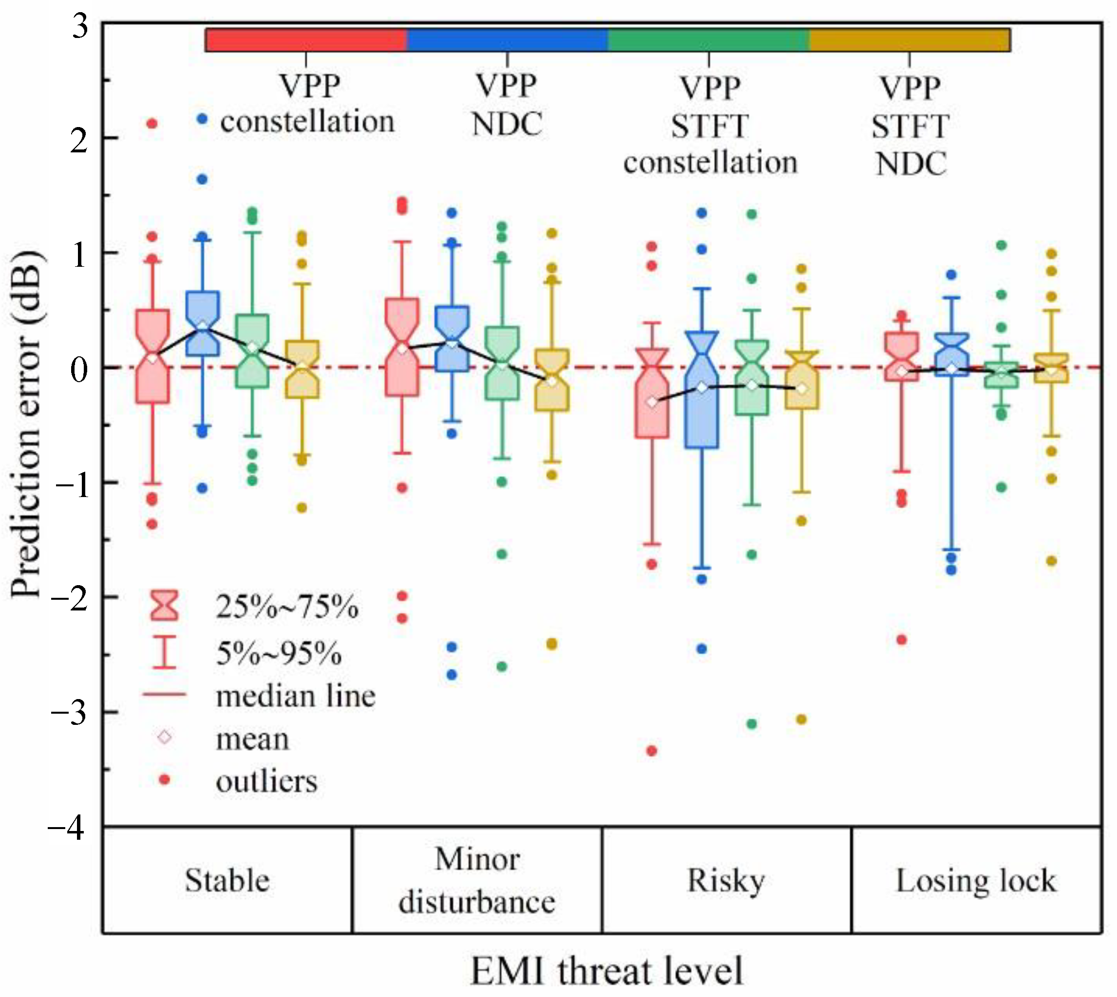
6.3. Prediction Performance

For the above network with four structures, the prediction accuracy of four threat levels is analyzed. The prediction error is set to be different between the actual predicted value ${\widehat{u}}_i$ and the target value $u_i$. Figure 9 shows the boxplot of prediction error under different EMI threat levels, which is used to compare the distribution interval and dispersion degree of the prediction error. The interval of 25~75% shows 50% of the error distribution, indicating the concentration of the error distribution. Similarly, the range of 5~95% shows 90% of the error distribution, indicating the main distribution range of prediction error.

From the perspective of different EMI threat levels, the error distribution of the lose lock level is the most concentrated and the prediction accuracy is the highest. 50% of the error is distributed in [−0.2 dB, 0.3 dB] and 90% in [−1.6 dB, 0.6 dB] with less deviation compared to the other three cases. The distribution of errors in the risky level is more dispersed with relatively large deviation values, more than 3 dB. The double-input network with the inputs of VPP and constellation diagram has larger outliers, and the 90% error distribution of the three-channel network with the inputs of VPP, constellation diagram, and STFT is relatively wide. In contrast, the error distribution of the network using NDC is more concentrated, of which the mean and median are closer to 0, and 5~95% of the error is concentrated in [−1 dB, 1 dB]. Among them, the three-input network with NDC has the best prediction performance.

6.4. Prediction Performance

In order to compare the performance of the proposed MIMT-CNN and the existing state-of-the-art model under multi-task networks, we replace the part of feature fusion processing in Figure 6 with four classical CNN structures (AlexNet, GoogLetNet, VGG, ResNet), and use the same data set to train the model. The performance of MIMT-CNN and classical CNN structures on the training set is shown in Figure 10. Although the threat prediction RMSE of MIMT-CNN is slightly worse than that of AlexNet, MIMT-CNN has the highest classification accuracy of EMI among the classical models. On the whole, MIMT-CNN achieves the best balance between classification and prediction performance.

Some typical areas of interference identification and threat prediction models are listed in

Table 5. Comparison of model performance.

Reference	Accuracy	RMSE	Algorithm	Application Scenario
Interference identification and threat assessment (this work)-Multi-task
Proposed Model	95.45%	0.49	CNN
Interference identification- Single-task
[34]	86.97%	-	CNN	Cognitive radio equipment
[35]	89%	-	U-Net	Radar receiver
[36]	92.7%	-	FCN	Engine digital controllers
[37]	96.53%	-	ResNet	High voltage power plants
Threat assessment- Single-task
[38]	-	0.975	DNN	Financial loss
[39]	-	0.518	CNN-LSTM	Water quality risk
[10]	-	0.3882	CNN	Data link under EMI
[40]	-	0.231	DNN	Flood risk

. It can be concluded that CNN is a commonly used model in the field of interference identification and classification evaluation and has good results under single-task application. In the case of multi-task, the accuracy and RMSE of MIMT-CNN reaches a good level.

7. Conclusions

Given the vulnerability and insufficient awareness of the UAV data link to the EMI threat, this paper proposes a multi-task CNN with multi-input (MIMT-CNN) to realize the EMI signal identification and risk assessment of the UAV data link. Based on the multi-task learning and multi-information fusion, the network extracts EMI features by inputting visualized performance parameters, STFT spectrogram and normalized density constellation, and then fuses these features by using the parallel structures optimized by the Bayesian algorithm. By extending the traditional serial structure, the network can extract more complex EMI signal features and make full use of the correlation information among the input features through multi-task outputs. Compared with learning each task separately, it can reduce the time cost, calculation cost, and storage cost of the network.

By changing the categories of the input images of the MIMT-CNN for training and testing, it is found that the visualized performance parameters are the basis of model validity, while the STFT spectrogram or constellation diagram can improve model accuracy. Among them, the network with the best classification and regression performance can be obtained by inputting the visualized performance parameters, STFT spectrogram, and normalized density constellation, but the time cost will increase with the network complexity.

The cognition of EMI types and threat levels contributes to the self-awareness of the data link. Furthermore, it can be combined with interference suppression technology to achieve a fast and accurate confrontation strategy on the UAV platform, so that the UAV will obtain the ability of self-healing.

References

- Mehta, P.; Gupta, R.; Tanwar, S. Blockchain envisioned UAV networks: Challenges, solutions, and comparisons. Comput. Commun. 2020, 151, 518–538. [Google Scholar] [CrossRef]
- Ch, R.; Srivastava, G.; Reddy Gadekallu, T. Security and privacy of UAV data using blockchain technology. J. Inf. Secur. Appl. 2020, 55, 102670. [Google Scholar] [CrossRef]
- Le Cun, Y.; Bengio, Y.; Hinton, G. Deep learning. Nature 2015, 521, 436–444. [Google Scholar] [CrossRef] [PubMed]
- Wu, C.; Kim, H.; Penugonda, S.; Fan, J. Analysis and modeling of the common-mode conducted EMI from a wireless power transfer system for mobile applications. IEEE Trans. Electromagn. Compat. 2021, 63, 2143–2150. [Google Scholar] [CrossRef]
- Han, J.H.; Ju, S.H.; Kang, N.W.; Lee, W.S.; Choi, J.S. Wideband coupling modeling analysis by arbitrarily incoming source fields based on the electromagnetic topology technique. IEEE Trans. Microw. Theory Tech. 2019, 67, 28–37. [Google Scholar] [CrossRef]
- Houret, T.; Besnier, P.; Vauchamp, S.; Pouliguen, P. Probability of failure using the kriging-controlled stratification method and statistical inference. In Proceedings of the 2020 International Symposium on Electromagnetic Compatibility, Rome, Italy, 23–25 September 2020. [Google Scholar]
- Genender, E.; Garbe, H.; Sabath, F. Probabilistic risk analysis technique of intentional electromagnetic interference at system level. IEEE Trans. Electromagn. Compat. 2014, 56, 200–207. [Google Scholar] [CrossRef]
- Zhang, D.X.; Zhao, M.; Cheng, E.W.; Chen, Y.Z. GPR-based EMI prediction for UAV’s dynamic datalink. IEEE Trans. Electromagn. Compat. 2021, 63, 19–29. [Google Scholar] [CrossRef]
- Devaraj, L.; Ruddle, A.R.; Duffy, A.P. EMI risk estimation for system-level functions using probabilistic graphical models. In Proceedings of 2021 IEEE International Joint EMC/SI/PI and EMC Europe Symposium, Raleigh, NC, USA, 24 July–13 August 2021; IEEE: Piscataway, NJ, USA, 2021; pp. 851–856. [Google Scholar]
- Xu, T.; Wang, Y.M.; Zhang, D.X.; Zhao, M.; Chen, Y.Z. Prediction on EMS of UAV’s data link based on SSA-optimized dual-channel CNN. IEEE Trans. Electromagn. Compat. 2022, 64, 1346–1356. [Google Scholar] [CrossRef]
- Zhou, H.; Jiao, L.; Zheng, S.; Yang, L.; Shen, W.; Yang, X. Generative adversarial network-based electromagnetic signal classification: A semi-supervised learning framework. China Commun. 2020, 17, 157–169. [Google Scholar] [CrossRef]
- Jin, H.; Gu, Z.M.; Tao, T.M.; Li, E. Hierarchical attention-based machine learning model for radiation prediction of WB-BGA package. IEEE Trans. Electromagn. Compat. 2021, 63, 1972–1980. [Google Scholar] [CrossRef]
- Shu, Y.; Wei, X.; Fan, J.; Yang, R.; Yang, Y. An equivalent dipole model hybrid with artificial neural network for electromagnetic interference prediction. IEEE Trans. Microw. Theory Tech. 2019, 67, 1790–1797. [Google Scholar] [CrossRef]
- Yuan, S.; Lin, P.; Chang, C.; Dong, J.; Su, C. Classification of an embedded system instruction EMI using a deep convolutional neural network. In Proceedings of 2019 Joint International Symposium on Electromagnetic Compatibility and Asia-Pacific International Symposium on Electromagnetic Compatibility, Sapporo, Japan, 3–7 June 2019; IEEE: Piscataway, NJ, USA, 2019; pp. 338–341. [Google Scholar]
- Zhang, H.; Yuan, L.; Wu, G.; Zhou, F.; Wu, Q. Automatic modulation classification using involution enabled residual networks. IEEE Wirel. Commun. Lett. 2021, 10, 2417–2420. [Google Scholar] [CrossRef]
- Sun, G. RF transmitter identification using combined siamese networks. IEEE Trans. Instrum. Meas. 2021, 71, 8000813. [Google Scholar] [CrossRef]
- Zhang, Y.; Yang, Q. A survey on multi-task learning. IEEE Trans. Knowl. Data Eng. 2022, 34, 5586–5609. [Google Scholar] [CrossRef]
- Maddikunta, P.K.R. Unmanned aerial vehicles in smart agriculture: Applications, requirements, and challenges. IEEE Sens. J. 2021, 21, 17608–17619. [Google Scholar] [CrossRef]
- Hamdalla, M.Z.; Roacho-Valles, J.M.; Caruso, A.N.; Hassan, A.M. Electromagnetic Compatibility Analysis of Quadcopter UAVs Using the Equivalent Circuit Approach. IEEE Open J. Antennas Propag. 2022, 3, 1090–1101. [Google Scholar] [CrossRef]
- Peng, S.; Sun, S.; Yao, Y.D. A survey of modulation classification using deep learning: Signal representation and data preprocessing. IEEE Trans. Neural Netw. Learn. Syst. 2021, 33, 7020–7038. [Google Scholar] [CrossRef]
- Zhang, W.T.; Cui, D.; Lou, S.T. Training images generation for CNN based automatic modulation classification. IEEE Access 2021, 9, 62916–62925. [Google Scholar] [CrossRef]
- Tang, B.; Tu, Y.; Zhang, Z.; Lin, Y. Digital signal modulation classification with data augmentation using generative adversarial nets in cognitive radio networks. IEEE Access 2018, 6, 15713–15722. [Google Scholar] [CrossRef]
- Olshausen, B.A.; Field, D.J. Natural image statistics and efficient coding. Netw. Comput. Neural Syst. 1996, 7, 333–339. [Google Scholar] [CrossRef]
- Jacek, T.; Kwolek, B. Multi-channels CNN temporal features for depth-based action recognition. In Proceedings of the 12th International Conference on Machine Vision, Amsterdam, The Netherlands, 16–18 November 2020. [Google Scholar]
- Wang, G.; Giannakis, G.B.; Chen, J. Learning relu networks on linearly separable data: Algorithm, optimality, and generalization. IEEE Trans. Signal Process. 2019, 67, 2357–2370. [Google Scholar] [CrossRef] [Green Version]
- Hareth, S.; Mostafa, H.; Shehata, K.A. Low power CNN hardware FPGA implementation. In Proceedings of the 31st IEEE International Conference on Microelectronics, Cairo, Egypt, 15–18 December 2019; IEEE: Piscataway, NJ, USA, 2019. [Google Scholar]
- Szegedy, C. Going deeper with convolutions. In Proceedings of IEEE Conference CVPR, Boston, MA, USA, 8–10 July 2015; IEEE: Piscataway, NJ, USA, 2015; pp. 1–9. [Google Scholar]
- Awais, M.; Bin Iqbal, M.T.; Bae, S.H. Revisiting internal covariate shift for batch normalization. IEEE Trans. Neural Netw. Learn. Syst. 2021, 32, 5082–5092. [Google Scholar] [CrossRef] [PubMed]
- Lin, T.Y.; Goyal, P.; Girshick, R.; He, K.; Dollár, P. Focal loss for dense object detection. IEEE Trans. Pattern Anal. Mach. Intell. 2020, 42, 318–327. [Google Scholar] [CrossRef] [PubMed] [Green Version]
- Shahriari, B.; Swersky, K.; Wang, Z.; Adams, R.P.; Freitas, N.D. Taking the human out of the loop: A review of bayesian optimization. Proc. IEEE 2016, 104, 148–175. [Google Scholar] [CrossRef] [Green Version]
- Snoek, J.; Larochelle, H.; Adams, R.P. Practical bayesian optimization of machine learning algorithms. Adv. Neural Inf. Process. Syst. 2012, 25, 1467–5463. [Google Scholar]
- Dolatsara, M.A.; Hejase, J.A.; Becker, W.D.; Kim, J.; Lim, S.K.; Swaminathan, M. Worst-case eye analysis of high-speed channels based on bayesian optimization. IEEE Trans. Electromagn. Compat. 2021, 63, 246–258. [Google Scholar] [CrossRef]
- Ma, Y.; Guo, R.; Li, M.; Yang, F.; Xu, S.; Abubakar, A. Supervised descent method for 2D magnetotelluric inversion using Adam optimization. In Proceedings of 2019 International Applied Computational Electromagnetics Society Symposium, Nanjing, China, 8–11 August 2019; IEEE: Piscataway, NJ, USA, 2019. [Google Scholar]
- Mossad, O.S.; El Nainay, M.; Torki, M. Deep convolutional neural network with multi-task learning scheme for modulations recognition. In Proceedings of the 2019 15th International Wireless Communications & Mobile Computing Conference (IWCMC), Tangier, Morocco, 24–28 June 2019; IEEE: Piscataway, NJ, USA, 2019. [Google Scholar]
- Wang, J.; Wang, H.; Sun, Z. Research on the effectiveness of deep convolutional neural network for electromagnetic interference identification based on I/Q data. Atmosphere 2022, 13, 1785. [Google Scholar] [CrossRef]
- Wei, M.; Chen, K.; Li, S.; Cao, J.; Ali, A. An intelligent method based on time-frequency analysis and deep learning semantic segmentation for investigating the electromagnetic pulse features of engine digital controllers. IEEE Trans. Electromagn. Compat. 2023, 65, 257–270. [Google Scholar] [CrossRef]
- Mitiche, I.; Jenkins, M.D.; Boreham, P.; Nesbitt, A.; Morison, G.H. An expert system for EMI data classification based on complex Bispectrum representation and deep learning methods. Expert Syst. Appl. 2021, 171, 114568. [Google Scholar] [CrossRef]
- Kim, J.M.; Bae, J.; Son, S.; Son, K.; Yum, S.G. Development of model to predict natural disaster-induced financial losses for construction projects using deep learning techniques. Sustainability 2021, 13, 5304. [Google Scholar] [CrossRef]
- Barzegar, R.; Aalami, M.T.; Adamowski, J. Short-term water quality variable prediction using a hybrid CNN-LSTM deep learning model. Stoch. Environ. Res. Risk Assess. 2020, 34, 415–433. [Google Scholar] [CrossRef]
- Pham, B.T. Flood risk assessment using deep learning integrated with multi-criteria decision analysis. Knowl.-Based Syst. 2021, 219, 106899. [Google Scholar] [CrossRef]