Article

Prediction Method for Sugarcane Syrup Brix Based on Improved Support Vector Regression

College of Mechanical Engineering, Guangxi University, 100 Daxue East Road, Nanning 530004, China
*
Author to whom correspondence should be addressed.
Electronics 2023, 12(7), 1535; https://doi.org/10.3390/electronics12071535
Submission received: 8 February 2023 / Revised: 16 March 2023 / Accepted: 20 March 2023 / Published: 24 March 2023
(This article belongs to the Special Issue Application of Machine Learning and Intelligent Systems)

Abstract

:
The brix of syrup is an important parameter in sugar production. To accurately measure syrup brix, a novel measurement method based on support vector regression (SVR) is presented. With the resonant frequency and quality factor as inputs and syrup brix as the output, a mathematical model of the relationship between the resonant frequency, quality factor, and syrup brix is established. Simultaneously, the particle swarm optimization (PSO) algorithm is used to optimize the penalty coefficient and radial basis kernel function of SVR to improve the performance of the model. The calculation model is trained and tested using the collected experimental data. The results show that the mean absolute error, mean absolute percentage error, and root mean square error of the syrup brix calculation model based on the improved SVR model can reach 0.74 °Bx, 2.24%, and 0.90 °Bx, respectively, while the determination coefficient can reach 0.9985. The simulation of the online measurement of syrup brix in the actual production process proves the excellent prediction performance of the syrup brix calculation model based on the improved PSO–SVR model, which can thus be used to predict the syrup brix.

1. Introduction

1.1. Background

The clarification of cane juice and the crystallization of boiled sugar are important processes in sugar production. Both clarification and crystallization affect the quality of sugar and its economic benefit to sugar factories. The brix of syrup is an important monitoring parameter in these two processes. The rapid and accurate measurement of syrup brix is essential to realize the automatic control of the sugar manufacturing process and improve product quality [1]. The syrup brix is the percentage by mass of soluble solids (the main component is sugar) in the syrup mixture, and it is expressed as η in °Bx.

1.2. Existing Syrup Brix Measurement Methods Research

At present, several measurement methods have been proposed, among which the conductivity method, refractive index method, density method, and microwave method are the most common. The syrup is a mixture containing electrolytes that ionize positive and negative ions in water and thus have electrical conductivity, so the syrup brix can be calculated by measuring the electrical conductivity in the syrup solution. Marzougui et al. [2] developed a method in which gamma-irradiated solid table sugar was investigated for dosimetry, and the absorbed dose was estimated by measuring the conductivity of aqueous solutions of dissolved irradiated solid sugar. The results showed that the electrical conductivity of the solution increases linearly with the dose absorbed. However, in actual production, the purity of the cane juice that is squeezed from sugarcane of different varieties and different origins varies, and the composition and quantity of the electrolytes contained also vary. Therefore, the conductivity of the syrup mixture fluctuates within a certain range during the production process, that is, there is a large error in the brix value when measured by the conductivity. In contrast, it is more accurate to use the refractive index to measure the syrup brix. Li et al. [3] developed a refraction laser–CCD molasses malleability sensor with a high stability laser light source and a high-performance CCD charge-coupled device, which can automatically detect the syrup brix and add temperature compensation with a measurement error of 0.3%. Dongare et al. [4] presented a mathematical model of the optical geometry of a prismatic refractometer for syrup brix measurement, and the simulation and experimental results showed a good correlation. However, due to the poor penetration of the refractometer, a surface layer of 0.1 μm thickness is sufficient to greatly change the intensity of the light transmission. Therefore, when a small amount of dirt is generated on the lens and not cleaned in time, the refractive index will change significantly, which will seriously affect the accurate measurement of the instrument. The density method uses a pre-developed mathematical model of syrup brix and density, including comparison tables, empirical data fitting formulas, etc., in order to obtain the syrup brix measurement by looking up the table or substituting it into the calculation formula after measuring the density of syrup [5]. Nunak et al. [6] developed an instrument to measure the concentration of sugar solutions using a relative density. The results showed that the instrument can accurately analyze the concentration. Huang et al. [7] designed an online automatic detection system for syrup brix based on the density method and PLC technology, and added linear programming correction and temperature compensation, which can obtain a more accurate brix value. Although the density method has a simple measurement principle and low cost, the measurement range is narrow, the structure of the measuring device is complicated, and the measurement accuracy depends on the accuracy of the processing and assembly of the measuring device, which easily leads to large measurement errors and poor stability. Microwave technology can be used as an alternative method for food analysis [8]. The microwave method has the advantages of a simple mechanical structure, no harm to the sample, and high measurement accuracy. In addition, due to the strong penetration of the microwave, the micro dirt generated in the measurement site has little impact on the measurement, so it has high stability. Hosseini et al. [9] proposed a new technique that enables a microwave resonator to perform a volume fraction analysis of complex dynamically changing liquids, while maintaining the original characteristics of the microwave resonator sensor. Multiple simulations and experimental results validated the ability of this technique to monitor ethanol, water, and sugar concentrations in real time during fermentation. However, this method cannot yet be used in the sugar production process. Liu et al. [
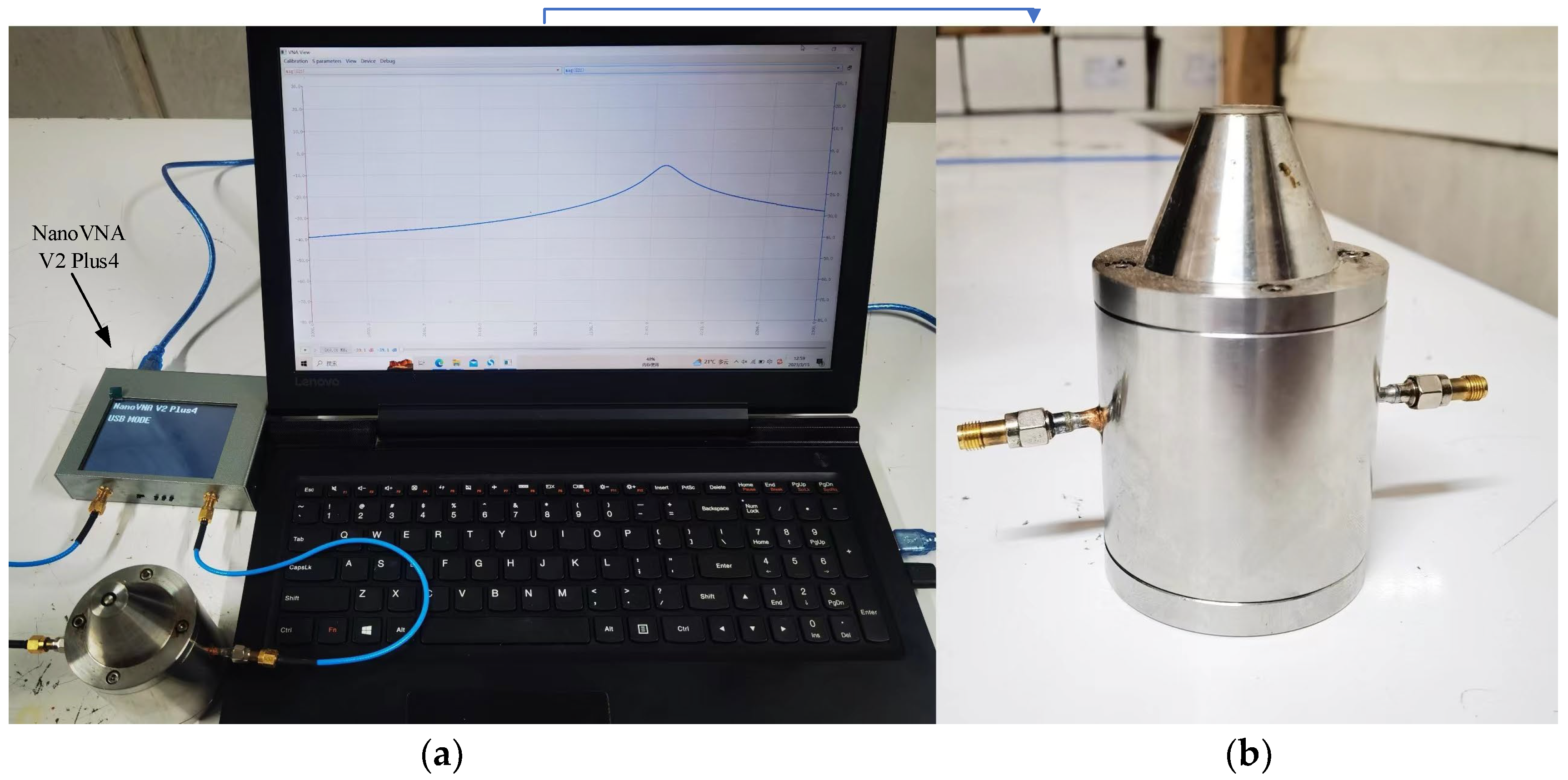
10] designed a microwave coaxial resonator sensor to characterize the syrup brix by measuring the resonant frequency and quality factor of the syrup, which exhibited an excellent performance when measuring brix, with an accuracy equivalent to that of the brix meter produced by Germany’s proMtec in the actual sugar manufacturing process [11]. However, this method did not investigate the model used to calculate the syrup brix.
As can be seen, the current measurement of syrup brix is mainly focused on finding more suitable measurement methods, and little research has been conducted in order to improve the accuracy of the brix calculation model. On this basis, this paper adopts the microwave method to measure the syrup brix, using the microwave coaxial resonant cavity in [10] as the measurement sensor, and conducts further research to improve the accuracy of the sugar brix calculation model.
When the microwave method is used for measurement, the syrup brix is usually calculated by the model based on the mixed dielectric law. The syrup is a mixed solution; hence, the complex permittivity of each component is different. According to the mixed dielectric law, when the proportion of each component is different, their complex permittivity also varies [12]. According to this feature, a theoretical calculation model can be established to derive the brix from the resonant frequency and quality factor. However, measurement errors are caused by the measurement hardware and the approximate processing of the theoretical calculation model based on the microwave perturbation method and mixed dielectric law. The accumulation of these errors will lead to relatively large measurement errors. A stable measurement system will reduce the fluctuations in the measurement errors of the resonant frequency and quality factor. Therefore, the negative impact of these errors on the measurement accuracy can be reduced or eliminated by directly establishing the numerical values of the resonant frequency, quality factor, and the syrup brix. Regression fitting is a method that is widely used to establish measurement models in measurement technology. Using the regression fitting method to establish the regression equation of the relationship between the resonant frequency, quality factor, and brix, a calculation model can be developed based on multiple regression to reduce the negative impact of the above errors. Multiple regression analysis describes the mathematical relationships between the overall trends in the resonance parameters and syrup brix. However, these cannot be accurately predicted when the data significantly deviate from the fitting curve.
The support vector machine (SVM) is a new machine learning algorithm that was proposed by Vapnik et al. based on the statistical learning theory, which can be used for the classification of small samples [13]. The SVM performs the nonlinear mapping of the input vector from the low-dimensional to the high-dimensional feature space. It adopts the principle of structural risk minimization to improve the generalization ability of the model and avoid the “dimensional disaster”. For regression fitting, Vapnik et al. [14] proposed the insensitive loss function τ based on the SVM classification to enable the construction of a support vector regression (SVR) algorithm with superior performance. Compared with other algorithms, such as random forest (RF), radial basis function (RBF), and artificial neural network (ANN), SVR is more suitable for complex and nonlinear regression problems when they are based on statistical supervised learning theory and structural risk minimization. It has a sound theoretical foundation, strong fitting ability, strong generalization ability, and strong robustness [15]. SVR has been applied to solve many problems. Castro-Neto et al. [16] presented the application of a supervised statistical learning technique called Online-SVR, which was used to predict the short-term traffic flow; the results showed that its performance was better than other models. Liang et al. [17] proposed a fuzzy multilevel algorithm based on PSO to optimize SVR in order to realize the real-time dynamic evaluation of drilling risk; the results showed that the accuracy of the PSO–SVR model can reach 99.99%, which is obviously better than that of the multilayer perceptron neural network model. Quan et al. [18] established an SVR model by using the measured water temperature data in a reservoir for many years, and the genetic algorithm was introduced to optimize the parameters; the results showed that this model could predict the vertical water temperature and water temperature structure in the reservoir area well. Benkedjouh et al. [19] presented a method that was based on nonlinear feature reduction and SVR in order to assess the condition of tools and predict their life; the results showed that the proposed method was suitable for assessing the wear evolution of the cutting tools and predicting their remaining useful life. Paniagua-Tineo et al. [20] presented a method based on SVR for daily maximum temperature prediction, and different meteorological variables were obtained, including temperature, precipitation, relative humidity, air pressure, the synoptic situation of the day, and the monthly cycle. By using this pool of prediction variables, it was shown that the SVR could accurately predict the maximum temperature 24 h later. Li et al. [21] developed an improved gray wolf optimization algorithm to optimize the SVR in order to estimate knee joint extension force accurately and timely; the indexes showed that this model provided the best performance and was better than other models. In summary, it can be seen that SVR can be used for syrup brix prediction.
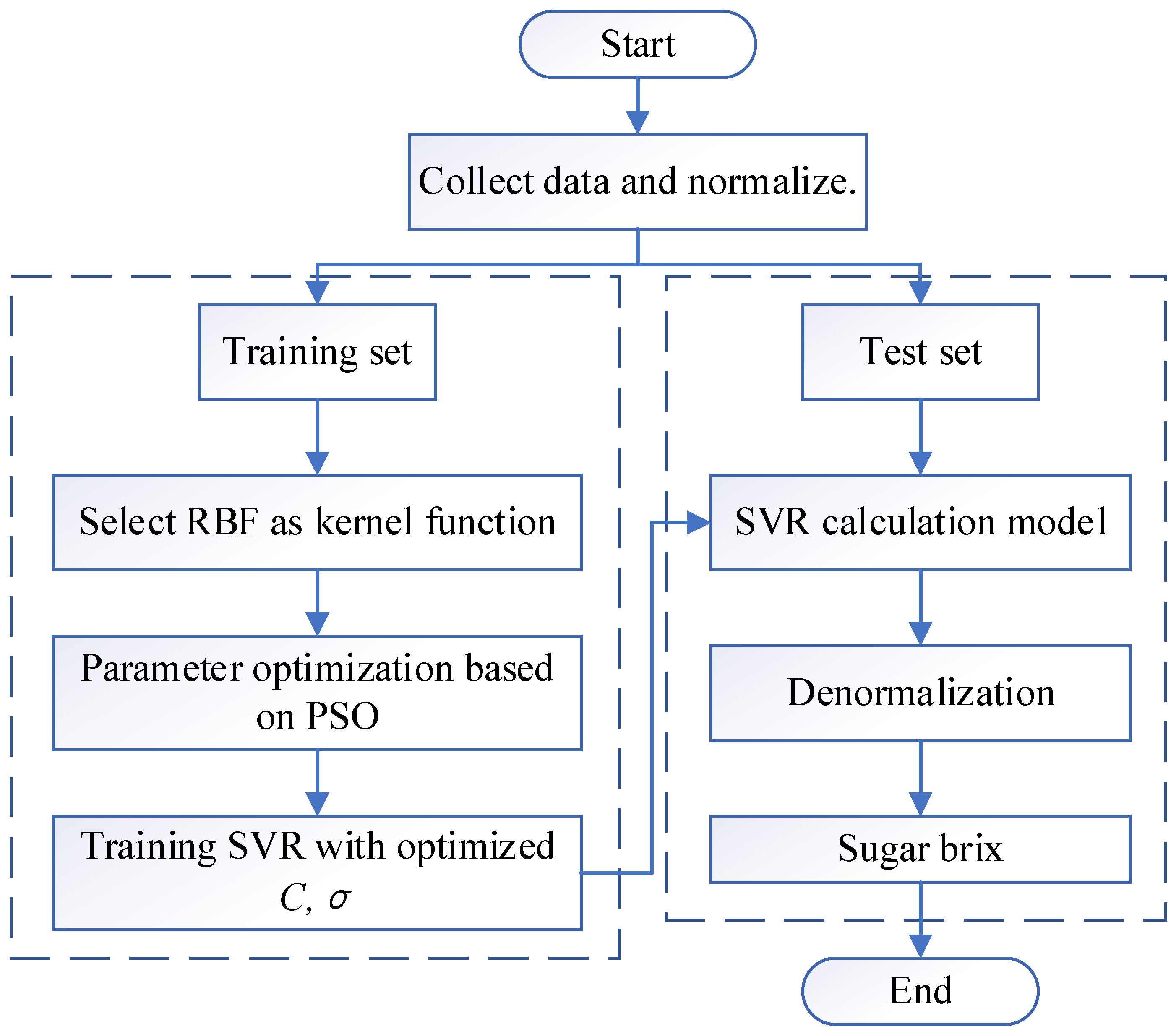
To improve the accuracy of the syrup brix calculation model, this paper studies an SVR-based syrup brix calculation model, optimizes the SVR using improved particle swarm optimization (PSO), and establishes a one-to-one mapping relationship between the resonant parameters and syrup brix. Compared with other calculation models, the PSO–SVR model could obtain the best performance using different evaluation indexes.

1.3. Contributions

The main contributions of this paper are as follows:
  • A new SVR-based syrup brix calculation model is introduced, and the improved PSO is used to optimize the key SVR parameters. The adaptive PSO has multiple inertia weights, which can balance the global and local search abilities.
  • The first application of the proposed PSO–SVR model in syrup brix calculation.
  • It is the first time that a method combining the microwave method with the PSO–SVR calculation model is used to predict the syrup brix.
The rest of the paper is structured as follows: In Section 2, we introduce the data collection, experimental setup, the theory of the SVR and PSO, and the improvement of the PSO; then, we establish the PSO–SVR model and the other two traditional models, finally introducing the evaluation indexes. In Section 3, we show the results of the PSO–SVR model and the comparison with other models; then, we simulate the online measurement of the syrup. In Section 4, we present our conclusions and avenues for future research.

2. Materials and Methods

2.1. Data Collection

A number of methyl syrups that had not been completely boiled were obtained from a sugar factory in Nanning, Guangxi, China. A total of 200 samples of syrup with a density of 10–90 °Bx were prepared and placed in volumetric cups. The brix value within this range was random. The brix range was set as 10–90 °Bx because the syrup brix was greater than 10°Bx in the sugar production process. The maximum brix of the original syrup was 90 °Bx because of the limited experimental conditions. In addition, samples of standard syrups with brix values of 60, 65, 70, 75, 80, 85, and 90 °Bx (60–90 °Bx is the required range for the sugar crystallization process) were prepared to simulate the online brix measurement of the actual sugar crystallization process. The brix of the syrup samples was measured using a fully automatic refractometer (DigiPol-R600, Shanghai Jiahang Instrument Company), and the measured values were taken as the standard values. The refractometer had a measurement range of 0–100 °Bx and a measurement accuracy of 0.01 °Bx.
The steps in the experimental data collection are as follows:
Step 1: Pour the appropriate amount of syrup into a volumetric cup. Use a rubber tip dropper to draw distilled water and inject it into the cup. Mix the syrup and water slowly and evenly using a glass rod.
Step 2: Let the syrup stand for 10 min to allow the bubbles to rise to the surface. Use the dropper to draw a small amount of syrup from the cup and place it in the measuring area of the automatic refractometer to record the measured brix value.
Step 3: Repeat Steps 1 and 2 until 200 standard syrup samples of 10–90 °Bx and seven standard syrup samples of 60, 65, 70, 75, 80, 85, and 90 °Bx are prepared.
Step 4: Immerse the open end of the developed coaxial resonator into the syrup sample, maintain an immersion depth of 1 cm, and record the measured resonant frequency and quality factor.
Step 5: Repeat Step 4 until all samples are collected.
If a group of data collected significantly deviates from the actual situation, it shall be discarded, and the measurement shall be conducted again after checking the equipment.

2.2. Experimental Setup

The experimental setup is shown in Figure 1. In this experiment, a self-designed microwave coaxial resonator was used as the measurement sensor. The resonator sensor was connected to the NanoVNA V2 Plus4 vector network analyzer by two coaxial cables (A-info SM-SM-SFD147A, DC-18GHz). The analyzer was developed by HCXQS in collaboration with OwOComm. The frequency of the analyzer ranged from 50 kHz to 4.4 GHz, the frequency resolution was 1 Hz, and the power resolution was 0.01 dB. The analyzer was directly connected to a personal computer by a LAN cable. The data were displayed on the NanoVNA-QT and collected using MATLAB. In the test, the analyzer was operated in the network analyzer mode at a frequency of 2.0–2.45 GHz with 2000 sampling points. The calibration method known as SOLT(T/R) was adopted, in which calibration was performed at the port 1 and port 2 connectors. During the test, the open end of the sensor was completely immersed in the syrup. The working principle of the experimental platform is shown in Figure 2.
All experiments were conducted at room temperature (25 ± 1 °C). Special attention was paid to prevent bubbles from forming in the liquid and to ensure that the volume of each liquid sample and the depth of the sensor immersed in the liquid were the same.

2.3. Construction of Syrup Brix Calculation Model Based on SVR

2.3.1. SVR

The basic idea of SVR is to determine the optimal hyperplane in order to minimize the total deviation of all sample points from the hyperplane [22]. For the training sample, set D = { ( x i , y i ) , i = 1 , 2 , , l } ; x i ( x i R d ) is the input vector, x i = [ x i 1 , x i 2 , , x i d ] T , y i R is the corresponding output value, and its regression function is as follows:
f ( x ) = w ϕ ( x ) + b
where ϕ ( x ) is the nonlinear mapping function, w is the coefficient vector, and b is the threshold.
The τ linear insensitive loss function is defined by the following formula:
L ( f ( x ) , y , τ ) = { 0 , | y f ( x ) | τ | y f ( x ) | τ , | y f ( x ) | > τ
where y is the true value corresponding to f ( x ) .
If the error between f ( x ) and y is not greater than τ , then the loss is zero. However, if the error between f ( x ) and y exceeds τ , then a fitting error occurs. Therefore, the relaxation factors ξ i and ξ i * were introduced. The objective function and constraints of SVR are as follows:
{ min 1 2 | | w | | 2 + C i = 1 l ( ξ i + ξ i * ) s .   t .   { y i f ( x i ) τ + ξ i , i = 1 , 2 , , l f ( x i ) y i τ + ξ i * , i = 1 , 2 , , l ξ i , ξ i * 0
where C is the penalty coefficient. The greater the C, the greater the penalty for the sample whose training error exceeds τ . The τ limits the error of the regression function; hence, the lower its value, the smaller the error of the regression function.
According to quadratic programming and the kernel function problem, the following regression functions can be obtained.
f ( x ) = i = 1 l ( α i α i * ) K ( x i , x ) + b *
where the sample x i corresponding to the nonzero coefficient ( α i α i * ) is the support vector, Κ ( x i , x j ) is the kernel function Κ ( x i , x j ) = ϕ ( x i ) · ϕ ( x j ) , and b * is the optimized threshold.
Common kernel functions include the sigmoid kernel function, radial basis function (RBF), and polynomial kernel function [23]. Compared with the other kernel functions, RBF contains only one parameter σ , which is easily optimized in the subsequent model. Therefore, RBF was selected as the kernel function of SVR in this study.

2.3.2. SVR Parameter Optimization

The penalty coefficient C and RBF parameter σ in SVR have a significant impact on the SVR performance. However, their values are unknown. Thus, these two parameters must be optimized to improve the performance of the model.
PSO is a swarm intelligent optimization algorithm that is based on the foraging behavior of birds [24]; using the overall cooperation ability among birds allows the group to achieve the optimal [25]. It has the characteristics of fast convergence and easy realization, and is widely used in problems such as multi-objective optimization [26], function optimization [27], and feature selection [28]. At the same time, the PSO algorithm is simpler compared with the rules of the genetic algorithm [29]. Therefore, in this article, the PSO is used to optimize the above two parameters.
In the PSO, each particle is regarded as a point in the D dimension space, which represents a solution to the optimization problem. Suppose the position of particle i is X i = ( X i 1 , X i 2 , , X i D ) , V i = ( V i 1 , V i 2 , , V i D ) is its current speed, P i = ( P i 1 , P i 2 , , P i D ) is the individual extreme value, and P g = ( P g 1 , P g 2 , , P g D ) is the population extreme value.
In the iteration process, the position and velocity of the particle are updated by the following formulas:
V i d k + 1 = ω V i d k + c 1 r 1 ( P i d k X i d k ) + c 2 r 2 ( P g d k X i d k )
X i d k + 1 = X i d k + V i d k + 1
where N is the number of particles; d = 1 , 2 , D ; i = 1 , 2 , N ; k is the number of iterations; ω is the inertia weight; c 1 and c 2 are the coefficients of acceleration, and r 1 and r 2 are random numbers between 0 and 1.
The individual and group extreme values are updated by the following formulas:
P i d k + 1 = { X i d k + 1 , f i t n e s s ( X i d k + 1 ) < f i t n e s s ( P i d k ) P i d k , f i t n e s s ( X i d k + 1 ) > f i t n e s s ( P i d k )
P g d k + 1 = min { P 1 d k + 1 , P 2 d k + 1 , , P N d k + 1 }
where f i t n e s s ( · ) is the fitness function.
The inertia weight ω in formula (5) reflects the ability of particles to inherit the velocity of the last iteration, which affects their search range. To balance the global and local search abilities of PSO, this study adopted adaptive PSO with multiple inertia weights to optimize the penalty coefficient C and kernel parameter σ .
Let the inertial weight set be W = { ω 1 , ω 2 , , ω s } , in which each weight performs better within a certain optimization stage. The inertial weights of the five algorithms are as follows: EXPI [30], SUGENO [31], CHAOTIC [32], AIWPSO [33], and SSRDIW2 [34], were selected to form the inertial weight set, which has been proven to have better performance [35].
To evaluate the degree of evolution of the algorithm, the degree of K-step evolution is defined as follows:
r ( k ) = 1 f i t n e s s ( P g d k ) f i t n e s s ( P g d k K + 1 ) + f i t n e s s ( P g d k K + 2 ) + + f i t n e s s ( P g d k ) K
where K is a constant. For any l < k, f i t n e s s ( P g d l ) f i t n e s s ( P g d k ) , it can be seen from formula (9) that r ( k ) [0,1). The larger the r ( k ) , the better the algorithm evolution; otherwise, it becomes worse. When k > 0 and k is a multiple of K, the degree of evolution r ( k ) of the algorithm is calculated. If r ( k ) < t (t is the threshold value), then the inertia weight ω s is randomly selected from the inertia weight set W as the current inertia weight; otherwise, it is retained. Because the above inertia weights were randomly selected, the currently selected inertia weights performed worse than the previous inertia weights. This study reduced the negative impact of this situation by decreasing the number of iteration steps; that is, when r ( k ) < t , K is taken as K/2 (if K is an odd number, it is taken as (K + 1)/2); otherwise, K is the initial value. The improved PSO was used to optimize the penalty coefficient C and kernel parameter σ of SVR. The root mean square error (RMSE) of the syrup brix was taken as the fitness value. The optimization process is shown in Figure 3.

2.3.3. Build Calculation Model

The dimensions and orders of magnitude of the resonance frequency, quality factor, and brix are different. If the model is directly constructed, then the characteristics with a large order of magnitude, such as the resonance frequency, will have a more obvious impact on the model, while those with a small order of magnitude, such as the quality factor, will have a small contribution to the model, leading to a lower prediction accuracy. Therefore, to obtain more accurate results, it is necessary to normalize the feature data to make different features comparable. In general, the data are normalized to the interval [−1, 1] using the Min–Max scaling method. The calculation formula is as follows:
x ¯ i = x i 0.5 ( x max + x min ) 0.5 ( x max x min )
where x i is the original data before normalization; x max and x min are the maximum and minimum values in the original dataset, respectively; and x ¯ i is the normalized original data.
To display the predicted output data as the original brix value, the output data should also be reverse-normalized. The formula is as follows:
y = y max y min 2 y ¯ + y max + y min 2
where y is the brix value after reverse normalization; y max and y min are the maximum and minimum values of all the output values of the model, respectively; and y ¯ is the output value of the model.
The syrup brix calculation model based on the improved PSO–SVR model takes the measured resonant frequency and quality factor as the input variables, and the syrup brix as the output variable. The flowchart of the model is shown in Figure 4.

2.4. Calculation Model Evaluation Index

To evaluate the performance of the syrup brix calculation model, the evaluation criteria must be defined to improve the analysis of the results. Suppose there are n test samples, the actual value of the i-th test sample is x i , the measured value of the corresponding i-th test sample is x ^ i , and the mean value of the test sample is x ¯ = i = 1 n x ^ i / n . The mean absolute error (MAE), mean absolute percentage error (MAPE), RMSE, and determination coefficient ( R 2 ) were selected as the evaluation indexes of the model performance [36]. The calculation formula is shown in Table 1. The smaller the MAE, MAPE, and RMSE, and the closer the R 2 is to 1, the better.

3. Results and Discussion

The partial experimental data collected in Section 2.1. are presented in Table 2. The 200 sets of resonance parameters measured were plotted as scatter plots, and the relationship curves between the resonant frequency (f) and syrup brix ( η ), and between quality factor (Q) and η , are shown in Figure 5. In the 200 groups of measured data with a brix range of 10.25–89.24 °Bx, f almost increases with the increase of η , ranging from 2104.46–2177.50 MHz. There is no linear relationship between Q and η , ranging from 72.22–148.86. Some statistical data of the three resonance parameters can be seen in Table 3.

3.1. Calculation of Syrup Brix Based on PSO–SVR Model

3.1.1. Improved SVR Model Training

The training set consists of 150 groups that were randomly selected from the 200 groups of normalized data, while the test set consists of the remaining 50 groups. Because the sample size is small, the 3:1 ratio is selected to divide the training set and test set, which can not only ensure the training effect, but also verify the measurement effect. The training set was primarily used to build the SVR model and optimize the model parameters. The test set was used to test the established model and verify its performance. The improved PSO was used to optimize the penalty coefficient C and kernel function parameter σ of SVR. Other parameters of SVR were set by default. The RMSE of the brix was selected as the fitness of the algorithm. The parameter settings of the improved PSO algorithm are listed in Table 4.
There are two input variables and one output variable in this model. To balance the convergence of the algorithm, take c 1 = c 2 = 1.5, which is the improved PSO with 300 iterations, other parameters are set based on experience and actual conditions.
The fitness curve of the PSO is shown in Figure 6. In order to compare the performance of the PSO, grid search (GS) was used to optimize SVR. Figure 7 shows the contour map for SVR parameter selection, and the optimized parameter results of these two methods are listed in Table 5. It can be seen from the results that although GS can take less time, the fitness RMSE is significantly greater than the PSO. The fitness RMSE of the PSO is low (0.74 °Bx), indicating its capabilities for strong optimization.
Using the optimized C and σ by PSO, the training set was used for model training in order to build the PSO–SVR model. The training results are shown in Figure 8.

3.1.2. PSO–SVR Model Test

To test the prediction performance of the PSO–SVR model after training, the resonant frequency and quality factor of 50 groups of data in the test set were input into the SVR and PSO–SVR models, respectively. The comparison between the predicted brix values of the model and the real values measured by the refractometer are shown in Figure 9 and Figure 10.
SVR model:
Figure 9. Measurement results of syrup brix based on SVR in the independent test set. (a) Measurement results of brix; (b) Measurement errors of brix.
Electronics 12 01535 g009
PSO–SVR model:
Figure 10. Measurement results of syrup brix based on PSO–SVR in the independent test set. (a) Measurement results of brix; (b) Measurement errors of brix.
Electronics 12 01535 g010
Table 6 shows the evaluation index values of the syrup brix calculation model based on the SVR and PSO–SVR models. To eliminate the errors caused by the algorithm and improve its accuracy, the algorithm was run 10 times. The average values are listed in Table 6. It can be seen that the MAE, MAPE, and RMSE of the modified syrup brix significantly decreased compared with previous values, and that the R 2 is closer to 1. This indicates that the syrup brix values predicted by the PSO–SVR model strongly agree with the brix values measured by the refractometer. Thus, the PSO–SVR model performs well in terms of prediction and generalization.

3.2. Comparison and Analysis of Measurement Results

To verify the performance of the syrup brix calculation model based on PSO–SVR, syrup brix calculation models based on the mixed dielectric law and on multiple regression were introduced for comparison.
A syrup is a mixture that consists of many components. Its complex dielectric constant is not only related to the complex dielectric constant of each component, but also to the proportion of each component. The dielectric constant of the mixture is generally described by the equivalent dielectric constant, which is a macroscopic reflection of the electric field of the mixed medium. The mixed dielectric law characterizes the relationship between the complex permittivity of the mixture and the complex permittivity and content of its components. Its mathematical expression is called the mixed dielectric model. Through theoretical derivation and data fitting, the syrup brix calculation model based on the mixed dielectric law is obtained as follows:
η = 2879 ( 1 f 2291.16 ) + 1029 ( 1 Q 1 186.52 ) + 239.1 25.42 ( 1 f 2291.16 ) 1.159 ( 1 Q 1 186.52 ) + 2.473
The measurement results using this model are shown in Figure 11.
Regression analysis is a statistical analysis method that approximates the relationship between variables. It selects the appropriate mathematical functions when the relationship between the independent variables and dependent variables is unknown, in order to minimize the overall deviation between the curve and the data of the independent variables. The selected functions are called regression equations. The resonant parameters measured by the resonant cavity sensor include two independent variables: the resonance frequency and the quality factor; hence, multiple regressions can be used to fit the relationship between the brix, resonance frequency, and quality factor. The brix of syrup η is fitted with the resonant frequency f and quality factor Q using the binary quadratic polynomial. The calculation model of the syrup brix based on multiple regression can be obtained as follows:
η = 18330 + 17.53 f 24.77 Q 0.004161 f 2 + 0.01106 f Q + 0.005055 Q 2
The measurement results using this model are shown in Figure 12.
By testing the three calculation models with the experimental dataset, the evaluation indicators in Table 7 can be compared.
Table 7 shows that the three error evaluation indicators of the syrup brix calculation model based on the PSO–SVR model are lower than those of the mixed dielectric and multiple regression models. The R 2 is also the closest to 1; hence, it is the best syrup brix calculation model. There are two main causes of the large measurement error in the syrup brix calculation model based on the mixed dielectric law. The first is the error caused by simplification and approximation during the process of establishing the theoretical calculation model; this error is caused by the model itself. The second is the external interference encountered by the microwave signal during measurement, and the accuracy problems that exist in the measurement hardware; these are errors caused by the measurement method. The superposition of these two types of errors eventually leads to large measurement errors. The multiple regression and PSO–SVR models utilize the principle of nonlinear fitting to directly establish the relationship between the resonant frequency, quality factor, and syrup brix from a numerical point of view. They make full use of the information contained in the actual data and significantly reduce the errors caused by the model itself; thus, the measurement error is obviously smaller than that of the mixed dielectric model. In addition, the PSO–SVR model has a stronger numerical mapping ability than the multiple regression model because of the introduction of the kernel function; hence, the measurement effect improves.

3.3. Online Measurement of Simulated Syrup Brix

During sugar production, as the syrup flows into the sugar jar, the syrup is transformed from a Newtonian into a non-Newtonian fluid when the brix reaches the critical value. This changes the viscosity of the brix, which could cause a change in the resonance parameter with the change in the brix. Therefore, to verify the accuracy of the syrup brix calculation model based on the PSO–SVR model when it is used in practical applications, this study built an online platform for measuring syrup brix with fluidity, as shown in Figure 13. The platform consists of a water tank, propeller, motor, lifting platform, and resonant cavity measurement system. The resonant cavity measurement system consists of a resonant cavity, STM32F103 micro controller, microwave signal source, isolator, demodulator, and display unit. The working principle of it is shown in Figure 14. Substances other than syrups (e.g., water tanks and propellers) close to the opening of the resonant cavity can disrupt the electromagnetic field distribution, which affects the measurement accuracy. Therefore, the opening of the resonant cavity must be located at a certain distance from other non-measuring substances. Because the penetration depth of the microwave signal at 2.45 GHz in pure water is approximately 40 mm, while that in a sugar–water mixture is less than that in water [37], the opening of the resonator should be at least 40 mm away from other non-measuring substances. In the flowing state, the distribution of syrup is uniform and consistent with the actual production, so even if the temperature of syrup in the laboratory is different from the actual production (50–70 °C), the influence of temperature on the measurement can be ignored.
The standard syrup samples prepared with brix of 60, 65, 70, 75, 80, 85, and 90 °Bx were poured into the water tank for the experiments. The lifting platform was adjusted to immerse the open-end face of the sensor in the syrup, the motor was started to rotate the propeller and the syrup flowed at a uniform speed under the action of the propeller to simulate the actual sugar production process. To avoid measurement errors caused by uneven syrup, three measurements were made, and their average values were taken.
The evaluation index of the syrup brix online measurement is listed in Table 8.
A comparison of Table 6 and Table 8 shows that although the three error evaluation indexes in Table 8 are slightly larger than those in Table 6, and that the R 2 is slightly smaller than that in Table 6; however, the measurement evaluation indexes in both cases are very close. The MAE is less than 1 °Bx, indicating that the syrup brix calculation model based on the PSO–SVR model can be used for the online measurement of syrup brix in actual situations.

3.4. Discussion

According to the experimental results, it can be proven that the syrup brix measurement model based on the improved PSO–SVR model has a lower level of error and an R 2 that is closer to 1 compared with those based on the mixed dielectric law and multiple regression models. Thus, the performance of the proposed model is significantly better than that of the other two models. Since the training and test sets are randomly assigned during the experiment, this model can still be applied when the dataset is different. By comparing the results before and after SVR optimization, it can be seen that using the PSO algorithm to optimize C and σ can effectively improve the prediction capabilities of the model. Compared with other syrup brix measurement methods, the PSO–SVR calculation model proposed in this paper is helpful when aiming to quickly and accurately measure the syrup brix during the sugar production process; it thus contributes to improving the benefits of sugar factories.
However, several limitations still exist in this study. From the measurement results, it is clear that most models perform poorly at low brix levels, and that the measured value deviates greatly from the true value; even the predicted brix is negative in the mixed dielectric model. Since the input variables of the PSO–SVR model are resonant frequency and quality factor, the model relies on the use of the microwave method to measure the syrup brix. At the same time, the accuracy of the measurement hardware affects the measurement of the resonant frequency and quality factor, so it also affects the performance of this model. Meanwhile, although the performance of this model is excellent, some parameters are set according to experience. In addition, this model may has potential drawbacks; when the data set is large, the algorithm may take more time. SVR may scale poorly as the number of samples increases; when coupled with the evolutionary approach in order to optimize it, in other datasets, this methodology may be very computationally expensive.
Therefore, in future research, in addition to improving the accuracy of the syrup brix measurement sensor, our efforts will be focused on the further optimization of the model’s combination of parameters or on finding a more excellent model; this may lead to an increased measurement accuracy as, for example, combining PSO with GS might reduce the computation time while obtaining a good fitness value. At the same time, it is necessary to improve the accuracy of prediction under low brix levels.

4. Conclusions

In this study, a new model for measuring syrup brix was proposed. The syrup brix calculation model was established by SVR and optimized by PSO. The one-to-one mapping relationship between the resonance frequency, quality factor, and syrup brix was established. Syrup samples were prepared and used for training and testing. The results showed that the MAE, MAPE, and RMSE could reach 0.74 °Bx, 2.24%, and 0.90 °Bx, respectively, while the R 2 could reach 0.9985. The proposed PSO–SVR model is superior to other existing calculation models in its evaluation indexes. It has thus been proven that this model has high levels of accuracy and an excellent prediction performance, which can be used to predict the brix of syrup.

Author Contributions

Conceptualization, S.H. and Y.M.; methodology, S.H.; software, Y.Z.; validation, Y.Z.; formal analysis, Y.M.; resources, Y.M.; data curation, S.H.; writing—original draft preparation, S.H.; writing—review and editing, Y.M.; project administration, Y.M.; funding acquisition, Y.M. All authors have read and agreed to the published version of the manuscript.

Funding

This research was funded by the National Natural Science Foundation of China (No. 61763001). This research was funded by the National Natural Science Foundation of China (No. 12062001). This research was funded by the Natural Science Foundation of Guangxi Province (No. 2021JJA110041).

Data Availability Statement

The data presented in this study are available on request from the corresponding author. The data are not publicly available since future studies are related to current data.

Acknowledgments

The first author would like to express his gratitude to the National Natural Science Foundation of China (Project No. 61763001), National Natural Science Foundation of China (Project No.12062001) and Natural Science Foundation of Guangxi Province (Project No.2021JJA110041) for supporting this research.

Conflicts of Interest

The authors declare no conflict of interest.

References

  1. Yang, J.; Zhang, J. Discussion on automatic control scheme of sugar crystallization section. China Mod. Educ. Equip. 2008, 4, 106–108. [Google Scholar]
  2. Marzougui, K.; Hamzaoui, A.H.; Farah, K.; Nessib, N.B. Electrical conductivity study of gamma-irradiated table sugar for high-dose dosimetry. Radiat. Meas. 2008, 7, 1254–1257. [Google Scholar] [CrossRef]
  3. Li, Z.; Qin, G.; Mo, L. Automatic laser refractive indexing system for syrup concentration. J. South China Univ. Technol. 1998, 3, 110–115. [Google Scholar]
  4. Dongare, M.L.; Buchade, M.N.; Awatade, M.N.; Shaligram, A.D. Mathematical modeling and simulation of refractive index based brix measurement system. Optik 2014, 3, 946–949. [Google Scholar] [CrossRef]
  5. Yang, Z.; Guan, A.; Yin, X. Application of automatic online detection technology of brix in sugar industry. Guangxi Sugar Ind. 2015, 81, 39–43. [Google Scholar]
  6. Nunak, N.; Suesut, T.; Klongratog, B.; Mongkoltalong, P. In Line Osmotic Process Measurement of Concentration of Sugar Solution. In Proceedings of the International Conference of Engineering, Applied Science and Technology (ICEAST 2012), Bangkok, Thailand, 21–24 November 2012. [Google Scholar]
  7. Huang, S.; Qin, J.; Ye, Q.; Qin, H.; Xu, N.; Chen, J. Research on online automatic measuring system of brix in sugar cane factory. Sugarcane Ind. 2018, 4, 29–33. [Google Scholar]
  8. Blakey, R.T.; Morales-Partera, A.M. Microwave dielectric spectroscopy—A versatile methodology for online, non-destructive food analysis, monitoring and process control. Eng. Agric. Environ. Food 2016, 9, 264–273. [Google Scholar] [CrossRef]
  9. Hosseini, N.; Baghelani, M. Selective real-time non-contact multi-variable water-alcohol-sugar concentration analysis during fermentation process using microwave split-ring resonator based sensor. Sens. Actuators A Phys. 2021, 325, 112695. [Google Scholar] [CrossRef]
  10. Liu, H.; Hu, S.; Meng, Y.; Chen, J.; Li, Z.; Li, J.; Zhang, Y. Online measurement of syrup brix with microwave open coaxial resonator sensor. J. Food Eng. 2022, 322, 110975. [Google Scholar] [CrossRef]
  11. Liu, H.; Mai, Y.; Zhou, D. The practice of microwave technology in the final effect hammer measurement of evaporation. Guangxi Sugar Ind. 2015, 1, 16–19. [Google Scholar]
  12. Meng, M.; Meng, X. Effect of temperature and frequency on dielectric model of cement concrete. Bull. Chin. Ceram. 2018, 37, 1758–1764. [Google Scholar]
  13. Cortes, C.; Vapnik, V. Support-Vector Networks. Mach. Learn. 1995, 20, 273–297. [Google Scholar] [CrossRef]
  14. Drucker, H.; Burges, C.J.; Kaufman, L.; Smola, A.; Vapnik, V. Support vector regression machines. Adv. Neural Inf. Process. Syst. 1996, 9. [Google Scholar] [CrossRef]
  15. Zhang, X.; Tang, X.; Zhu, X.; Gao, X.; Chen, X.; Chen, X. A regression-based framework for quantitative assessment of muscle spasticity using combined EMG and inertial data from wearable sensors. Front. Neurosci. 2019, 13, 398. [Google Scholar] [CrossRef] [PubMed] [Green Version]
  16. Castro-Neto, M.; Jeong, Y.; Jeong, M.; Han, L.D. Online-SVR for short-term traffic flow prediction under typical and atypical traffic conditions. Expert Syst. Appl. 2009, 3, 6164–6173. [Google Scholar] [CrossRef]
  17. Liang, H.; Zou, J.; Li, Z.; Khan, M.J.; Lu, Y. Dynamic evaluation of drilling leakage risk based on fuzzy theory and PSO-SVR algorithm. Future Gener. Comput. Syst. 2019, 95, 454–466. [Google Scholar] [CrossRef]
  18. Quan, Q.; Hao, Z.; Xifeng, H.; Jingchun, L. Research on water temperature prediction based on improved support vector regression. Neural Comput. Appl. 2022, 34, 1–10. [Google Scholar] [CrossRef]
  19. Benkedjouh, T.; Medjaher, K.; Zerhouni, N.; Rechak, S. Health assessment and life prediction of cutting tools based on support vector regression. J. Intell. Manuf. 2015, 26, 213–223. [Google Scholar] [CrossRef] [Green Version]
  20. Paniagua-Tineo, A.; Salcedo-Sanz, S.; Casanova-Mateo, C.; Ortiz-García, E.G.; Cony, M.A.; Hernández-Martín, E. Prediction of daily maximum temperature using a support vector regression algorithm. Renew. Energy 2011, 36, 3054–3060. [Google Scholar] [CrossRef]
  21. Li, Z.; Gao, L.; Lu, W.; Wang, D.; Xie, C.; Cao, H. Estimation of Knee Joint Extension Force Using Mechanomyography Based on IGWO-SVR Algorithm. Electronics 2021, 10, 2972. [Google Scholar] [CrossRef]
  22. Yu, L.; Shi, F.; Wang, H.; Hu, F. MATLAB Intelligent Algorithm Analysis of 30 Cases; Beihang University Press: Beijing, China, 2011. [Google Scholar]
  23. Li, L.; Wang, M.; Zhao, H.; Wang, T.; Zhao, R. Displacement prediction of Baishuihe landslide based on CEEMDAN-BA-SVR-Adaboost model. J. Yangtze River Sci. Res. Inst. 2021, 38, 52–59+66. [Google Scholar]
  24. Deng, W. Research and Application of Multi-Model Soft Sensing Modeling Method. Mater Thesis, Jiangnan University, Wuxi, China, 2012. [Google Scholar]
  25. Kennedy, J.; Eberhart, R. Particle swarm optimization. In Proceedings of the ICNN’95-International Conference on Neural Networks, Perth, Australia, 27 November–1 December 1995; Volume 4, pp. 1942–1948. [Google Scholar]
  26. Yildiz, A.R.; Solanki, K.N. Multi-objective optimization of vehicle crashworthiness using a new particle swarm based approach. Int. J. Adv. Manuf. Technol. 2012, 59, 367–376. [Google Scholar] [CrossRef]
  27. Yang, J.; Si, H. Inversion study of fault regional stress field based on PSO-SVR model. Min. Res. Dev. 2022, 42, 173–179. [Google Scholar]
  28. Khan, H.; Nizami, I.F.; Qaisar, S.M.; Waqar, A.; Krichen, M.; Almaktoom, A.T. Analyzing optimal battery sizing in microgrids based on the feature selection and machine learning approaches. Energies 2022, 15, 7865. [Google Scholar] [CrossRef]
  29. Eseye, A.T.; Zhang, J.; Zheng, D. Short-term photovoltaic solar power forecasting using a hybrid Wavelet-PSO-SVM model based on SCADA and Meteorological information. Renew. Energy 2018, 118, 357–367. [Google Scholar] [CrossRef]
  30. Chen, G.; Huang, X.; Jia, J.; Min, Z. Natural Exponential Inertia Weight Strategy in Particle Swarm Optimization. In Proceedings of the World Congress on Intelligent Control & Automation, Dalian, China, 21–23 June 2006. [Google Scholar]
  31. Lei, K.; Qiu, Y.; He, Y. A new adaptive well-chosen inertia weight strategy to automatically harmonize global and local search ability in particle swarm optimization. In Proceedings of the International Symposium on Systems & Control in Aerospace & Astronautics, Harbin, China, 19–21 January 2006. [Google Scholar]
  32. Feng, Y.; Teng, G.; Wang, A.; Yao, Y. Chaotic Inertia Weight in Particle Swarm Optimization. In Proceedings of the International Conference on Innovative Computing, Kumamoto, Japan, 5–7 September 2007. [Google Scholar]
  33. Nickabadi, A.; Ebadzadeh, M.; Safabakhsh, R. A novel particle swarm optimization algorithm with adaptive inertia weight. Appl. Soft Comput. 2011, 11, 3658–3670. [Google Scholar] [CrossRef]
  34. Adewumi, A.O.; Arasomwan, A.M. An improved particle swarm optimiser based on swarm success rate for global optimisation problems. J. Exp. Theor. Artif. Intell. 2014, 28, 441–483. [Google Scholar] [CrossRef]
  35. Yang, B.; Qian, W. Adaptive Particle swarm optimization algorithm with multiple inertia weights. J. Bohai Univ. (Nat. Sci. Ed.) 2021, 42, 41–48+90. [Google Scholar]
  36. Weisberg, S. Applied Linear Regression; John Wiley & Sons: Hoboken, NJ, USA, 2005. [Google Scholar]
  37. Li, Z.; Meng, Z.; Haigh, A.; Wang, P.; Gibson, A. Characterisation of water in honey using a microwave cylindrical cavity resonator sensor. J. Food Eng. 2021, 292, 110373. [Google Scholar] [CrossRef]
Figure 1. Establishment of experimental platform. (a) Experimental setup; (b) Resonant cavity.
Electronics 12 01535 g001
Figure 2. Working principle of experimental platform.
Electronics 12 01535 g002
Figure 3. Flowchart of the improved PSO to optimize the parameters of the SVR model.
Electronics 12 01535 g003
Figure 4. Model of syrup brix measurement based on PSO–SVR.
Electronics 12 01535 g004
Figure 5. Relationship curves between f and η , and between Q and η . (a) f and η ; (b) Q and η .
Electronics 12 01535 g005
Figure 6. Fitness curve (PSO).
Electronics 12 01535 g006
Figure 7. GS–SVR parameter selection diagram (contour map).
Electronics 12 01535 g007
Figure 8. Training results of PSO–SVR model.
Electronics 12 01535 g008
Figure 11. Measurement results of syrup brix based on mixed dielectric model in the independent test set. (a) Measurement results of brix; (b) Measurement errors of brix.
Electronics 12 01535 g011
Figure 12. Measurement results of syrup brix based on multiple regression fitting in the independent test set. (a) Measurement results of brix; (b) Measurement errors of brix.
Electronics 12 01535 g012
Figure 13. Online measurement platform for syrup brix.
Electronics 12 01535 g013
Figure 14. Working principle of syrup brix online measuring system.
Electronics 12 01535 g014
Table 1. Performance evaluation index of model.
Evaluation IndexCalculation FormulaEvaluation IndexCalculation Formula
MAE M A E = i = 1 n | x i x ^ i | / n RMSE R M S E = i = 1 n ( x i x ^ i ) 2 / m
MAPE M A P E = i = 1 n | x i x ^ i | / x i / n × 100 % R 2 R 2 = i = 1 n ( x ^ i x ¯ i ) 2 / i = 1 n ( x i x ¯ i ) 2
Table 2. Samples of experimental data.
Serial Numberf/MHzQ η Serial Numberf/MHzQ η
12104.44147.1310.25112124.36127.1950.08
22106.84146.0413.47122126.35124.4653.39
32104.71148.8617.65132131.14120.9357.84
42107.09142.7121.19142135.42118.9961.56
52106.58141.7225.86152139.77115.2765.20
62109.44145.5129.50162145.23106.6569.64
72112.15141.1133.80172149.15102.1673.52
82114.74141.5037.73182157.7789.8977.68
92116.00135.7141.35192165.7875.1683.51
102118.10132.8945.41202175.3586.8988.90
Table 3. Relevant statistical data of three resonance parameters.
Resonance ParametersMeanVarianceStandard DeviationQ1Q2Q3Q4
f/MHz2128.97461.9121.492109.572123.262145.222177.50
Q122.19541.5723.27107.62129.39141.99148.86
η /°Bx49.77534.8923.1329.7050.0869.8789.24
Table 4. Parameter settings of improved PSO algorithm.
Improved PSO ParametersSet Value
C optimization range
σ optimization range
[0, 1024]
[0, 100]
Population size N20
Particle dimension D2
Maximum iterations k300
Acceleration coefficient c 1 , c 2 1.5
Evolutionary steps K10
Table 5. Parameter optimization result of SVR model.
Output of ModelOptimization Time/sRMSE/°BxC σ
PSOSyrup brix62.840.74181.020.18
GSSyrup brix14.984.87111.430.25
Table 6. Evaluation index of syrup brix measurement based on SVR and PSO–SVR.
Calculation ModelMAE/°BxMAPE/%RMSE/°Bx R 2
SVR3.116.875.120.9593
PSO–SVR0.742.240.900.9985
Table 7. Measurement performance of syrup brix with different calculation models.
Calculation ModelMAE/°BxMAPE/%RMSE/°Bx R 2
Mixed dielectric model3.6820.875.350.9674
Multiple regression model2.8210.733.940.9824
PSO–SVR model0.742.240.900.9985
Table 8. Evaluation index of syrup brix online measurement.
Output VariableMAE/°BxMAPE/%RMSE/°Bx R 2
Syrup brix0.853.161.150.9969
Disclaimer/Publisher’s Note: The statements, opinions and data contained in all publications are solely those of the individual author(s) and contributor(s) and not of MDPI and/or the editor(s). MDPI and/or the editor(s) disclaim responsibility for any injury to people or property resulting from any ideas, methods, instructions or products referred to in the content.

