Article

Range Deception Jamming Performance Evaluation for Moving Targets in a Ground-Based Radar Network

1
School of Electronic Information and Electrical Engineering, Shanghai Jiao Tong University, Shanghai 200240, China
2
Beijing Institute of Tracking and Telecommunications Technology, Beijing 100094, China
3
Nanjing Electronic Equipment Institute, Nanjing 211103, China
4
School of Electronic Engineering, Xidian University, Xi‘an 710126, China
5
Shanghai Institute of Satellite Engineering, Shanghai 200240, China
*
Author to whom correspondence should be addressed.
Electronics 2023, 12(7), 1614; https://doi.org/10.3390/electronics12071614
Submission received: 16 February 2023 / Revised: 24 March 2023 / Accepted: 26 March 2023 / Published: 29 March 2023
(This article belongs to the Special Issue Advancements in Radar Signal Processing)

Abstract

:
With the rapid development of electronic information technology, the forms and technologies of electronic warfare have become more complicated, and electronic countermeasures (ECMs) and electronic counter-countermeasures (ECCMs) have become fierce in recent years. Networked radars have become an important means of ECMs due to their “four anti-resistance performance” against electronic jamming, anti-stealth, anti-radiation missiles, and low-altitude penetration. Based on this, this paper evaluates the performance of range deception jamming on an air-based jammer in a ground-based radar network. In this paper, the ground-based radar coordinate system conversion relationship is first established. Then, the statistical variance data fusion criterion for the radar network is constructed. Hence, based on the data fusion criterion, the jamming range delay boundary and the radar position information are recorded. Finally, the jamming performance evaluation can be achieved by analyzing the relationship between the jamming range delay and the radar position. The results of the simulated experiments reveal that when the jamming range delay is sufficiently small, the radar network system can be interfered with successfully by the range false target.

1. Introduction

A ground-based radar network is the rational deployment of multiple ground-based radars with different frequency bands, different working modes, and different polarizations [1,2]. By comprehensively processing the data information detected by each radar in a ground-based radar network, the target can be detected and tracked via space scanning. The networked radars have effectively realized the “four anti-resistance” [3,4,5], including anti-electronic interference, anti-stealth, anti-radiation missiles, and low-altitude penetration. Therefore, determining how to implement electronic countermeasures in a radar network system has become a hot issue for electronic warfare. Electronic countermeasures (ECMs) [6,7] refer to the tactics or technical measures used to destroy or weaken the radio and electronic equipment of the enemy, mainly including electronic jamming, electronic deception, electronic stealth, and electronic destruction. The electronic jamming of a radar network can be divided into active jamming and passive jamming, in which active jamming includes suppressive jamming and deceptive jamming [8]. This paper mainly analyzes the jamming performance of range deception active jamming in a radar network.
The deceptively active jamming receives the radar transmission signal and then changes the range, angle, or velocity information through jamming modulation. Then, the jammer transmits the jamming signal in order to degrade the radar detection performance [9]. For a single radar system, range deception jamming may easily disturb the radar system via reasonably designing the range deception parameters. However, in a radar network system, due to the fact that multiple radars independently work and share important information about target position, velocity, and angle, the simple jamming signal generated by a jammer may hardly cheat the networking radars [10].
Deception jamming refers to the information of a false target that is different from the real target information. Deception jamming aims at acting on the radar's target monitoring and tracking system so that the radar cannot correctly detect the real target and correctly measure the real target parameter information. The expected destination of deceptive jamming is to produce false targets, so as to deceive the ground-based surveillance radars. Deceptive jamming exhibits radar characteristics similar to the true target echo. However, deceptive jamming contains deceptive information that is difficult for the radar to identify. Therefore, the interfered radar generally has difficulty detecting the existence of jamming, and thus the interference signal may be detected as the target echoes, causing the false tracking of the false targets [11,12].
The range deception jamming is similar to the real target echo signal apart from the range information. Based on digital radio frequency memory (DRFM), the jammer can capture and store different radar signals and specially modulated signal waveforms [13]. DFRM can achieve a long storage time, accurately copy the original signal, and realize various range deception jamming with appropriate frequency shifts or other transformations. Therefore, range deception jamming can easily deceive monostatic radars.
Distributed bistatic (or multistatic) radars are generally used for long-range warnings. Therefore, deceptive jamming generally does not affect the detection of targets by radars working in the search state and can only produce the illusion of multi-directional and multi-batch attacks [14]. However, a large number of false targets will increase the amount of data processed by the computer in the target allocation system and prolong the processing time for the current radar system to transfer the target position information to the next level of radar, which may reduce the target position measure accuracy by the next-level radar and degrade the surveillance performance of the entire air defense system. For multistatic radars, as shown in Figure 1, the range deception jammer stores and forwards signals transmitted from each radar separately by DRFM. The jammer aims to deceive the networked radars which analyze the joint data for anti-jamming in which the jamming signal is judged from the same target. Therefore, the jammer needs to transfer signals in the appropriate time delay under different radar configurations for successful deception [15].
To deal with the jamming issue of a single range deception jammer on the network radars, this paper first builds the coordinate conversion relationship among different ground-based radars based on the transform relationship between the Earth-fixed coordinate system and the local surface coordinate system, where the latitude, longitude, and height are used to portray the position information of the radar and the targets. Then a statistical variance data fusion algorithm is introduced, which can effectively check whether the jamming tracks in the same coordinates are homologous. Finally, the boundary conditions are discussed in the case that range deception jamming successfully deceives the radar network. The simulation processing results show that when the range deception jamming delay is reasonably designed, a single range deception jammer can successfully interfere with the radar network system.
The following arrangement of this paper is as follows: In Section 2, the signal model transmitted by the networked radar is established. In Section 3, the jamming performance evaluation of range deception jamming in the networked radar is introduced in detail. Section 4 discusses the range deception jamming performance under the condition of different numbers of radar networks. The conclusion of this paper is given in Section 6.

2. Signal Model

For the ground networked radars which are monopulse radars, the jamming targets will also be detected by each radar system when the true targets are searched for and detected. A monopulse radar can obtain all the angular coordinate information and range information of the target from successive receiving pulses to achieve tracking. Each monopulse radar transmits a signal simultaneously or with time division, and each radar receives the signal.
For the s-th radar, after down-conversion, the received radar baseband echo signal, denoted by s i s t , can be expressed as follows:
s i s t = a r t exp j π γ t 2 R i s c 2 exp j 2 π f c 2 R i s c ,
where t denotes the fast time, a r t is the range window function, f c represents carrier frequency, γ is the frequency modulation rate, R i s is the range of the s-th radar to the target, and i represents the number of pulses.
Further considering that the ground radar scans the airspace for one circle, and the azimuth traverses 360 degrees towards the beam center, the effective target echo signal can be received only when the target signal enters the radar main lobe, since the weak target signal located at the side-lobe regions may not pass through the CFAR detection threshold. Assuming that the accumulated pulse time in the radar main-lobe beam is T a s and the pulse repetition period is P R T s , then the number of pulses is denoted by N a s = T a s P R T s and the two-dimensional echo signal received within the dwell time can be expressed as follows:
s i s t , t m = a t m a r t exp j π γ t 2 R i s ( t m ) c 2 exp j 4 π λ v r t m ,
where t m represents slow time, a t m is azimuth window function, t m = k 1 P R T s , 1 k N a s 1 , and v r denotes radial velocity. R i s ( t m ) is the slant range of the s-th radar with respect to this moving target. The radial velocity v r can be estimated by calculating the Doppler frequency offset of the signal.

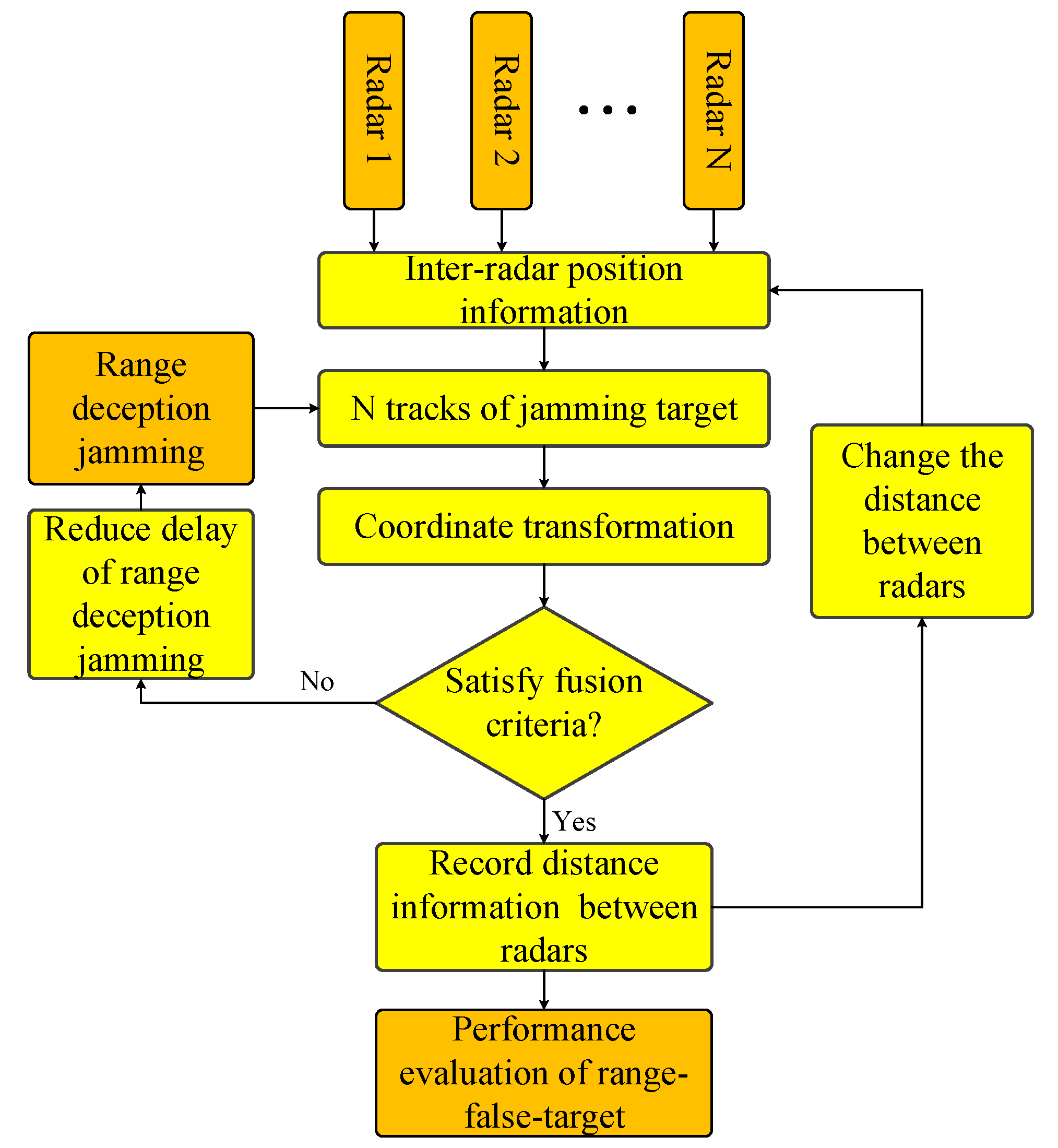
3. Range Deception Jamming Performance Evaluation Method for Ground-Based Radar Network

For the convenience of analysis, it is assumed that the ground-based network of radars is composed of three radars and that the range deception active jammer is located in the radar network detection coverage with a moving speed of v. From Figure 2, one can see that the position information of three radars can be described by using the longitude, latitude, and altitude information. The position of the s-th radar can be expressed as θ s L o , r a d a r , θ s L a , r a d a r , H r a d a r s , s = 1 , 2 , 3 , where θ s L o , r a d a r and θ s L a , r a d a r denote the longitude and latitude of the s-th radar, respectively, and H r a d a r s denotes the height of this radar where the height is represented from the land. The single range deception jammer position is denoted by θ L o , j a m , θ L a , j a m , h j a m . When the electromagnetic wave signal transmitted from the networking radars reaches the receiving antenna of the jammer, the jammer performs the amplitude and distance delay modulation on the received signal and then transmits the jamming signal, which is finally received by the networking radar system. It is assumed that the s-th radar detects a false target with a time delay of τ s + τ , where τ s ( s = 1 , 2 , 3 ) denotes the propagation time of the electromagnetic wave from the s-th radar to the jammer, and τ denotes the time delay corresponding to the jamming signal modulated by the jammer. Due to the difference in radar positions, the radar network will obtain three false target tracks. The jamming signal will successfully cheat the network radars if three tracks pass the homology detection in the radar network. Based on this, the jamming performance evaluation of the range deception jamming in the ground-based radar network system can be realized.

3.1. Radar Coordinate Transformation

When a radar network detects the jamming targets, each radar independently accomplishes the jamming signal detection. Thus, the detection information of each ground radar needs to be converted into the same coordinate system for subsequent information fusion. Therefore, this section first introduces the coordinate conversion of networked radar.
Considering that the Earth is approximated as a sphere, as shown in Figure 3, the Earth’s center is set as the origin point O e . The X e axis is set as the equatorial plane pointing to the prime meridian, the Z e axis is pointing to the north pole of the Earth, and the Y e axis is perpendicular to the X e axis and Z e axis, obeying the right-handed coordinate rule.
According to Figure 3, the 3D coordinates of the ground radar in the Earth-fixed coordinate system can be expressed as follows:
x e , r a d a r , s y e , r a d a r , s z e , r a d a r , s = R e + H r a d a r s cos θ L a , r a d a r s cos θ L o , r a d a r s R e + H r a d a r s cos θ L a , r a d a r s sin θ L o , r a d a r s R e + H r a d a r s sin θ L a , r a d a r s ,
where θ L o , r a d a r s , θ L a , r a d a r s , and H r a d a r s denote the longitude, latitude, and height of the s-th ground-based radar, respectively, and R e is the radius of the Earth. Then the coordinates of the jammer in the Earth-fixed coordinate system can be noted as follows:
x e , j a m y e , j a m z e , j a m = R e + h j a m cos θ L a , j a m cos θ L o , j a m R e + h j a m cos θ L a , j a m sin θ L o , j a m R e + h j a m sin θ L a , j a m ,
where θ L o , j a m , θ L a , j a m , and h j a m denote the longitude, latitude, and height of the jammer, respectively.
According to Equations (3) and (4), the coordinates of the jammer in the local coordinate system corresponding to the s-th radar can be obtained after performing the coordinate translation and rotation transformation, that is
x s , j a m y s , j a m z s , j a m = R × x e , j a m x e , r a d a r , s y e , j a m y e , r a d a r , s z e , j a m z e , r a d a r , s ,
where R denotes the rotational matrix, with the expression given by
R = 1 0 0 0 cos π 2 θ L a , r a d a r s sin π 2 θ L a , r a d a r s 0 sin π 2 θ L a , r a d a r s cos π 2 θ L a , r a d a r s × cos θ L o , r a d a r s + π 2 sin θ L o , r a d a r s + π 2 0 sin θ L o , r a d a r s + π 2 cos θ L o , r a d a r s + π 2 0 0 0 1
Therefore, according to Equations (3)–(6), the coordinates of the jammer in the local coordinate system established by the s-th ground-based radar can be expressed as follows:
x s , j a m y s , j a m z s , j a m = 1 0 0 0 cos π 2 θ L a , r a d a r s sin π 2 θ L a , r a d a r s 0 sin π 2 θ L a , r a d a r s cos π 2 θ L a , r a d a r s × cos θ L o , r a d a r s + π 2 sin θ L o , r a d a r s + π 2 0 sin θ L o , r a d a r s + π 2 cos θ L o , r a d a r s + π 2 0 0 0 1 × R e + h j a m cos θ L a , j a m cos θ L o , j a m R e + h j a m cos θ L a , j a m sin θ L o , j a m R e + h j a m sin θ L a , j a m R e + H r a d a r s cos θ L a , r a d a r s cos θ L a , r a d a r s R e + H r a d a r s cos θ L a , r a d a r s sin θ L a , r a d a r s R e + H r a d a r s sin θ L a , r a d a r s
Thus, the calculation results of range R s , elevation angle θ e l s , and azimuth angle θ a z i s of this jammer in the s-th radar coordinate system can be obtained:
R s = x s , j a m 2 + y s , j a m 2 + z s , j a m 2
θ e l s = arcsin z s , j a m x s , j a m 2 + y s , j a m 2 + z s , j a m 2
θ a z i s = arcsin y s , j a m x s , j a m 2 + y s , j a m 2 , x s , j a m > 0 , y s , j a m > 0 arcsin y s , j a m x s , j a m 2 + y s , j a m 2 + 360 ° , x s , j a m > 0 , y s , j a m < 0 arcsin y s , j a m x s , j a m 2 + y s , j a m 2 + 180 ° , o t h e r s
Based on the above coordinate transformation, the parameters of the jamming target can be estimated to obtain the trajectory information, and then the information fusion is implemented through the coordinate transformation.

3.2. Parameter Estimation

High-precision estimation of the elevation and azimuth angles and the range of an observed target can be achieved by using the single-pulse radar signal processing technology. This section introduces the parameter estimation of a single-pulse radar, which lays the foundation for the simulation and analysis of deception jamming evaluation in the next section.

3.2.1. Range Estimation

A monopulse radar generally transmits pulse signals with a large time–bandwidth product. Then the range pulse compression is used to estimate the target range. The expression s i s t in Equation (1) is transformed to the frequency domain by FFT, which can be expressed as follows:
S i s f r = A i a r f r B exp j π f r 2 γ exp j 2 π f r 2 R i s c ,
where A i represents the signal amplitude of the i-th echo, R i represents the i-th target range, and a r t represents the range window function. After performing the range pulse compression and IFFT, one has
S i s t = A i sin c B t 2 R i c ,
where the B denotes signal bandwidth. It can be seen from the above formula that the cell averaging constant false alarm rate (CA-CFAR) detection can be performed on the echo signal after range pulse compression in the time domain [16,17]. A certain CA-CFAR detection threshold is set based on the target detection performance requirements, so as to obtain the range unit that meets the threshold to realize the target range estimation.

3.2.2. Angle Estimation

A single-pulse radar receives an echo signal with several independent channels at the same time and compares these signals to obtain the angular error signal to accomplish the angle estimation [18]. The single-pulse angle measurement algorithm is widely used in modern precision tracking and measuring radar systems because it can obtain the angle information with the information of only one pulse and has the advantages of high angle measurement accuracy and strong anti-jamming ability.
The sum–difference beam angle measurement algorithm forms sum and difference beams at the receiving output [19,20]. The sum beam is the main lobe formed in the target direction, while the difference beam forms a null in the target direction. Angle estimation is completed through a certain value through the sum and difference beam ratio [21,22,23]. While the target deviates by the degree θ from the direction of the equal intensity signal, two beams for the deviation angle ± θ 0 of the equal intensity signal direction are generated in each coordinate plane. The echo signal at the receiving radar antenna can expressed be as follows:
P 1 t , θ = S i s t F θ 0 θ P 2 t , θ = S i s t F θ 0 + θ ,
where F θ represents the pattern function of radar transmitting antenna. The sum and difference signal can be obtained from Equation (13).

3.3. Interpolation Operation

Based on the above operations, a pulse radar can obtain the range and angle information of the moving target in a period of time, and then the moving target track can be obtained. However, because the ground-based pulse radar detects the target via airspace scanning, the target range data are relatively concentrated in a single circle and appear repeatedly in the scanning cycle. Therefore, it is necessary to interpolate the obtained track to obtain a uniformly distributed route for subsequent fusion processing.
Figure 4 shows the range information obtained by a signal-pulse radar during periodic detection, which is ununiformly sampled. Through the interpolation operation [20], the range information and the angle information can be evenly distributed by interpolation. Therefore, the moving target detected by a ground-based radar can be displayed as a non-uniform track in polar coordinates, as shown in Figure 5a. Figure 5b represents the uniform track after the data interpolation has been performed.

3.4. Track Fusion

After the jamming tracks are transformed to the same radar coordinate system, a statistical variance data fusion algorithm [24,25,26,27,28,29] can be applied to determine whether these tracks belong to the same target. Obviously, the target parameters including range, azimuth angle, and elevation angle estimated by a ground-based radar can be expressed as
R s = R s + ζ r s θ a s = θ a z i s + ζ a z i s θ e s = θ e l s + ζ e l s
where R s , θ a s , θ e s indicates the jammer position received by the s-th radar, R s denotes the slant range of the jammer, and θ a s and θ e s denote the azimuth and elevation angles, respectively. R s , θ a z i s , θ e l s are the accurate values of the jammer position, as given by Equations (6)–(8). ( ζ r s , ζ a z i s , ζ e l s ) represent the measurement errors of the s-th radar. Assume that the measurement errors obey the normal distribution ζ r s ~ 0 , σ r s 2 , ζ a z i s ~ 0 , σ a s 2 , and ζ e l s ~ 0 , σ e l 2 . Then the jammer target position model in the Cartesian coordinate system received by s-th radar can be obtained:
X s = R s cos θ e s cos θ a s = ( R s + ζ r s ) cos ( θ e l s + ζ e l s ) cos ( θ a z i s + ζ a z i s ) Y s = R s cos θ e s sin θ a s = ( R s + ζ r s ) cos ( θ e l s + ζ e l s ) sin ( θ a z i s + ζ a z i s ) Z s = R s sin θ e s = ( R s + ζ r s ) sin ( θ e l s + ζ e l s )
Assuming that the jammer target parameters recorded by radar 1 and radar 2 are, respectively, expressed as X A , Y A , Z A and X B , Y B , Z B in the same coordinate system, the position deviation can be expressed as follows:
Δ X = X A X B = R s A cos θ e s A cos θ a s A R s B cos θ e s B cos θ a s B = ( R A + ζ r A ) cos ( θ e l A + ζ e l A ) cos ( θ a z i A + ζ a z i A ) ( R B + ζ r B ) cos ( θ e l B + ζ e l B ) cos ( θ a z i B + ζ a z i B )
Δ Y = Y A Y B = R s A cos θ e s A sin θ a s A R s B cos θ e s B sin θ a s B = ( R A + ζ r A ) cos ( θ e l A + ζ e l A ) sin ( θ a z i A + ζ a z i A ) ( R B + ζ r B ) cos ( θ e l B + ζ e l B ) sin ( θ a z i B + ζ a z i B )
Δ Z = Z A Z B = R s A sin θ e s A R s B sin θ e s B = ( R A + ζ r A ) sin ( θ e l A + ζ e l A ) ( R B + ζ r B ) sin ( θ e l B + ζ e l B )
Let f X R , ζ = Δ X , where R = R A , θ e l A , θ a z i A , R B , θ e l B , θ a z i B T , ζ = ζ r A , ζ e l A , ζ a z i A , ζ r B , ζ e l B , ζ a z i B T . Then the first-order Taylor expansion of the function f X R , ζ at the point ζ = 0 can be expressed as
f X R , ζ f X R , ζ ' + f X R , ζ ' ζ ζ ζ ' ,
where ζ ' = 0 , 0 , 0 , 0 , 0 , 0 T , with the expressions of f X R , ζ ' and f X R , ζ ' ζ ζ ζ ' given by
f X R , ζ ' = R A cos θ e l A cos θ a z i A R B cos θ e l B cos θ a z i B
f X R , ζ ' ζ ζ ζ ' = cos θ e l A cos θ a z i A ζ r A R A sin θ e l A cos θ a z i A ζ e l A R A cos θ e l A sin θ a z i A ζ a z i A cos θ e l B sin θ a z i B ζ r B + R B sin θ e l B cos θ a z i B ζ e l B + R B cos θ e l B sin θ a z i B ζ a z i B
The position deviation in the X direction can be approximated as follows:
Δ X = f X R , ζ = R A cos θ e l A cos θ a z i A R B cos θ e l B cos θ a z i B + cos θ e l A cos θ a z i A ζ r A R A sin θ e l A cos θ a z i A ζ e l A R A cos θ e l A sin θ a z i A ζ a z i A cos θ e l B cos θ a z i B ζ r B + R B sin θ e l B cos θ a z i B ζ e l B + R B cos θ e l B sin θ a z i B ζ a z i B
Similarly, the position deviations in the Y and Z directions can be noted as follows:
Δ Y = f Y R , ζ = R A cos θ e l A sin θ a z i A R B cos θ e l B sin θ a z i B + cos θ e l A sin θ a z i A ζ r A R A sin θ e l A sin θ a z i A ζ e l A + R A cos θ e l A cos θ a z i A ζ a z i A cos θ e l B sin θ a z i B ζ r B + R B sin θ e l B sin θ a z i B ζ e l B R B cos θ e l B cos θ a z i B ζ a z i B
Δ Z = f Z R , ζ = R A sin θ e l A R B sin θ e l B + sin θ e l A ζ r A + R A cos θ e l A ζ e l A sin θ e l B ζ r B R B cos θ e l B ζ e l B
It is considered that
R A cos θ e l A cos θ a z i A R B cos θ e l B cos θ a z i B = 0
Then, Δ X in (18) can be further expressed as follows:
f X ζ = cos θ e l A cos θ a z i A ζ r A R A sin θ e l A cos θ a z i A ζ e l A R A cos θ e l A sin θ a z i A ζ a z i A cos θ e l B cos θ a z i B ζ r B + R B sin θ e l B cos θ a z i B ζ e l B + R B cos θ e l B sin θ a z i B ζ a z i B
According to the property of the normal distribution, the function f X ζ still obeys the normal distribution and E f X ζ = 0 . In addition, its variance can be expressed as follows:
V a r f X ζ = ( cos θ e l A cos θ a z i A ) 2 V a r ( ζ r A ) + ( R A sin θ e l A cos θ a z i A ) 2 V a r ( ζ e l A ) + ( R A cos θ e l A sin θ a z i A ) 2 V a r ( ζ a z i A ) + ( cos θ e l B cos θ a z i B ) 2 V a r ( ζ r B ) + ( R B sin θ e l B cos θ a z i B ) 2 V a r ( ζ e l B ) + ( R B cos θ e l B sin θ a z i B ) 2 V a r ( ζ a z i B ) ,
where V a r represents the variance operation. According to the confidence interval of the normal distribution, one has
0.997 P f X ζ 3 σ f X ζ = P Δ X 3 σ f X ζ ,
where σ represents standard deviation. From Equation (27), one can see that if the position deviation in the X-axis direction exceeds this range, the probability that these two sets of parameters are not from the same jammer target is greater than 0.997. Similarly, the position deviation distribution functions along Y-axis and Z-axis directions can be obtained, with the variance expressed as follows:
V a r f Y ζ = ( cos θ e l A sin θ a z i A ) 2 V a r ( ζ r A ) + ( R A sin θ e l A sin θ a z i A ) 2 V a r ( ζ e l A ) + ( R A cos θ e l A cos θ a z i A ) 2 V a r ( ζ a z i A ) + ( cos θ e l B sin θ a z i B ) 2 V a r ( ζ r B ) + ( R B sin θ e l B sin θ a z i B ) 2 V a r ( ζ e l B ) + ( R B cos θ e l B cos θ a z i B ) 2 V a r ( ζ a z i B )
V a r f Z ζ = ( sin θ e l A ) 2 V a r ( ζ r A ) + ( R A cos θ e l A ) 2 V a r ( ζ e l A ) + ( sin θ e l B ) 2 V a r ( ζ r B ) + ( R B cos θ e l B ) 2 V a r ( ζ e l B )
The fusion criterion can be noted as follows:
Δ X 3 σ f X ζ Δ Y 3 σ f Y ζ Δ Z 3 σ f Z ζ
When the position deviations in the three directions satisfy Equation (31), these jamming tracks can be considered to come from the same target. If any of these three conditions is not satisfied, these tracks do not belong to the same target and the track fusion fails. Based on this fusion criterion, the fusion rate among different tracks can be calculated. For multiple radars, the fused tracks need to be fused with other tracks again.
The complete flowchart of the proposed jamming effectiveness evaluation algorithm is shown in Figure 6.
According to the above flowchart, the processing steps of the proposed evaluation method are given as follows:
Step 1: Set a single range deception jammer and a certain range delay, and simulate the radar network composed of N radars to obtain N jamming tracks.
Step 2: Use the coordinate transformation in Equation (7) to transform these N trajectories into the same coordinate system.
Step 3: Perform the track fusion on multiple tracks in the same coordinate system. If the fusion criterion in Equation (31) is satisfied, the range deception jamming is successful, and the inter-radar distance information is recorded.
Step 4: Change the distance between radars and repeat the experiment to obtain the deception jamming range delay boundary which satisfies the fusion criterion under different radar spacing conditions.

4. Simulation Experiment Analysis

In this section, a radar network consisting of three radars is set up to simulate the jamming tracks. The system parameters of these three radars are listed in Table 1 and Table 2. The initial position of the target is set as 121°E, 31°N, and the initial target height is set as 5 km. The normal target speed is 30 m/s, and the target speed direction points to the northwest. In addition, the heights of these three radars from the ground are set as 30 m.
Figure 7 shows the results of the detection of the jammer target by radar 1 and radar 2 under the coordinate system belonging to radar 3, where the green line (plus) is the target trajectory detected by radar 1 and the blue line (dotted) is the target trajectory detected by radar 2. In addition, the red line (asterisked) is the target track detected by radar 3, where the jamming range delay is set as 5 km. From Figure 7, it is clearly seen that the false target tracks do not overlap, indicating that the jamming signal fails to interfere with this ground-based radar network composed of three radars. Therefore, the jamming range delay should be reasonably designed in order to make the jamming signal successfully disturb this radar network.

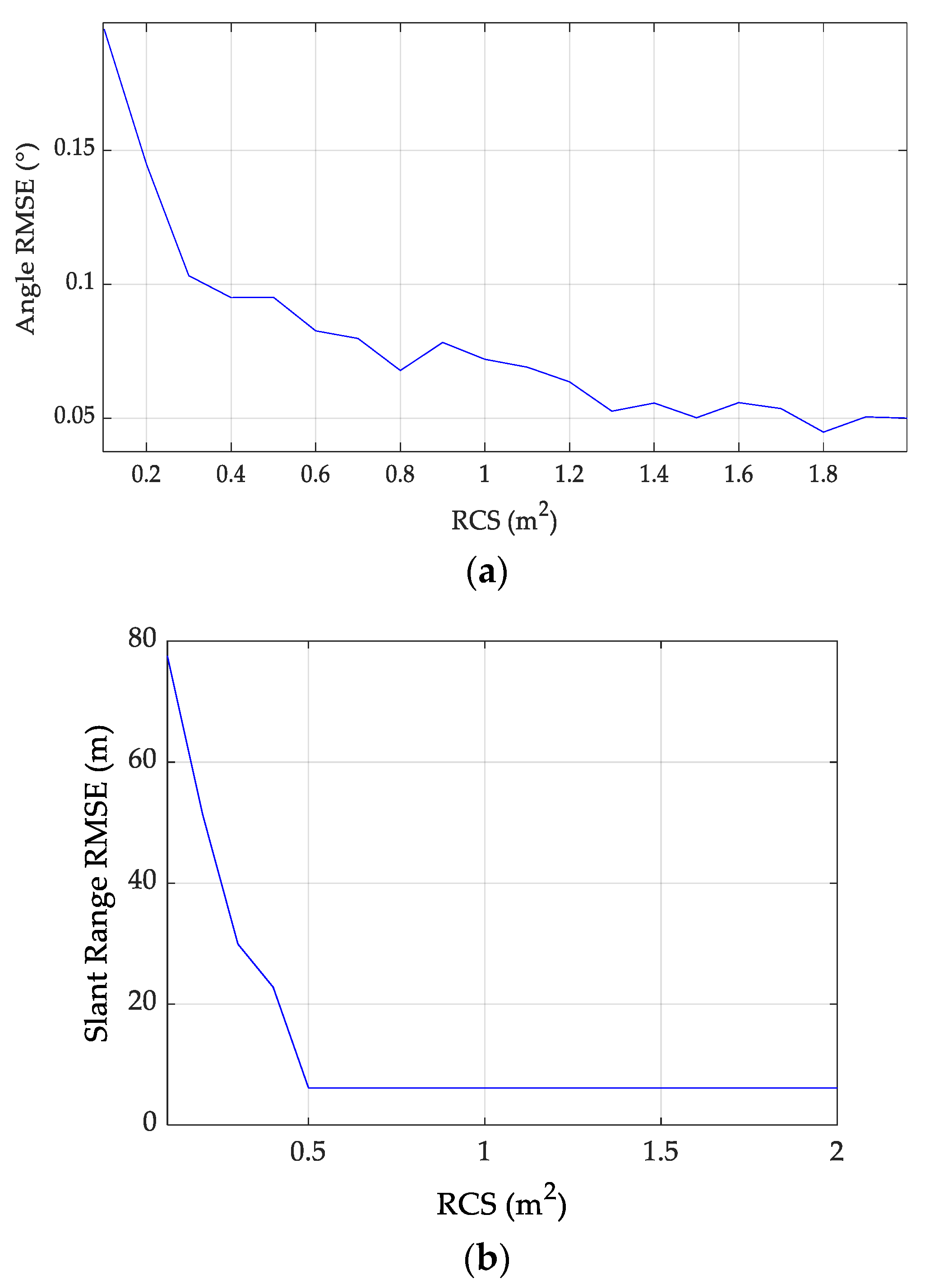
4.1. Simulation Analysis of Radar Slant Range and Angle Measurement Errors

From the analysis in Section 3.2, we can know that the appropriate angle and slant range variance values need to be set in advance to ensure the effective fusion of jamming tracks in the same coordinate system, which can be estimated via the simulation results. In the following, the radar slant range measurement error and angle measurement error are evaluated via the Monte Carlo experiments, where 1000-repetition experiments are performed for every given target RCS [16,17]. The relation of the root mean squared error (RMSE) of the slant range error and angle error versus target RCS can be obtained. The other radar and jamming target parameters are listed in Table 1 and Table 2, respectively. Figure 8 shows the simulation results, from which one can see that the estimation accuracy of the target angle and range is gradually improved with the increase in the target’s RCS. When the target RCS is within the range of 0.5 to 2, the signal-to-noise ratio (SNR) is relatively high, and the range resolution of the radar system is 150 m, which is related to the range time sampling. In all repetitive experiments, the peak value of the target echo signal is basically at the same discrete range resolution unit under the detection threshold of 13 dB. Therefore, the slant range measurement accuracy is basically not affected by the change in the target RCS with the range of 0.5 to 2 as shown in Figure 8b.
Based on similar experiments, the slant range error and angle error of three radars with different parameters were simulated and the RMSE information was obtained, as listed in Table 3. The RMSE information can be used in the fusion criteria as the standard deviation of error.

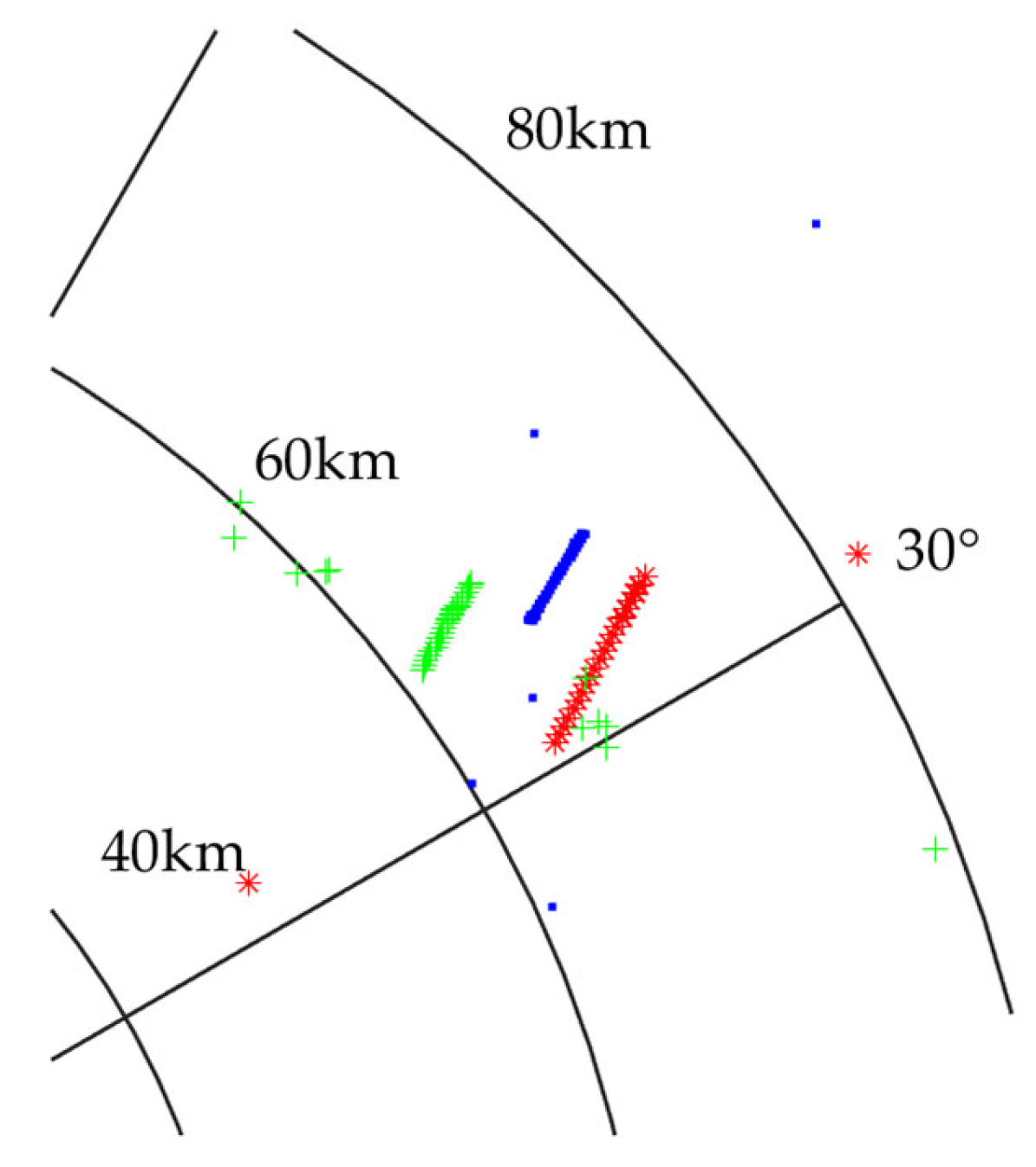
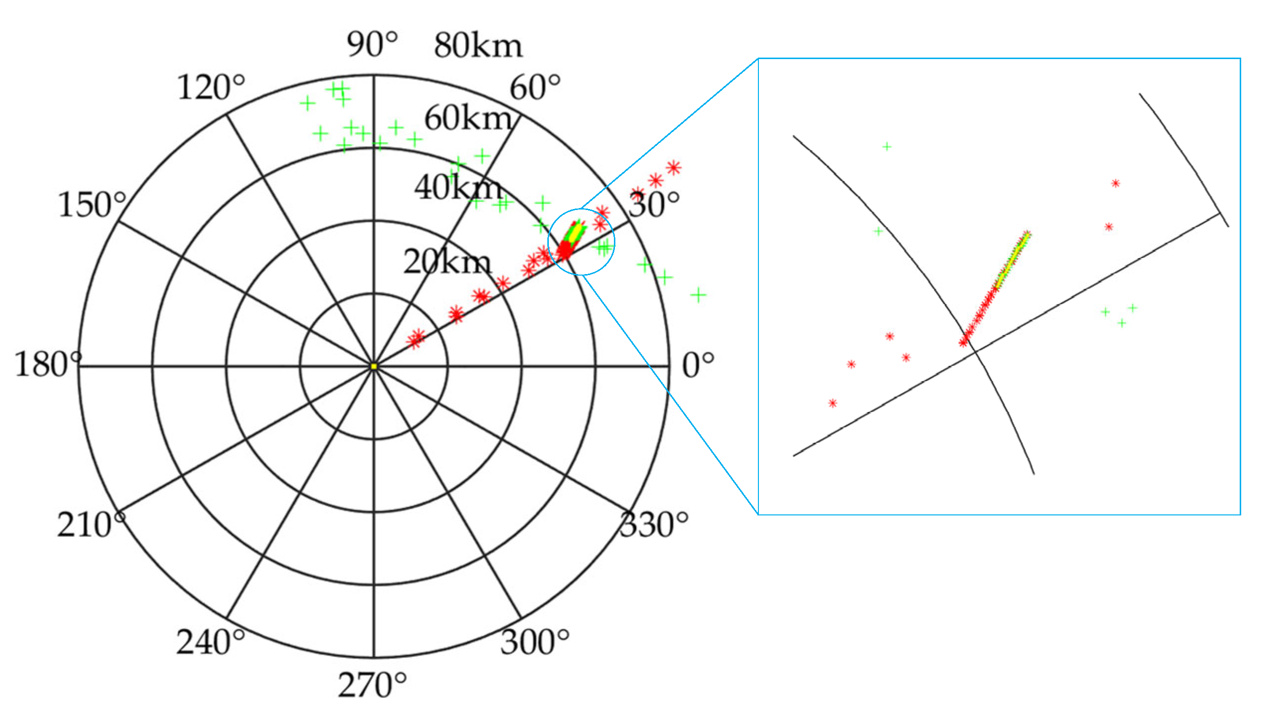
4.2. True Target Track Fusion Analysis

Considering that a true target track will be completely coincident after CFAR detection is performed by several radars, in order to verify the validity of the fusion criterion, the fusion simulation of the true target track without adding the range deception jamming delay is performed in the following.
To facilitate analysis, two detection tracks of radar 1 and radar 3 are taken for fusion processing, where the range deception jamming delay is set as 0 km. According to the angle and range estimation results in Figure 8 and Table 3, the estimation error standard deviation can be noted as follows:
σ ζ r A = σ ζ r B = 3.8 m σ ζ e l A = σ ζ a z i A = 0.045 σ ζ e l B = σ ζ a z i B = 0.1
Based on Equation (32), Figure 8 shows the fusion results of true target tracks recorded by two ground-based radars. The green line (plus) is the target track detected by radar 1 under the local coordinate of the radar 3 system, and the red line (asterisked) is the target track detected by radar 3. The yellow line (dotted) is the track point that satisfies the fusion criterion given in Equation (31). It can be seen from Figure 9 that the motion trajectories received by two radars are successfully associated after the fusion criterion is applied. In addition, the noise traces received by radar 3 can also be well eliminated according to the fusion criterion. For a true target, the fusion rate of the target track detected by radar 1 and the target track detected by radar 3 is statistically about 90.2%, which indicates that the true target obviously satisfies the track fusion requirements. The fusion rate represents the ratio between the track points (yellow line) that satisfy the fusion criteria and the total number of track points (green line).

4.3. Jamming Range Delay Boundary Analysis

In order to evaluate the performance of range deception jamming, the jamming range delay boundary is analyzed by setting radar networks with different numbers and positions. Then some conclusions are summarized through repeated experiments.

4.3.1. Two-Radar System

In this simulation, for convenience of analysis, two tracks of radar 1 and radar 3 are applied to realize the fusion processing and performance analysis, where the local coordinate system of radar 3 is taken as the reference coordinate system. Assume that the position of radar 1 is unchanged, and the position of radar 3 is adjusted to 120.8° E, 30.5° N, which is about 22 km away from radar 1. Figure 10 shows the fusion results when the range delay is set as 10 km, 20 km, 30 km, and 40 km where the fusion rate is statistically 82.6%, 72.3%, 60.0%, and 25.4% in these four cases. If the track fusion rate threshold is set as 80%, one can see that these two jamming false target tracks are successfully fused when the range delay is 10 km, and the target track is not effectively fused when the range delay is increased to 20 km, 30 km, and 40 km, indicating that the delay boundary of these two radars system is between 10 km and 20 km.
By adjusting the distance between radar 1 and radar 3, the jamming range delay boundary at different radar positions can be obtained, as listed in Table 4. In addition, the change in the jamming range delay boundary under different radar and jammer target distance conditions is analyzed by changing the initial distance between the fixed radar and the jammer target.
Condition 1: The distance between the jammer target and radar 1 is 38.2 km, where the coordinates of the jammer are (E120.9°, N31°, 5 km). (a) When the distance between these two radars is 89 km, the jamming range delay boundary is 0.4~0.5 km. (b) When the distance between the two radars is 45.4 km, the jamming range delay boundary is 5~10 km. (c) When the distance between the two radars is 22 km, the jamming range delay boundary is 10~20 km. (d) when the distance between the two radars is 11 km, the jamming range delay boundary is 35~40 km.
Condition 2: The distance between the jammer target and radar 1 is 72.8 km, where the coordinates of the jammer are (E121.3°, N31.5°, 5 km). (a) When the distance between two radars is 53.6 km, the jamming range delay boundary is between 3 and 5 km. (b) When the distance between two radars is 33 km, the jamming range delay boundary is between 5 and 10 km. (c) When the distance between two radars is 22 km, the jamming range delay boundary is between 10 and 15 km.
From Table 4, it can be concluded that the range delay boundary decreases with the increase in distance between two radars when the distance between the radar and the target remains constant. In addition, the range delay boundary corresponding to the range deception jamming increases with the increase in distance between the radar and the target.

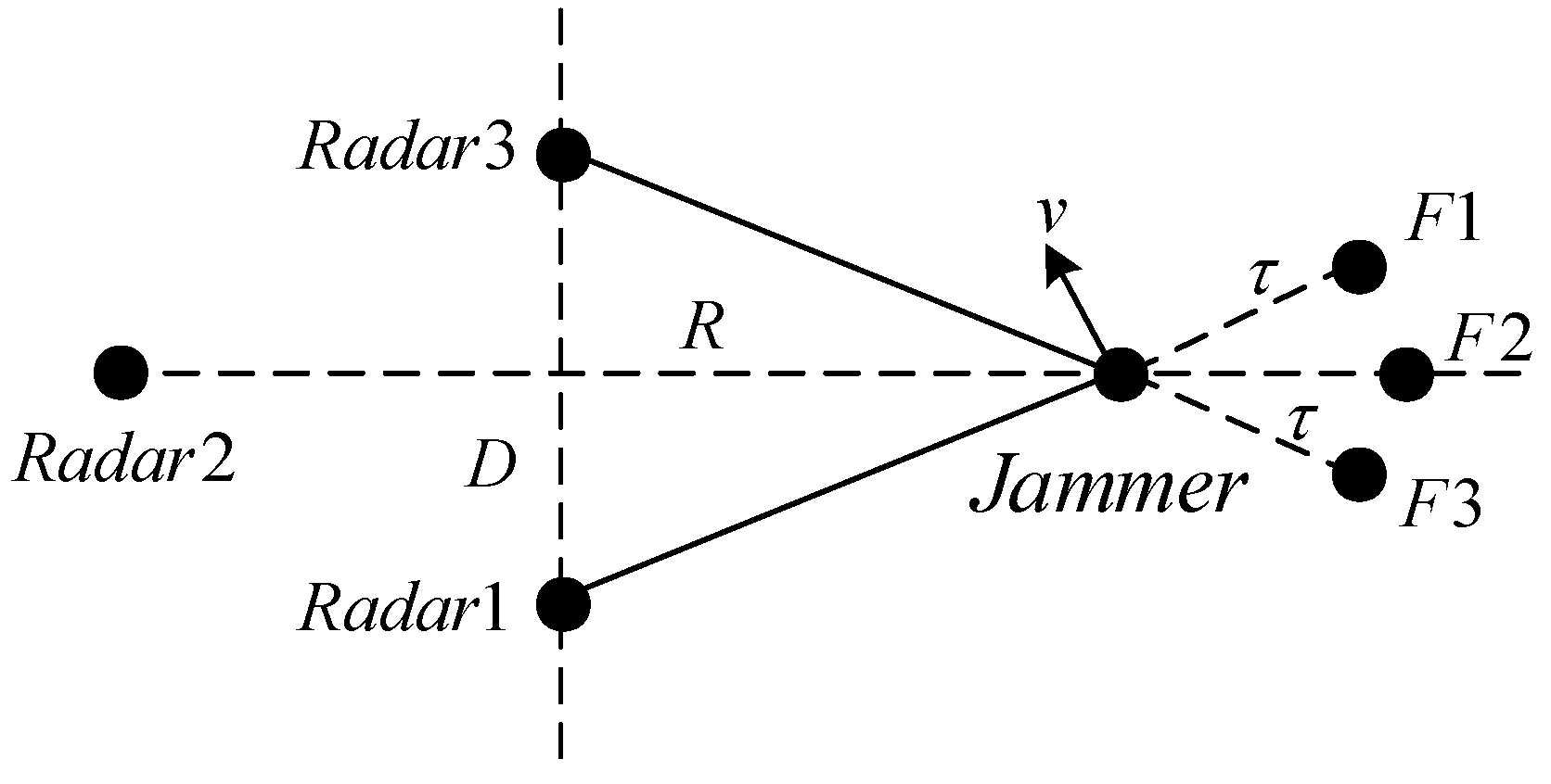
4.3.2. Three-Radar System

In this simulation, three tracks of radar 1, radar 2, and radar 3 are taken to accomplish the track fusion processing, where the local coordinate system of radar 3 is taken as the reference coordinate system. The distribution diagram and the parameter result of these three radars are shown in Figure 11 and listed in Table 5, respectively, where the radar system parameters of radar 1 and radar 3 are consistent. The tracks observed by radar 1 and radar 2 are converted to the local coordinate system of radar 3 and fused with radar 3 detection tracks, and then two fusion tracks can be obtained. Finally, a second fusion is required with these two fusion tracks, so as to obtain the final fusion rate.
Table 6 shows the fusion rate of range deception jamming target trajectory detected by the three-radar system, where the distance R in Figure 10 is set as 67.7 km and 86.6 km, where the coordinates of the jammer are (E121.3°, N31.1°, 5 km) and (E121.5°, N31.1°, 5 km), respectively. It can be concluded that as the distance between the jammer and the radar system increases, the track fusion rate increases. By comparison with the jamming evaluation result of the two-radar system, it can be seen that this three-radar system has lower track fusion rates and better anti-jamming capabilities.

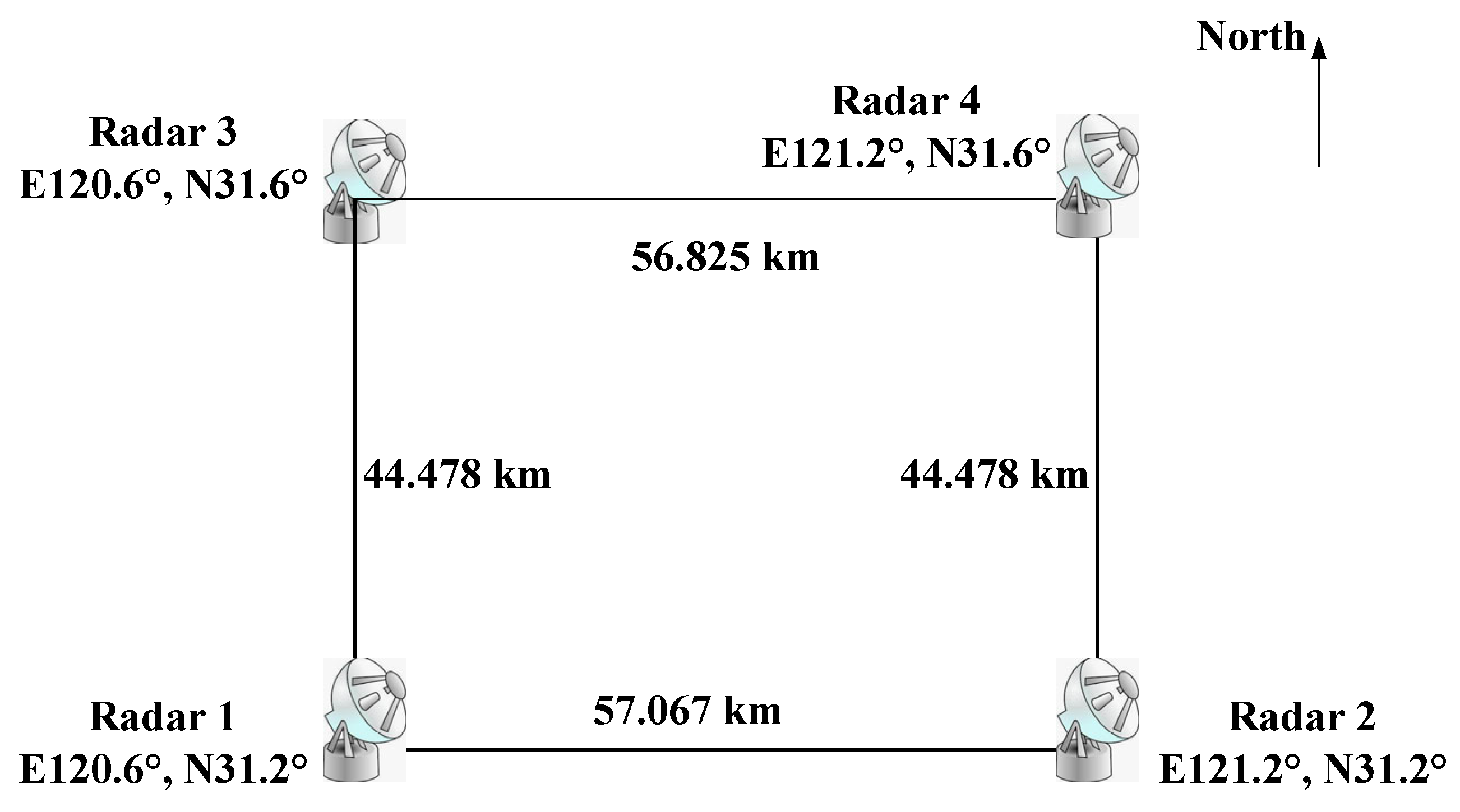
4.3.3. Four-Radar System

In the following, the four tracks of radar 1, radar 2, radar 3, and radar 4 are taken to accomplish the fusion operation, and the local coordinate system of radar 3 is taken as the reference coordinate system. The parameter settings of these four radars are shown in Table 7, where the positions of these four radars are distributed as shown in Figure 12. The track fusion is still carried out in the coordinate system of radar 3, and the distance between radar 3 and the observed jamming target is 76.8 km where the coordinates of the jammer are (E121°, N32°, 5 km), with the fusion rate results shown in Table 8. It can be seen from the table that when the jamming range deception delay is small enough, the tracks detected by the four radars have a high fusion rate under certain fusion criteria, which indicates that the jamming target can successfully cheat the radar system. At the same time, compared with the fusion results in the two-radar system and three-radar system, it is more difficult for the four-radar system to be interfered with by the range deception jamming target (see the compared results in Table 4, Table 6 and Table 8).

5. Discussion

There are other forms of deception jamming, including cover pulse jamming and velocity deception jamming [22]. Cover pulse jamming creates a noise pulse when a radar signal is received and conceals any aircraft flying behind the jammer with a block of noise. Velocity deception jamming changes the velocity the radar detects by changing the Doppler shift of the transmitted signal through DRFM. Both cover pulse jamming and velocity deception jamming can easily deceive monostatic radars and are similar to range deception jamming. For multistatic radar systems, cover pulse jamming requires the generation of noise with sufficient energy and is also related to the angle between the radars and the target. Velocity deception jamming requires varying different Doppler frequency shifts based on the angle between the target and each radar to achieve deception.

6. Conclusions

This paper mainly analyzes the boundary of the range deception jammer in order to successfully interfere with the radar network. This paper first establishes the coordinate system conversion relationship among different radars and then introduces a statistical variance data fusion rule for trajectory fusion. Finally, the jamming range delay boundary is obtained under different radar positions and different numbers of radars by virtue of the fusion of the jamming tracks for the network radars. The simulation results show the following: (1) The tracks can be well fused without the range deception delay. (2) For a two-radar system, the range delay boundary decreases with the increase in distance between two radars when the distance between the radar and the jammer remains constant. In addition, the range delay boundary corresponding to the range deception jamming increases with the increase in distance between the radar and the jammer. (3) Compared with the two-radar system, three- and four-radar systems have lower track fusion rates and better anti-jamming capabilities. (4) As the number of radars increases, the range delay boundary becomes relatively small, making it more difficult for jammers to interfere with networked radars. (5) The range delay boundary is closely related to the configuration of the networked radars and the location of the jammer. Therefore, it is concluded that the range deception jamming delay boundary decreases with the increase in the distances with respect to different radars, which exhibits a certain guiding significance for the actual engineering of range deception jamming in a radar network system.

Author Contributions

Conceptualization, Q.L. and P.H.; methodology, Q.L.; software, Q.L. and L.W.; validation, Q.L., D.W. and H.X.; formal analysis, P.H. and X.L.; investigation, Y.S.; resources, P.H.; data curation, Q.L.; writing—original draft preparation, P.H.; writing—review and editing, Q.L.; visualization, Q.L.; supervision, D.W. and G.L.; project administration, P.H.; funding acquisition, P.H. All authors have read and agreed to the published version of the manuscript.

Funding

This work was supported in part by the National Natural Science Foundation Program of China under Grant 62171272, and in part by USCAST2021-15, USCAST2022-21, and SAST2019-071 (Corresponding Author: Penghui Huang).

Data Availability Statement

Not applicable.

Acknowledgments

The author would like to thank all anonymous reviewers and editors for their comments and suggestions.

Conflicts of Interest

The authors declare no conflict of interest.

Nomenclature

AcronymsDescription
ECMelectronic countermeasure
ECCMelectronic counter-countermeasure
DRFMdigital radio frequency memory
RCS radar cross-section
PRFpulse repetition frequency
CFARconstant false alarm rate
CA-CFARcell averaging constant false alarm rate
RMSEroot mean squared error
FFTfast Fourier transform
IFFTinverse fast Fourier transform

References

  1. Zhu, X.-L. Design Efficiency Evaluation Index System of Radar Networking System. Shipboard Electron. Countermeas. 2019, 42, 48–51. [Google Scholar]
  2. Skolnik, M.I. Radar Handbook, 3rd ed.; McGraw-Hill: New York, NY, USA, 2008. [Google Scholar]
  3. Tao, F.; Kojima, N. A new method for fabricating cell-embedded ECM capsules and ECM-loaded spheroids. In Proceedings of the 2015 International Symposium on Micro-NanoMechatronics and Human Science (MHS), Nagoya, Japan, 23–25 November 2015; pp. 1–3. [Google Scholar]
  4. Saha, P.K.; Shekhar, S.; Laxmi, V.; Thakura, P.R. Improved Speed Response of ECM Drive Using Antiwindup Concept. In Proceedings of the 2019 3rd International Conference on Electronics, Communication and Aerospace Technology (ICECA), Coimbatore, India, 12–14 June 2019; pp. 286–289. [Google Scholar]
  5. Ji, Z.; Wang, G.; Zhang, X.; Sun, D. Technique of anti-multi-range-false-target jamming for radar network based on double discrimination. In Proceedings of the 2016 CIE International Conference on Radar, Guangzhou, China, 10–13 October 2016; pp. 1–5. [Google Scholar]
  6. Akhtar, J. Orthogonal block coded ECCM schemes against repeat radar jammers. IEEE Trans. Aerosp. Electron. Syst. 2009, 45, 1218–1226. [Google Scholar] [CrossRef]
  7. Zhao, Z.C.; Wang, X.S.; Xiao, S.P. Cooperative deception jamming against radar network using a team of UAVs. In Proceedings of the 2009 IET International Radar Conference, Guilin, China, 20–22 April 2009; pp. 1–4. [Google Scholar]
  8. Huang, C.; Chen, Z.; Duan, R. Novel discrimination algorithm for deceptive jamming in polarimetric radar. Proc. Int. Conf. Inf. Technol. Softw. Eng. 2013, 210, 359–365. [Google Scholar]
  9. Yang, Y.; Da, K.; Zhu, Y.; Xiang, S.; Fu, Q. Consensus based target tracking against deception jamming in distributed radar networks. IET Radar Sonar Navig. 2023. ahead of print. [Google Scholar] [CrossRef]
  10. Liang, X.; Zhang, Q.; Luo, Y. The research of deceptive jamming of missile warhead based on micro-Doppler effect. J. Proj. Rocket. Missiles Guid. 2011, 31, 56–67. [Google Scholar]
  11. Zhao, S.; Liu, N.; Zhang, L.; Zhou, Y.; Li, Q. Discrimination of deception targets in multistatic radar based on clustering analysis. IEEE Sens. J. 2016, 16, 2500–2508. [Google Scholar] [CrossRef]
  12. Wang, Z.; Li, T.; Liu, J. Radar Jamming Effect Analysis Based on Bayesian Inference Network with Adaptive Clustering. IEEE Sens. J. 2021, 21, 15153–15160. [Google Scholar] [CrossRef]
  13. Lv, B.; Song, Y.; Zhou, C.-Y. Study of multistatic radar against velocity-deception jamming. In Proceedings of the 2011 International Conference on Electronics, Communications and Control (ICECC), Ningbo, China, 9–11 September 2011; pp. 1044–1047. [Google Scholar]
  14. Zhang, S.; Zhou, Y.; Zhang, L.; Zhang, Q.; Du, L. Target Detection for Multistatic Radar in the Presence of Deception Jamming. IEEE Sens. J. 2021, 21, 8130–8141. [Google Scholar] [CrossRef]
  15. Zhao, S.; Zhang, L.; Zhou, Y.; Liu, N. Signal fusion-based algorithms to discriminate between radar targets and deception jamming in distributed multiple-radar architectures. IEEE Sens. J. 2015, 15, 6697–6706. [Google Scholar] [CrossRef]
  16. Cui, Z.; Hou, Z.; Yang, H.; Liu, N.; Cao, Z. A CFAR Target-Detection Method Based on Superpixel Statistical Modeling. IEEE Geosci. Remote Sens. Lett. 2021, 18, 1605–1609. [Google Scholar] [CrossRef]
  17. Kuang, C.; Wang, C.; Wen, B.; Hou, Y.; Lai, Y. An Improved CA-CFAR Method for Ship Target Detection in Strong Clutter Using UHF Radar. IEEE Signal Process. Lett. 2020, 27, 1445–1449. [Google Scholar] [CrossRef]
  18. Oraizi, H.; Fallahpour, M. Sum, Difference and Shaped Beam Pattern Synthesis by Non-Uniform Spacing and Phase Control. IEEE Trans. Antennas Propag. 2011, 59, 4505–4511. [Google Scholar] [CrossRef]
  19. Fan, X.; Liang, J.; Jing, Y.; So, H.C.; Geng, Q.; Zhao, X. Sum/Difference Pattern Synthesis with Dynamic Range Ratio Control for Arbitrary Arrays. IEEE Trans. Antennas Propag. 2022, 70, 1940–1953. [Google Scholar] [CrossRef]
  20. Han, X.; He, H.; Zhang, Q.; Yang, L.; He, Y.; Li, Z. Main-Lobe Jamming Suppression Method for Phased Array Netted Radar Based on MSNR-BSS. IEEE Sens. J. 2022, 22, 22972–22984. [Google Scholar] [CrossRef]
  21. Bar-Shalom, Y.; Willett, P.K.; Tian, X. Tracking and Data Fusion: A Handbook of Algorithms; YBS Publishing: Storrs, CT, USA, 2011. [Google Scholar]
  22. Nouri, M.; Mivehchy, M.; Sabahi, M.F. Novel anti-deception jamming method by measuring phase noise of oscillators in LFMCW tracking radar sensor networks. IEEE Access 2017, 5, 11455–11467. [Google Scholar] [CrossRef]
  23. Chen, H.; Kirubarajan, T. Performance limits of track-to-track fusion versus centralized estimation: Theory and application. IEEE Trans. Aerosp. Electron. Syst. 2003, 39, 386–400. [Google Scholar] [CrossRef]
  24. Gao, X.; Chen, J.; Tao, D.; Li, X. Multi-sensor centralized fusion without measurement noise covariance by variational Bayesian approximation. IEEE Trans. Aerosp. Electron. Syst. 2011, 47, 272–718. [Google Scholar] [CrossRef]
  25. Feng, X.; Zhao, Y.-N.; Zhao, Z.-F.; Zhou, Z.-Q. Cognitive tracking waveform design based on multiple model interaction and measurement information fusion. IEEE Access 2018, 6, 30680–30690. [Google Scholar] [CrossRef]
  26. Chen, Z.; Wang, G.; Guan, C.; Tan, S. A Biased Track Association Algorithm Based Modified Global Nearest Neighbor Algorithm. J. Proj. Rocket. Missiles Guid. 2012, 32, 167–170. [Google Scholar]
  27. You, H. Radar Data Processing and Application, 1st ed.; Publishing House of Electronics Industry Press: Beijing, China, 2009. [Google Scholar]
  28. Zhao, Y.-L.; Wang, X.-S.; Wang, G.-Y.; Liu, Y.-H.; Luo, J. Tracking Technique for Radar Network in the Presence of Multi-Range-False-Target Deception Jamming. Acta Electron. Sin. 2007, 35, 454–457. [Google Scholar]
  29. Rao, B.; Gu, Z.; Nie, Y. Deception Approach to Track-to-Track Radar Fusion Using Noncoherent Dual-Source Jamming. IEEE Access 2020, 8, 50843–50858. [Google Scholar] [CrossRef]
Figure 1. Deception jamming deceives radars based on DRFM.
Electronics 12 01614 g001
Figure 2. Geometric position distribution of three radars and a jammer.
Electronics 12 01614 g002
Figure 3. Earth-fixed coordinate system and radar local coordinate system.
Electronics 12 01614 g003
Figure 4. The range transformation of jamming with an enlarged view of radar main-lobe pulse sequence in a circle.
Electronics 12 01614 g004
Figure 5. The moving target track detected by ground-based radar in polar coordinates: (a) before interpolation; (b) after interpolation.
Electronics 12 01614 g005
Figure 6. Flowchart for the jamming performance evaluation.
Electronics 12 01614 g006
Figure 7. Three tracks in the radar 3 coordinate system, where green line (plus) is detected by radar 1, blue line (dotted) is detected by radar 2, and red line (asterisked) is detected by radar 3.
Electronics 12 01614 g007
Figure 8. Target angle and slant range error estimation results: (a) RMSE of angle versus target RCS; (b) RMSE of slant range versus target RCS.
Electronics 12 01614 g008
Figure 9. True target fusion results with a jamming range delay of 0 km including overall rendering and partly enlarged view, where green line (plus) denotes the track detected by radar 1, red line (asterisked) is detected by radar 3, and yellow line (dotted) is the target track that satisfies the fusion criterion.
Electronics 12 01614 g009
Figure 10. Fusion performance analysis in a two-radar system: (a) Target track fusion results when the jamming range delay is set as 10 km; (b) target track fusion results when the jamming range delay is set as 20 km; (c) jamming range delay is 30 km; (d) jamming range delay is 40 km (green line (plus) is detected by radar 1, red line (asterisked) is detected by radar 3, yellow line (dotted) is track that satisfies fusion criterion).
Electronics 12 01614 g010
Figure 11. Distribution diagram of three radars.
Electronics 12 01614 g011
Figure 12. Distribution diagram of four radars.
Electronics 12 01614 g012
Table 1. Radar network parameters.
PositionCarrier FrequencyRCS
(m2)
Rotating Velocity
(r/min)
Antenna
Azimuth Size (m)
Radar 1E120.8,
N30.7
800 MHz1.81887.3
Radar 2E120.5,
N31.1
1.3 GHz0.97866.3
Radar 3E120.6,
N31.5
3 GHz0.92544.3
Table 2. Radar system parameters.
ParametersValue
Radar peak power150 kW
Transmit signal bandwidth1 MHz
PRF500 Hz
Duty ratio0.07
Antenna range size4.3 m
System loss7 dB
Noise factor3 dB
Table 3. RMSE of range and angle of three radars.
Carrier
Frequency
RCS
(m2)
Antenna
Azimuth Size (m)
RMSE of Slant Range (m)RMSE of Angle (°)
Radar 1800 MHz1.8187.33.80.045
Radar 21.3 GHz0.9786.33.80.08
Radar 33 GHz0.9254.33.80.10
Table 4. Jamming performance evaluation results of a ground-based radar network (two radars).
Distance of Fixed Radar from Target (km)Two-Radar Distance
(km)
Jamming Range Delay
(km)
Fusion RateSuccessful Fusion
38.21.12083.5%
4093.5%
6082.9%
8080.1%
8.92087.9%
4083.1%
6077.3%×
8070.3%×
112087.2%
3090.2%
3576.6%×
4076.6%×
16.71087.3%
2077.5%×
3066.8%×
4057.9%×
221082.6%
2072.3%×
3060.0%×
4025.4%×
45.4580.7%
1050.0%×
1518.0%×
890.288.9%
0.389.2%
0.476.9%×
0.563.4%×
72.8112085.6%
4085.1%
6089.3%
221084.9%
1562.3%×
2041.9%×
300×
33581.8%
1078.9%×
1550.3%×
2019.6%×
53.6384.2%
579.3%×
1062.5%×
150×
Note that √ represents satisfying the fusion criterion and × means failing to fuse.
Table 5. Radar network parameters (three radars).
Frequency BandCarrier FrequencyWavelength (m)RCS (m2)Rotating Velocity
(r/min)
Azimuth Size (m)
Radar 11 MHz800 MHz0.37501.818587.3
Radar 21 MHz800 MHz0.37501.818587.3
Radar 31 MHz3 GHz0.10000.92544.3
Table 6. Jamming performance evaluation results of ground-based radar network (three radars).
The Distance of R (km)Distance between Radar 1 and Radar 3Distance between Radar 2 and Radar 3Jamming Range DelayFusion Rate of Tracks Detected by Radar 1 and Radar 3Fusion Rate of Tracks Detected by Radar 2 and Radar 3Final Fusion Rate
67.7 km33.4 km33.2 km1 km97.1%98.5%96.6%
3 km73.8%86.7%61.8%
5 km11.3%84.1%11.6%
10 km078.8%0
86.6 km33.4 km33.2 km1 km100%100%100%
3 km97.5%100%97.3%
5 km92.6%95.2%90.8%
10 km84.6%92%81.2%
15 km35.4%87.8%24.6%
Table 7. Radar network parameters (four radars).
Radar Position
(°)
Frequency BandCarrier FrequencyWavelength (m)RCS (m2)Rotating Velocity
(r/min)
Azimuth Size (m)
Radar 1E120.6, N31.21 MHz800 MHz0.37501.818587.3
Radar 2E121.2, N31.21 MHz800 MHz0.68181.818587.3
Radar 3E120.6, N31.61 MHz3 GHz0.10000.92544.3
Radar 4E121.2, N31.61 MHz3 GHz0.10000.92544.3
Table 8. Jamming performance evaluation results of ground-based radar network (four radars).
Distance between Radar 1 and Radar 3Distance between Radar 2 and Radar 3Distance between Radar 4 and Radar 3Jamming Range DelayFusion Rate of Tracks Detected by Radar 1 and Radar 3Fusion Rate of Tracks Detected by Radar 2 and Radar 3Fusion Rate of Tracks Detected by Radar 4 and Radar 3Final Fusion Rate
44.5 km72.3 km56.8 km1 km95%100%100%92.5%
2 km91.4%97.4%100%88.4%
3 km90.5%89.3%96.1%46.7%
5 km79.8%080.30
10 km47.1%000
Disclaimer/Publisher’s Note: The statements, opinions and data contained in all publications are solely those of the individual author(s) and contributor(s) and not of MDPI and/or the editor(s). MDPI and/or the editor(s) disclaim responsibility for any injury to people or property resulting from any ideas, methods, instructions or products referred to in the content.

