Nonparametric Generation of Synthetic Data Using Copulas

Abstract

This article presents a novel nonparametric approach to generate synthetic data using copulas, which are functions that explain the dependency structure of the real data. The proposed method addresses several challenges faced by existing synthetic data generation techniques, such as the preservation of complex multivariate structures presented in real data. By using all the information from real data and verifying that the generated synthetic data follows the same behavior as the real data under homogeneity tests, our method is a significant improvement over existing techniques. Our method is easy to implement and interpret, making it a valuable tool for solving class imbalance problems in machine learning models, improving the generalization capabilities of deep learning models, and anonymizing information in finance and healthcare domains, among other applications.

1. Introduction

Synthetic data (SD) is data generated through mathematical models that preserve the statistical properties of real data (RD), such as the marginal and joint distributions of the data variables [1,2]. In recent years, research on synthetic data generation processes has become more relevant since important applications have been demonstrated, such as the possibility of anonymizing information, with a special interest in health [3,4,5], balancing classes in the training of machine learning (ML) models [6,7,8,9], increasing the amount of data to improve the generalizability of deep learning models [10,11,12], among others.

The generation of SD makes it possible to solve the problem of class imbalance in the ML algorithms used in classification, thanks to the fact that the RD are oversampled, which allows for obtaining new individuals from minority classes. One of the most widely used techniques for this has been the Synthetic Minority Oversampling Technique (SMOTE). Originally introduced by Chawla et al. [13], SMOTE finds the nearest neighbors for a random sample of the class of interest and then randomly selects one of those neighbors and generates a sample that belongs to the line segment joining the random sample with its neighbor. The main disadvantage of this method is that it uses local information for data synthesis instead of considering the complete distribution of minority classes [6]. Applications of this method on the performance of ML models can be found in [8,9].

A novel method for generating SD is Generative Adversarial Networks (GAN), initially introduced by Goodfellow et al. [14]. GAN consists of coupling two neural network architectures; one of them receives the name of Generator and the other the name of Discriminator. The first one has the function of generating SD from the RD and the second one of classifying if the data generated are real or synthetic. The ultimate goal is that the synthetic samples have such good quality that they are indistinguishable for the Discriminator [10]. Although it has been a short time since they were introduced in 2014, GAN has been remarkably improved, to the point that even for a human being, it can be difficult to distinguish between real and synthetic images generated by the method. Their main drawback is that they are challenging to train [15]. Numerous studies present applications of GAN; for instance, in Porcu et al. [11], they are used to improve the generalization capacity of facial recognition ML models. However, in Andreini et al. [12], they are used to generate retinal images. In Poudevigne-Durance et al. [16], a modification is presented that allows the GAN to better manage records with missing data, among others.

Another relevant method for the generation of SD is the use of copulas; these are multivariate distribution functions that can explain the dependency relationships among the variables of a data set [17]. Recent work on generating SD from copulas is found in Patki et al. [18], where Gaussian copulas are used to generate SD in the context of a relational database. On the other hand, Sun et al. [18], employ vine copulas to produce SD that can be used to fit ML models. In turn, Nejad et al. [19] use Archimedean copulas to generate a synthetic population and thus carry out an emergency planning study. Despite previous references offer effective methods for generating SD, they share a common limitation in that they are based on parametric versions of copula theory. Explicitly, these methods assume a specific functional shape for the copula of the data under study. Although this assumption is prevalent in the literature [20,21,22], it can be problematic since it imposes certain restrictions on the copula that may not hold true in practice. Furthermore, it can be challenging to verify the validity of such an assumption, and therefore a wrong selection of the parametric copula could lead to distorted results.

Other examples of SD generation can be found in Reiter [23], who uses classification and regression trees for synthesis, Ping et al. [24], who use Bayesian neural networks, Rankin et al. [3], who apply both previous methods to preserve the privacy of data on the health status of patients, and Yale et al. [4], who fit a multivariate Gaussian distribution by maximum likelihood to generate new data, among others.

SD generation methods have proven their practical utility in a wide range of scenarios. For instance, Wang et al. [25] used synthetic data to address the challenge of insufficient data for training machine learning models in crowd analysis. In the work of Boikov et al. [26], synthetic data were used in the automated recognition of defective parts in steel production, which allowed the training of two deep learning models: one for classification and one for segmentation. Shamsolmoali et al. [27] used synthetic data to improve the generalizability of a road segmentation model. Farajzadeh-Zanjani et al. [28] used synthetic data to address the class imbalance problem and improve the training of attack detection models in electrical networks. These examples demonstrate the utility of synthetic data to address various challenges in machine learning and artificial intelligence.

In scientific literature, whenever techniques for data augmentation are introduced, authors usually present statistical tests to evaluate whether the SD follows the same distribution as the RD. Examples of the above can be found in Yale et al. [4], who verify if the confidence intervals of each simulated and real variable overlap and check if the PCA projections of RD and SD are similar. Hernandez et al. [29] use the Student’s t-test to verify the equality of the means of the variables and the Kolmogorov–Smirnov test, which checks whether the marginal distributions of each variable are equal. Gonzalez-Abril et al. [30] use Pearson’s chi-square test to verify categorical variables and the Kolmogorov–Smirnov test for continuous variables, among others.

There are review articles, such as those by Dankar et al. [31] and Hernandez et al. [32], about the standard methods to compare if the SD follows the exact behavior of the RD. However, to our knowledge, there are no articles where it is verified, using a multivariate homogeneity test, if the SD has the same distribution as the RD. For the authors of this work, it represents a great opportunity since a multivariate homogeneity test is the most appropriate way to verify that the marginal distributions, the joint distributions, and the dependency relationships (linear and nonlinear) of the SD are the same as those of the RD. This is because comparing each variable marginally is not enough to verify that the SD distribution is equal to the RD distribution since, although the marginal distributions may be equal, this does not imply that the joint distributions are. An example of the latter can be found in the work of Matejka and Fitzmaurice [33], who generate different bivariate datasets, all with the same arithmetic means, standard deviations, and Pearson correlation coefficients but with different dependency structures [34]. Figure 1 presents some of the samples generated by these authors.

This article presents a novel nonparametric method to generate SD through copulas, which are functions that explain the dependency structure of the RD [35]. The proposed method uses the global information of the data distribution, and not only local information such as SMOTE, which allows for fitting the dependency relationships that exist in a data set better. One of the advantages of the proposed method is that, since it is nonparametric, empirical copulas are used, which avoids having to make assumptions about the parametric distribution that the RD follows. In addition, this method is easier to use, interpret and implement than GAN, since the algorithm introduced here carries out simple calculations while achieving excellent results.

Furthermore, the multivariate homogeneity test introduced by Liu et al. [36] and known as the Data-Depth plot (DD-plot) is used to evaluate that the SD comes from the same generating process as the RD. This is an outstanding contribution since, in the scientific literature, many articles focus on comparing marginal distributions of SD with RD and on examining linear correlation coefficients, among other techniques. However, these measurements are not enough since they do not take into account the equality of the multivariate joint distributions. Our study fills this gap by conducting a comprehensive evaluation of the quality of the SD.

In summary, this article presents a new and easy-to-implement method to generate SD and demonstrates that the data generated by the method respects the dependency structures of RD, without the need to know the functional shapes of such structures. The article is organized as follows: Section 2 presents the formal development of the method, describes the simulations carried out to exemplify the method, explains the DD-plot and describes a sensitivity analysis performed on the algorithm. Section 3 presents the results of the simulations and analyzes the goodness of the method. Finally, Section 4 presents the conclusions.

2. Methodology

This section describes the methodology followed. Section 2.1 presents the mathematical formalization of the method, Section 2.2 describes the experiments carried out to demonstrate the goodness of the method, Section 2.3 describes the multivariate homogeneity test used, and Section 2.4 explains how a sensitivity analysis of the method was carried out.

2.1. Mathematical Framework

Consider a p-dimensional random vector $\mathcal{X}=[X_1,\dots ,X_p]$ that comes from a multivariate distribution F:

$$\begin{array}{c}\hfill F(x_1,\dots ,x_p)=P(X_1\le x_1,\dots ,X_k\le x_p).\end{array}$$

Let $F_i$ be the marginal distribution of random variable $X_i$, $F_i\left(x\right)=P(X_i\le x)$. Now, recall that, if $U\sim \mathrm{uniform}[0,1]$, then $F_U\left(u\right)=P(U\le u)=u$. From here, one can conclude that $F_i\left(X_i\right)\sim \mathrm{uniform}[0,1]$, since

$$\begin{array}{c}\hfill P(F_i\left(X_i\right)\le u)=P(X_i\le F_i^{-1}\left(u\right))=F_i\left(F_i^{-1}\left(u\right)\right)=u.\end{array}$$

(1)

It is worth pointing out that the previous result is quite known and valuable for generating synthetic data from the random variable $X_i$ with distribution function $F_i$. It is a simple step by generating a random variable $U\sim \mathrm{uniform}[0,1]$ and then to consider $X_i=F_i^{-1}\left(U\right)=inf\left\{X\right|F_i\left(X\right)\ge U\}$; here, $F_i$ must be known. However, to generate a sample of synthetic data of size N from observed random sample $X_{1i},\cdots ,X_{ni}$ coming from the same distribution function $F_i$ where $F_i$ is unknown, one must implement some nonparametric simulation process. In this paper, we introduce a methodology to generate synthetic data that must come from the same population where the observed sample $X_{1i},\cdots ,X_{ni}$ is coming.

Let $X_{\left[r\right]i}$ be the r-th order statistic of a random sample $X_{1i},\cdots ,X_{ni}$, i.e.,

$$X_{\left[1\right]i}\le X_{\left[2\right]i}\le \cdots \le X_{\left[n\right]i}.$$

Consider a partition of the interval $[X_{\left[1\right]i},X_{\left[n\right]i}]$ as $X_{\left[1\right]i}=a_0<a_1<\cdots <a_t=X_{\left[n\right]i}$. Define $B_s$ as:

$$\begin{array}{c}\hfill B_s=\left\{\begin{array}{cc}[a_{s-1},a_s]\hfill & \mathrm{if}s=1\\ \\ (a_{s-1},a_s]\hfill & \mathrm{otherwise}\end{array}\right.\end{array}$$

$$\begin{array}{c}\hfill R\left(B_s\right)=\frac{1}{n}\sum _{j=1}^s\sum _{k=1}^n{I}_{\left\{X_{ki}\in B_j\right\}},\forall s\in \{1,\cdots ,t\},\end{array}$$

(2)

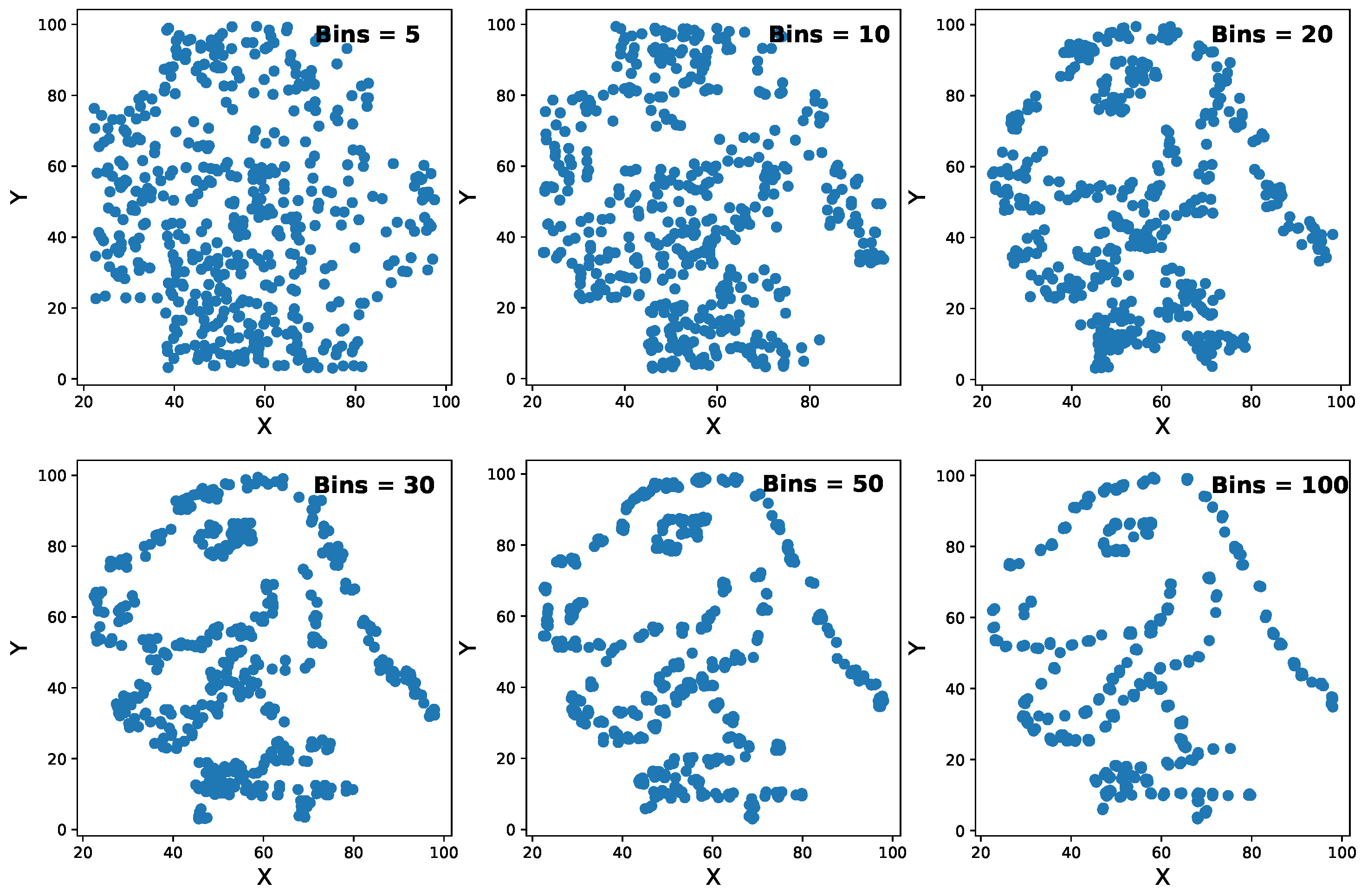
where $I_{\{·\}}$ is the indicator function. Note that $R\left(B_s\right)$ can be seen as a natural estimator for $F_i\left(a_s\right)$, thus some desirable properties will be considered below. In the context of density estimation, an important parameter to consider is the bandwidth denoted by h, which represents the radius of each element in the partition, i.e., $h=(a_j-a_{j-1})/2$. It is worth noting that the number of partitions t in Equation (2) depends on the bandwidth parameter as follows: $t=(X_{\left[n\right]i}-X_{\left[1\right]i})/\left(2h\right)$. Some methods for computing the bandwidth h are discussed in greater detail in Wasserman ([37], pp. 134–135).

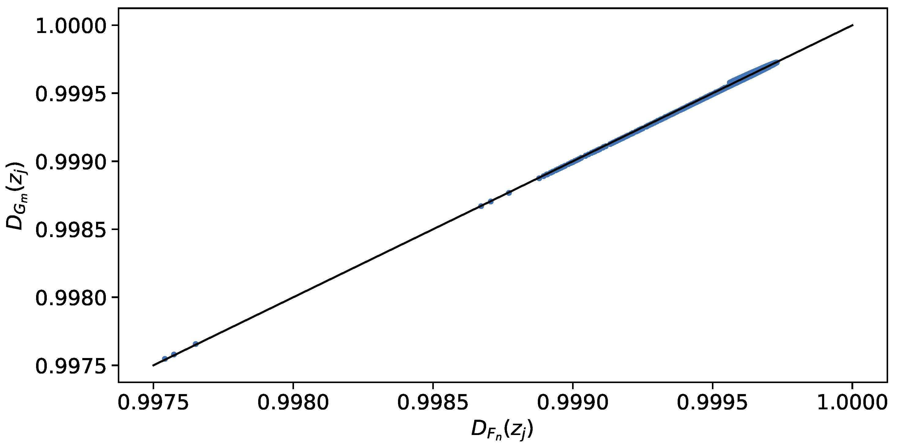
Proposition 1.

$R\left(B_s\right)$ is an unbiased estimator for $F_i\left(a_s\right)$

Proof. 

$$\begin{array}{cc}\hfill E\left[R\left(B_s\right)\right]& =E\left[\frac{1}{n}\sum _{j=1}^s\sum _{k=1}^n{I}_{\left\{X_{ki}\in B_j\right\}}\right]=\frac{1}{n}\sum _{j=1}^s\sum _{k=1}^{n}E\left[I_{\left\{X_{ki}\in B_j\right\}}\right]=\frac{1}{n}\sum _{j=1}^s\sum _{k=1}^{n}P\left(X_{ki}\in B_j\right)\hfill \\ \hfill & =\frac{1}{n}\sum _{j=1}^{s}n\left(F_i\left(a_j\right)-F_i\left(a_{j-1}\right)\right)=\sum _{j=1}^s\left(F_i\left(a_j\right)-F_i\left(a_{j-1}\right)\right)=-F_i\left(a_0\right)+F_i\left(a_s\right).\hfill \end{array}$$

However, $F_i\left(a_0\right)=P\left(X_i<X_{\left[1\right]i}\right)=0$; then, the proof is completed.    □

Previous results of Proposition 1 will be needed in the proof of the next proposition that states an asymptotic result.

Proposition 2.

$R\left(B_s\right)$ converges in quadratic mean to $F_i\left(a_s\right)$

Proof. 

$$\begin{array}{cc}\hfill V\left[R\left(B_s\right)\right]& =V\left[\frac{1}{n}\sum _{j=1}^s\sum _{k=1}^n{I}_{\left\{X_{ki}\in B_j\right\}}\right]=\frac{1}{n^2}\sum _{j=1}^s\sum _{k=1}^{n}V\left[I_{\left\{X_{ki}\in B_j\right\}}\right]\hfill \\ \hfill & =\frac{1}{n^2}\sum _{j=1}^s\sum _{k=1}^{n}P\left(X_{ki}\in B_j\right)\left[1-P\left(X_{ki}\in B_j\right)\right]\hfill \\ \hfill & =\frac{1}{n^2}\sum _{j=1}^{s}n\left(F_i\left(a_j\right)-F_i\left(a_{j-1}\right)\right)\left(1-F_i\left(a_j\right)+F_i\left(a_{j-1}\right)\right)\hfill \\ \hfill & =\frac{1}{n}\sum _{j=1}^s\left(F_i\left(a_j\right)-F_i\left(a_{j-1}\right)\right)\left(1-F_i\left(a_j\right)+F_i\left(a_{j-1}\right)\right)\le \frac{s}{n}.\hfill \end{array}$$

Therefore, $V\left[R\left(B_s\right)\right]$ converges to zero, and from Proposition 1, we have the desired conclusion.    □

It is recalled that, if one wants to generate univariate synthetic data from a known distribution $F_i\left(x\right)$, a simple form is using the inverse transform, i.e., one must generate a random variable Uniform in $[0,1]$ and then $X_i=F_i^{-1}\left(U\right)=inf\left\{X\right|F_i\left(X\right)\ge U\}$. However, if $F_i\left(x\right)$ is unknown but we have a sample $X_{1i},\cdots ,X_{ni}$ that comes from the distribution $F_i\left(x\right)$, the generation of synthetic data is more complicated. In this paper, considering the result obtained in Proposition 2, a methodology is proposed to generate univariate synthetic data but when one has a sample $X_{1i},\cdots ,X_{ni}$ that comes from the unknown distribution $F_i\left(x\right)$. Following the same idea considered in the inverse transform, one must generate a random variable U Uniform in $[0,1]$ and then calculate $min\left\{s\right|R\left(B_s\right)\ge U\}$ and so the synthetic data $\widehat{X}$ are generated by considering $\widehat{X}=a_{s-1}+(a_s-a_{s-1})U$.

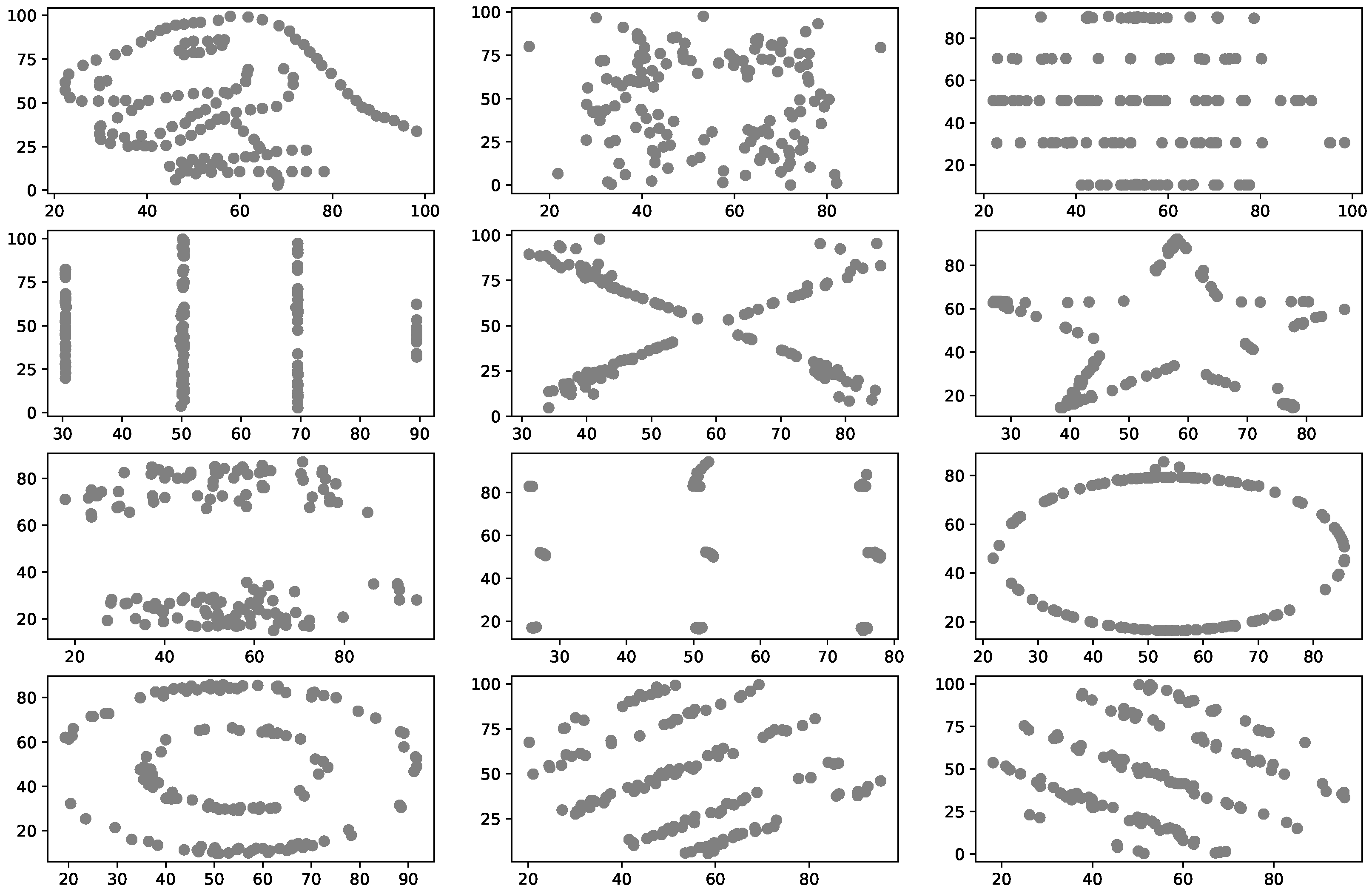
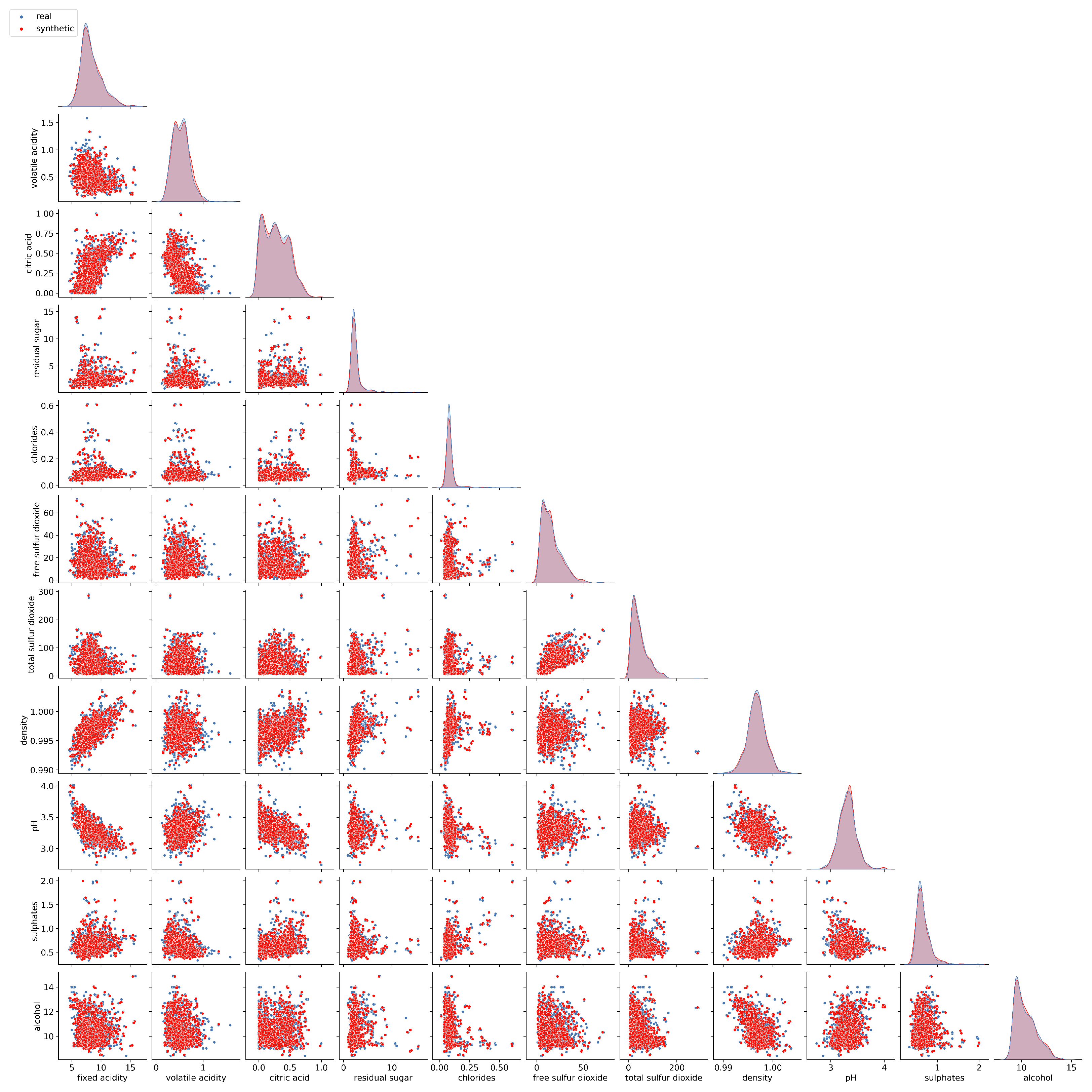
Example 1.

Let us simulate 300 data points from a standard Normal distribution. These 300 data points will be considered as an observed sample, i.e., raw data. Now, from those raw data, we will generate 1000 synthetic data points through the procedure introduced in this paper. The results on some relevant parameters can be seen in

Table 1. Population parameters of a standard normal distribution and their point estimates considering the raw data and synthetic data generated from those raw data.

Standard Normal	${\mathit{P}}_{25}$	Mean	Std	Median	${\mathit{P}}_{75}$
Theoretical Value	−0.6745	0	1	0	0.6745
Raw Data	−0.6504	−0.0023	0.9998	−0.0186	0.6368
Synthetic Data	−0.6425	−0.0028	1.0054	−0.0119	0.6502

.

We will generate 2000 collections of synthetic data, each comprising 1000 records and based on the same raw data that were previously considered. For each data set, the same values considered in Table 1 are calculated.

Table 2. Mean value and confidence intervals for the 2000 synthetic data collections.

Standard Normal	${\mathit{P}}_{25}$	Mean	Std	Median	${\mathit{P}}_{75}$
Mean Value	−0.6522	−0.0027	1.0026	−0.0135	0.6389
Confidence Interval	$[-0.6814-0.6207]$	$[-0.01210.0062]$	$\left[0.99351.0126\right]$	$[-0.04850.0220]$	$\left[0.60380.6706\right]$

displays the mean value and the $95\%$ confidence interval of each of those values.

Figure 2 shows the curve of theoretical distribution, the empirical distribution of raw data and the empirical distribution of synthetic data. Note that the raw data curve fits well to the theoretical distribution curve. This is not surprising because the raw data have been simulated from the theoretical distribution. However, the synthetic data generated from the raw data retain the same good-fit behavior. Note that the quality of the synthetic data depends on the quality of the observed raw data.

Example 2.

Let us now simulate 300 data points from an exponential distribution with mean 5. These 300 data points will be considered as an observed sample, i.e., raw data. From these raw data, we will generate 1000 synthetic data points. We followed the same steps as in the previous example.

Table 3. Population parameters of Exponential distribution and their point estimates considering the raw data and synthetic data generated from those raw data.

Exponential	${\mathit{P}}_{25}$	Mean	Std	Median	${\mathit{P}}_{75}$
Theoretical Value	1.4384	5	5	3.4657	6.9315
Raw Data	1.9618	5.1615	4.6496	3.8424	7.1929
Synthetic Data	1.7346	5.2074	4.5679	4.0704	7.5514

presents relevant parameters for these data.

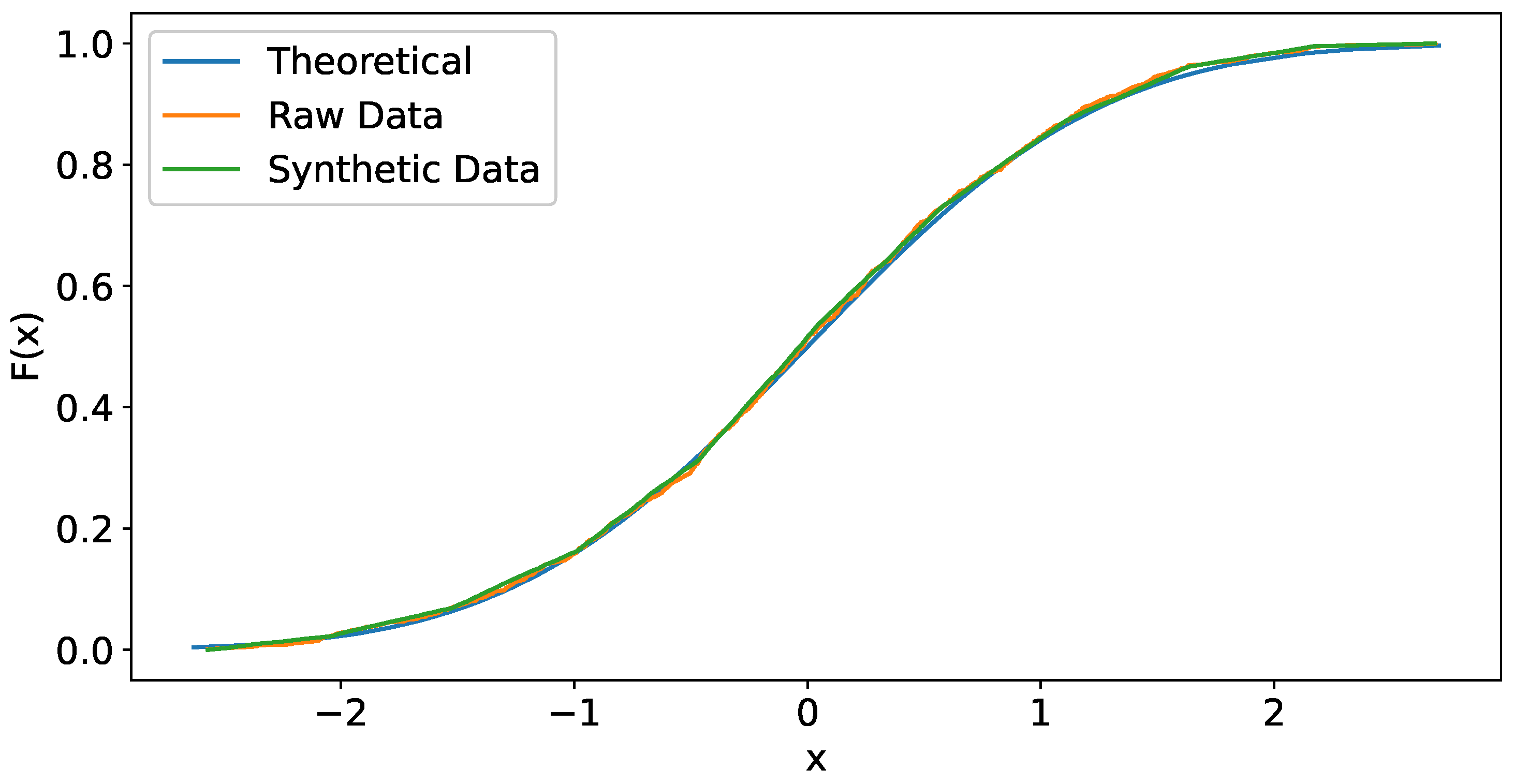
From the same raw data, we generate 2000 collections of synthetic data of same size 1000.

Table 4. Mean value and confidence intervals for the 2000 synthetic data collections.

Exponential	${\mathit{P}}_{25}$	Mean	Std	Median	${\mathit{P}}_{75}$
Mean Value	1.8482	5.2006	4.5643	3.9670	7.4234
Confidence Interval	$\left[1.71041.9759\right]$	$\left[5.14745.2500\right]$	$\left[4.51474.6143\right]$	$\left[3.81314.1276\right]$	$\left[7.16507.6706\right]$

displays the mean value and the 95% confidence interval of values considered in Table 3.

Figure 3 shows the curve of the theoretical distribution, the empirical distribution of raw data and the empirical distribution of synthetic data where a good fit can be observed.

Once the methodology to generate synthetic data from a univariate raw data sample has been designed, then we propose a technique to generate multivariate synthetic data from a multivariate data sample that comes from a random vector $\mathcal{X}=[X_1,\dots ,X_p]$ with multivariate distribution F, with $F_i$ being the marginal distribution of the random variable $X_i$.

Let $\mathbf{X}$ be a ${\mathbb{R}}^{n\times p}$ a matrix of the real data that comes from the random vector $\mathcal{X}$

$$\mathbf{X}=\left(\begin{array}{ccccc}{X}_{11}& ·& ·& ·& X_{1p}\\ ·& ·& ·& ·& ·\\ ·& ·& ·& ·& ·\\ ·& ·& ·& ·& ·\\ X_{n1}& ·& ·& ·& X_{np}\end{array}\right)$$

(3)

$\mathbf{X}$ is a raw data multivariate sample; one could think that, for generating synthetic data from $\mathbf{X}$, it is enough to generate, for each variable $X_i,i=1,\cdots ,p$, univariate synthetic data through the method introduced above, but the procedure is more complex because one must consider the dependence structure among marginal variables $X_i$. This dependence structure must be studied using a special dependence functions called copulas. We consider Nelsen [35] as the foremost general reference for an in-depth examination of copula theory.

A copula is a multivariate distribution function defined on ${[0,1]}^p$, where each of the p marginal distributions is a uniform distribution in $[0,1]$. According to Sklar’s theorem [17], any multivariate distribution function can be written in terms of the marginal distributions and a copula C, i.e., given a p-dimensional random vector $\mathcal{X}=[X_1,\dots ,X_p]$ with a multivariate distribution F, then

$$\begin{array}{c}\hfill F(x_1,\dots ,x_p)=P(X_1\le x_1,\dots ,X_p\le x_p)=C(F_1\left(x_1\right),\dots ,F_p\left(x_p\right)).\end{array}$$

Sklar’s theorem also states that the copula C is unique if the marginals $F_i\left(x_i\right)$ are continuous. The copula C contains the information on the dependence structure among the marginal random variables of $\mathcal{X}=[X_1,\dots ,X_p]$, and this dependence structure is an important aspect that must be considered when synthetic data are generated from the multivariate sample stated in the matrix of the real data $\mathbf{X}$ that comes from the random vector $\mathcal{X}$. From Equation (1), $F_i\left(X_i\right)\sim \mathrm{uniform}[0,1]$, thus the random vector

$$\begin{array}{c}\hfill [U_1,\dots ,U_p]=[F_1\left(X_1\right),\dots ,F_p\left(X_p\right)]\end{array}$$

(4)

has uniform marginals in $[0,1]$. Since each of $F_i$ is a non decreasing function, then the random vectors $[U_1,\dots ,U_p]$ and $[X_1,\dots ,X_p]=[F_1^{-1}\left(U_1\right),\dots ,F_p^{-1}\left(U_p\right)]$ have the same copula because the copula is invariant under non-decreasing transformations of the marginal random variables. Therefore, if there is a procedure to generate, from a known copula C, observations of the random vector $[U_1,\dots ,U_p]$, then a sample from $[X_1,\dots ,X_p]$ can be obtained as $[F_1^{-1}\left(U_1\right),\dots ,F_p^{-1}\left(U_p\right)]$; here, the marginal distributions also must be known. However, when neither the copula C nor the marginal distributions $F_i$ are known, only a real data multivariate sample as $\mathbf{X}$ is known, the previous procedure can not be implemented. Therefore, we introduce a new method for the generation of a new multivariate sample just knowing the multivariate sample stated in the matrix of the real data $\mathbf{X}$:

Define

$$\begin{array}{c}\hfill {\widehat{U}}_{ji}=\frac{1}{n}\sum _{k=1}^n{I}_{\{X_{ki}\le X_{ji}\}},\forall i\in \{1,\cdots ,p\},\end{array}$$

(5)

where $I_{\{·\}}$ is the indicator function. Note that ${\widehat{U}}_{ji}$ is the empirical distribution of observed value $X_{ji}$ with respect to the observed sample just of the i-th variable. Therefore, following Equation (4), the following matrix,

$$\widehat{U}=\left(\begin{array}{ccccc}{\widehat{U}}_{11}& ·& ·& ·& {\widehat{U}}_{1p}\\ ·& ·& ·& ·& ·\\ ·& ·& ·& ·& ·\\ ·& ·& ·& ·& ·\\ {\widehat{U}}_{n1}& ·& ·& ·& {\widehat{U}}_{np},\end{array}\right)$$

(6)

is the p-dimensional support of the empirical copula estimated from multivariate sample $\mathbf{X}$, where the columns of $\widehat{U}$ are samples that come from random vector $[U_1,\dots ,U_p]$ considered in Equation (4) and thus those samples come from the same copula C, which is the same copula that has the random vector $\mathcal{X}=[X_1,\dots ,X_p]$, from which comes the raw data multivariate sample stated in matrix $\mathbf{X}$. Since the copula C is unknown, the new procedure introduced just considers the p-dimensional support of the empirical copula estimated from multivariate sample $\mathbf{X}$ as follows.

For the i-th column in $\mathbf{X}$, consider a partition of the interval $[X_{\left[1\right]i},X_{\left[n\right]i}]$ as $X_{\left[1\right]i}=a_{0i}<a_{1i}<\cdots <a_{t_{i}i}=X_{\left[n\right]i}$. Define $B_{si}$ as:

$$\begin{array}{c}\hfill B_{si}=\left\{\begin{array}{cc}[a_{(s-1)i},a_{si}]\hfill & \mathrm{if}s=1\\ \\ (a_{(s-1)i},a_{si}]\hfill & \mathrm{otherwise}\end{array}\right.\end{array}$$

$$\begin{array}{c}\hfill R\left(B_{si}\right)=\frac{1}{n}\sum _{j=1}^s\sum _{k=1}^n{I}_{\left\{X_{ki}\in B_{ji}\right\}},\forall s\in \{1,\cdots ,t_i\}.\end{array}$$

(7)

Note that $R\left(B_{si}\right)$ can be seen as a natural estimator for $F_i\left(a_{si}\right)$, and from Proposition 1, the vector $\left[R\left(B_{s1}\right),\dots ,R\left(B_{sp}\right)\right]$ is an unbiased estimator of the vector $\left[F_i\left(a_{s1}\right),\dots ,F_i\left(a_{sp}\right)\right]$.

Let d be a value generated from a discrete uniform distribution in $\{1,\dots ,n\}$. Since the copula C is unknown, we use the the p-dimensional support of the empirical copula by selecting the d-th row of $\widehat{U}$. Following the same idea considered in the inverse transform, one must generate a random variable U Uniform in $[0,1]$; then, for each $i\in \{1,\dots ,p\}$, calculate $min\left\{s\right|R\left(B_{si}\right)\ge {\widehat{U}}_{di}\}$ and so a multivariate synthetic piece of data $[{\widehat{X}}_1,\dots ,{\widehat{X}}_p]$, with the same statistics structure as marginals and dependence of those data stated in the matrix of the real data $\mathbf{X}$, can be generated by considering ${\widehat{X}}_i=a_{(s-1)i}+(a_{si}-a_{(s-1)i})U$ for all $i\in \{1,\dots ,p\}$.

Algorithm 1 synthesizes the set of steps formalized above. The described procedure is implemented in the GitHub repository https://github.com/jurest82/SyntheticDataCopulas (accessed on 31 January 2023) using Python3.

Algorithm 1: Synthetic Data Generation Algorithm

To understand how the performance of the algorithm scales related to the size of the parameters N, n, p and T, we analyze the complexity of Algorithm 1. First, computing the empirical distribution function along the frequency tables for all variables is $\mathcal{O}\left(pnlog\right(n\left)\right)$ time. In addition, the worst time of evaluating an empirical distribution function is $\mathcal{O}\left(log\right(n\left)\right)$, and repeated to every element in matrix $\mathbf{X}$ is then $\mathcal{O}\left(pnlog\right(n\left)\right)$. Let $t=ma{x}_{i\in \{1,\dots ,p\}}T\left[i\right]$, and the creation of a datum is bounded by $\mathcal{O}\left(plog\right(t\left)\right)$ time. Therefore, the generation of a sample of size N is $\mathcal{O}\left(Nplog\right(t\left)\right)$ time. Thus, the worst time complexity of the Synthetic Data Generation Algorithm is $\mathcal{O}\left(pnlog\right(n)+Nplog(t\left)\right)$ and since t is bounded by n, the expression can be simplified to $\mathcal{O}\left(max\right(N,n\left)plog\right(n\left)\right)$.

2.2. Experiments

To illustrate the goodness of the method, several experiments were carried out. The first group of experiments corresponds to generating SD from realizations of RD following a distribution $\mathcal{F}$. The generated data and the real data are compared using scatter plots since they are presented only as an illustration. To generate the data $x^{\left(1\right)},\dots ,x^{\left(n\right)}\in \mathbb{R}{}^p,\mathrm{p}=2,3$, are sampled from $\mathcal{F}$. The patterns with which these real data are obtained are identified as (a) cubic function, (b) two-dimensions spiral, (c) Batman logo, (d) petals and (e) three-dimensions spiral. These cases were chosen since, in general, they present patterns with complex geometries, which allows us to demonstrate that, even in complex cases, the data generation method works correctly.

The second group of experiments corresponds to the generation of data from the real data set known as Wine Quality Data Set, which corresponds to data on the physicochemical properties of red wine and is taken from [38]. For this experiment, the RD are compared with the synthetic ones using scatter plots, probability density plots and with the multivariate homogeneity test explained in Section 2.3. This case is presented to show that the method maintains good results even in high-dimensional data sets.

2.3. Homogeneity Test

Liu et al. [36] present a method to determine if two multivariate distributions come from the same population. The method is based on data depth plots of their samples. In this article, we use the above method to show that the samples generated by the data augmentation algorithm follow the same multivariate distribution as the RD.

Liu et al. [36] propose the DD-plot, which corresponds to a plot of the combined sample depth under the two corresponding empirical distributions. If the distributions are identical, i.e., come from the same population, then the depth plot is a segment of a straight line joining the points $(0,0)$ and $(1,1)$ in ${\mathbb{R}}^2$. If there is any deviation of said graph from the straight line, then it is a sign that the distributions are not identical.

Formally, let $D(·)$ be an affine invariant depth and let F and G be two distributions on ${\mathbb{R}}^p$, and $DD(F,G)$ is defined as follows:

$$DD(F,G)=\left\{(D_F\left(z\right),D_G\left(z\right))\mathrm{for}\mathrm{all}z\in {\mathbb{R}}^p\right\}$$

If the distributions are unknown, then an empirical version of the DD-plot must be used; for example, if F and G are a set of observations $\left\{X_1,X_2,\dots ,X_n\right\}(\equiv \mathbf{X})$, $\left\{Y_1,Y_2,\dots ,Y_m\right\}(\equiv \mathbf{Y})$, respectively, the DD-plot is defined as follows:

$$DD(F_n,G_m)=\left\{(D_{F_n}\left(z_j\right),D_{G_m}\left(z_j\right)),z_j\in \left\{\mathbf{X}\cup \mathbf{Y}\right\}\right\}$$

(8)

Since, in practice, we do not know the multivariate distribution, then the expression given by Equation (8) was used in our experiments. In the particular case of this investigation, the depth measurement is given by a normalization of the metric induced by the p norm:

$$\begin{array}{c}\hfill D_{F_n}\left(z_j\right)=1-\frac{{\sum }_{i=1}^n{∥X_i-z_j∥}_p}{{\sum }_{j=1}^{n+m}{\sum }_{i=1}^n{∥X_i-z_j∥}_p},\forall z_j\in \left\{\mathbf{X}\cup \mathbf{Y}\right\}\\ \hfill D_{G_m}\left(z_j\right)=1-\frac{{\sum }_{i=1}^m{∥Y_i-z_j∥}_p}{{\sum }_{j=1}^{n+m}{\sum }_{i=1}^m{∥Y_i-z_j∥}_p},\forall z_j\in \left\{\mathbf{X}\cup \mathbf{Y}\right\}.\end{array}$$

(9)

In particular, we use $p=2$ in Equation (9), that is, the Euclidean norm.

To prove by statistical inference that the points $(D_{F_n}\left(z_j\right),D_{G_m}\left(z_j\right))$ lie on the straight line joining the points $(0,0)$ and $(1,1)$, it is enough to show that the tuples follow a linear relationship and that, if a simple linear regression is fitted, then the confidence interval of the intercept ${\beta }_0$ contains zero, the confidence interval of the slope ${\beta }_1$ contains one, and the coefficient of determination $R^2$ is very close to one. We follow the approach described to show that the generated data come from the same distribution as the original data; for this, we estimate bootstrap confidence intervals of 95% by the percentile method, as explained in ([37], pp. 27–39).

2.4. Sensitivity Analysis

Section 2.1 discusses an essential parameter of the method known as the number of partitions represented by t. This parameter determines the number of bins or partitions in a frequency table used to generate SD. In this section, we explain the simulation analysis carried out to study the effect of t on the quality of the synthetic data.

We run a simulation using the raw data from the first scatterplot in Figure 1. We generate new data with fixed t and the same value for both dimensions of the plot. We repeated this process for six different values of $t=5,10,20,30,50,$ and 100. SD was visually compared using scatterplots.

3. Results and Analysis

In this section, the obtained results from the experiments explained in Section 2.2 are analyzed. Figure 4 presents five pairs of scatter plots of the following patterns: (a) cubic function, (b) two-dimensions spiral, (c) Batman logo, (d) petals, and (e) three-dimensions spiral. Blue dots represent real data, while red dots correspond to synthetically generated data. As can be seen, the plots of the SD are very similar to the plots of the real observations. No matter what geometry needs to be replicated, the data augmentation method can learn the underlying dependency relationships and probability distributions. This first group of experiments allows us to demonstrate graphically and simply the goodness of the synthesis method.

Regarding the wine quality data obtained from [38], we must observe the respective scatter and probability density plots depicted in Figure 5.

Figure 5 shows that the geometric shape of the probability distributions are identical, that is, the SD generation method respects the marginal distributions of each variable. Moreover, when analyzing the scatter plots, it is observed that the bivariate dependency relationships are also respected by the proposed method since the geometric shape and the scale are identical to those of the RD. In practice, these facts indicate that synthetic data are similar to real data in univariate and bivariate parameters. Univariate parameters, such as mean, median, standard deviation, interquartile range, kurtosis, and skewness, are identical in SD and RD. Bivariate parameters, such as covariance, Pearson’s correlation, and Spearman’s correlation, are identical for both data sets. This indicates that the SD accurately captures the relationships and patterns present in the RD.

However, as explained before, to conclude that the joint distribution of the real and synthetic data are equivalent, it is not enough to look at the marginal distributions and the bivariate dependency relationships. A homogeneity test needs to be used to conclude whether two multivariate data sets have the same joint distribution.

Figure 6 corresponds to the DD-plot explained in Section 2.3, where $F_n$ corresponds to the original data and $G_m$ to the generated samples. It should be noted that the depth values form a straight line that, fitting a simple linear regression model, yields a confidence interval for $R^2$ of $[0.9922,0.9999]$, a confidence interval for intercept ${\beta }_0$ of $[-0.0957,0.0618]$ and a confidence interval for the slope ${\beta }_1$ of $[0.9069,1.1087]$. Therefore, the homogeneity test confirms that the generated samples come from the same multivariate distribution as the original data, since the line they form is a segment of the straight line that joins the points $(0,0)$ and $(1,1)$ in ${\mathbb{R}}^2$ because $R^2$ is very close to one, and it cannot be rejected that ${\beta }_0$ is zero and that ${\beta }_1$ is one with a confidence level of 95%.

In Section 2, we mentioned that the number of bins used in the frequency tables can significantly affect the result of Algorithm 1. To illustrate this, Figure 7 shows six data sets generated from the raw data contained in the first scatterplot of Figure 1. Each of these data sets was created using a different number of partitions.

As shown in Figure 7, the number of bins used has a noticeable effect on the similarity between synthetic and real data sets. Specifically, we find that increasing the number of bins results in SD, which more closely reflects the dependency structure of the raw data. Conversely, using a low number of bins fails to capture this structure accurately. However, a very high number of partitions can produce synthetic data with less variability.

The question of how to select the optimal number of partitions for a frequency table, histogram, or density estimate is outside the scope of this research. For more in-depth analysis on this topic, interested readers may refer to works such as Hollander et al. ([39], pp. 609–628), Silverman [40], and Wasserman ([37], pp. 125–142), among others.

A notable result of the sensitivity analysis is that the six data sets shown in Figure 7 are marginally equal to each other. To illustrate this point, we present

Table 5. Summary statistics for selected plots of Figure 7.

	Variable	Mean	Std	${\mathit{P}}_{25}$	${\mathit{P}}_{50}$	${\mathit{P}}_{75}$
bins = 5	X	54.9	17.9	40.9	53.9	66.8
	Y	46.3	26.9	24.3	44.7	65.8
bins = 100	X	54.9	16.6	45.5	52.9	64.5
	Y	46.6	28.0	23.5	41.5	71.3

, which contains summary statistics for the cases where $t=5$ and $t=100$. While these statistics are fairly similar between partitions, we note that the method does not capture the multivariate dependency structure effectively when $t=5$, but it does when $t=100$. Therefore, we conclude that increasing the value of t can improve the performance of the method.

4. Conclusions

This article presents a novel nonparametric method for generating synthetic data using copulas. Said method is easy to use, implement and interpret, but more importantly, synthetic data generated by the method maintain identical marginal and joint distributions and the same dependency relationships as real data. Preserving the statistical properties of raw data are a fundamental property of the algorithm that enhances confidence in using synthetic data for practical applications. This is useful in realistic scenarios such as class balancing in machine learning algorithms, protecting sensitive information in financial and healthcare domains, and more. The aforementioned fact was illustrated with an example in which a multivariate homogeneity test was used, something that is not usually found in the scientific literature on data augmentation. The proposed method is promising, and it will be of interest for future research to use it to increase the performance of machine learning models and adapt it to perform multivariate imputation, among others. Furthermore, determining the optimal way to select the unique hyperparameter of the model, i.e., the number of bins, is relevant for forthcoming studies.

The proposed algorithm has two crucial limitations. First, it only works with tabular data, as it has not been extended to unstructured data such as text, images or audio, which limits its applicability to data augmentation problems in deep learning applications. Expanding the algorithm’s compatibility with unstructured data will be a crucial advance in future research. Secondly, the formulation does not account for categorical variables. As a result, the method cannot generate data from a tabular dataset that includes this variable type.