A Freehand 3D Ultrasound Reconstruction Method Based on Deep Learning

Abstract

In the medical field, 3D ultrasound reconstruction can visualize the internal structure of patients, which is very important for doctors to carry out correct analyses and diagnoses. Furthermore, medical 3D ultrasound images have been widely used in clinical disease diagnosis because they can more intuitively display the characteristics and spatial location information of the target. The traditional way to obtain 3D ultrasonic images is to use a 3D ultrasonic probe directly. Although freehand 3D ultrasound reconstruction is still in the research stage, a lot of research has recently been conducted on the freehand ultrasound reconstruction method based on wireless ultrasonic probe. In this paper, a wireless linear array probe is used to build a freehand acousto-optic positioning 3D ultrasonic imaging system. B-scan is considered the brightness scan. It is used for producing a 2D cross-section of the eye and its orbit. This system is used to collect and construct multiple 2D B-scans datasets for experiments. According to the experimental results, a freehand 3D ultrasonic reconstruction method based on depth learning is proposed, which is called sequence prediction reconstruction based on acoustic optical localization (SPRAO). SPRAO is an ultrasound reconstruction system which cannot be put into medical clinical use now. Compared with 3D reconstruction using a 3D ultrasound probe, SPRAO not only has a controllable scanning area, but also has a low cost. SPRAO solves some of the problems in the existing algorithms. Firstly, a 60 frames per second (FPS) B-scan sequence can be synthesized using a 12 FPS wireless ultrasonic probe through 2–3 acquisitions. It not only effectively reduces the requirement for the output frame rate of the ultrasonic probe, but also increases the moving speed of the wireless probe. Secondly, SPRAO analyzes the B-scans through speckle decorrelation to calibrate the acousto-optic auxiliary positioning information, while other algorithms have no solution to the cumulative error of the external auxiliary positioning device. Finally, long short-term memory (LSTM) is used to predict the spatial position and attitude of B-scans, and the calculation of pose deviation and speckle decorrelation is integrated into a 3D convolutional neural network (3DCNN). Prepare for real-time 3D reconstruction under the premise of accurate spatial pose of B-scans. At the end of this paper, SPRAO is compared with linear motion, IMU, speckle decorrelation, CNN and other methods. From the experimental results, it can be observed that the spatial pose deviation of B-scans output using SPRAO is the best of these methods.

1. Introduction

Medical imaging is important for physicians to visualize the inner anatomy of patients for diagnosis and analysis. Compared with computer tomography (CT) and the magnetic resonance imaging (MRI), ultrasonic imaging has the advantages of being used in real time, portability, low cost and causing no harm to the patient. Physicians use the ultrasonic probe to conveniently move the subject’s skin to examine the region of interest (ROI). The ultrasound probe outputs 2D ultrasound images for the physician to view. However, there are many limitations in relying on 2D ultrasound images during ultrasound scanning. Using 3D ultrasound imaging can clearly display the 3D contour of the measured object and the slice map in multiple directions. Therefore, physicians can work without too much mental labor. Three-dimensional ultrasound images are obtained via 3D reconstruction of a series of 2D ultrasound images. Before 3D reconstruction, there are several methods for data acquisition, including 2D array, mechanical, tracked freehand, and untracked freehand [1,2,3,4]. Because the acquisition method of a freehand linear array probe can not only control the size of the scanning area but is also low-cost, this method is particularly suitable for popularization [5].

At present, there are three main freehand 3D imaging methods: (1) fixing a linear array ultrasonic probe on a robot arm for scanning [6,7,8,9,10,11]; (2) use of an ultrasonic probe with external sensors for scanning [12,13,14,15]; and (3) use of a sensorless ultrasonic probe for scanning. In contrast, a 2D array scanning system is very expensive and difficult to develop in hardware and software [16]. Therefore, the application of a cheaper linear array has attracted attention. A linear array ultrasound probe is also known as the 2D ultrasound probe.

Using a robot arm for scanning is similar to using mechanical positioning tracking, such as linear tracking systems [8,9,10,11]. Chung used eight high-performance digital cameras to track a small rigid body mounted on an ultrasonic probe to realize optical motion tracking [12]. A Bayesian based nonlocal method was used for accurate volume reconstruction of irregular interval B-scan freehand 3D ultrasound imaging. This method uses gamma distribution instead of traditional Rayleigh distribution to achieve better suppression of speckle noise [17]. A game controller position tracker has also been used to design and manufacture a low-cost 3D ultrasound system based on standard 2D ultrasound. A Playstation’s mobile location tracking not only provides a low-cost alternative, but is also a portable device [18]. Gao verified the feasibility of using wireless communication technology and an image-based motion tracking method to realize 3D ultrasound imaging.

Neural networks are used to track the B-scan action to complete 3D reconstruction [19] and learn the speckle elimination correlation curve [20,21,22,23]. Cui Yang [24] uses a six degree of freedom robotic arm taking the role of the physician. A full convolutional network (fuse U-NET) based on a depth sensor and depth image is proposed to realize the automatic recognition of the human spinal region and pre-planning of the scanning path. Prevost R uses statistical learning and a convolutional neural network for modelling, which verifies the feasibility of predicting the motion of the ultrasound probe through the ultrasound image itself [25]. Guo proposed a deep-level context analysis learning network (DCL-NET), which uses the feature relationship between ultrasonic image frames to perform 3D reconstruction without sensors [26]. In another article, an improved adaptive strategy is proposed, which generates invariant features by minimizing the difference of image features of samples so that the deep learning algorithm can adapt to the data collected by different sensors [27]. Luo M [28] proposed an online learning framework that can deal with complex sequences. An evaluation was carried out on self-scanned datasets, and good results were obtained [29,30]. Later, the method based on deep learning was extended, and measurement data from an inertial measurement unit (IMU) were added to the process [31]. It can not only reconstruct the volume from the cross-sectional sequence, but also reconstruct the context information from the test data themselves, thus improving the perception ability of the neural network model. Su proposed a 3D-CNN model that can simultaneously extract features from space and time through 3D convolution. This model can capture motion information of multiple adjacent frames [32]. Su [33] performed a detailed analysis and comparison on different models of sequence extraction and candidate sequence classification, including U-NET [34,35] + CNN-LSTM, CNN-LSTM [36,37,38], V-NET, R-CNN+3D-CNN [39,40], etc. Xie proposed a convolutional neural network for 3D reconstruction by adding a pyramid distortion layer to fuse ultrasonic image and optical flow characteristics [41].

Generally speaking, the first method mainly relies on automation instead of manual operation. The advantages are high imaging accuracy and strong stability; however, the equipment is large in size and high in cost. Controlling the close coupling between robot probe and human skin is a very important challenge. In the second method, the data collected are generally a combination of the 2D ultrasound image sequence and its relative spatial information, as provided by an external auxiliary positioning device. The advantages of a freehand scanning system without using a position sensor are the low cost and scanning flexibility. However, the 2D ultrasound frames acquired by the system are usually irregular intervals between images, which may cause undesirable artifacts in the reconstruction results. Therefore, it is necessary to research and develop reconstruction methods or algorithms, for example, linear motion, IMU, speckle decorrelation, CNN, to optimize the reconstruction results. The optical positioning sensor has high stability, strong anti-interference ability and high positioning accuracy; however, it cannot solve the occlusion problem in the process of freehand scanning.

In this paper, a freehand 3D ultrasonic reconstruction method based on deep learning is proposed. This method is named sequence prediction reconstruction based on acousto-optic localization (SPRAO). The research architecture diagram of SPRAO is shown in Figure 1. The advantages and disadvantages of using and not using SPRAO in freehand 3D reconstruction are compared. The organization of this article is designed according to the innovation of SPRAO in Figure 1. The implementation process of SPRAO is as follows:

(1)

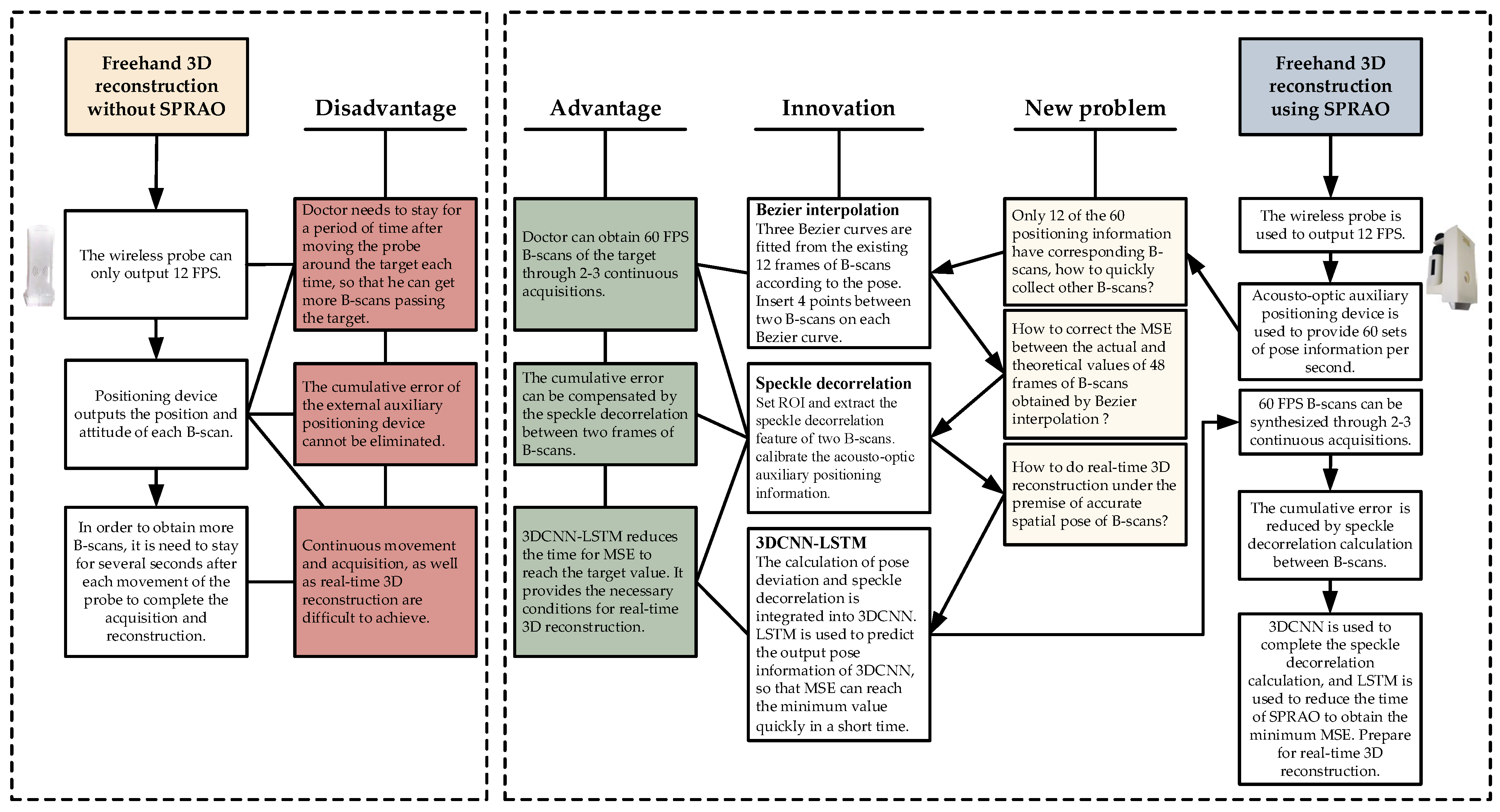
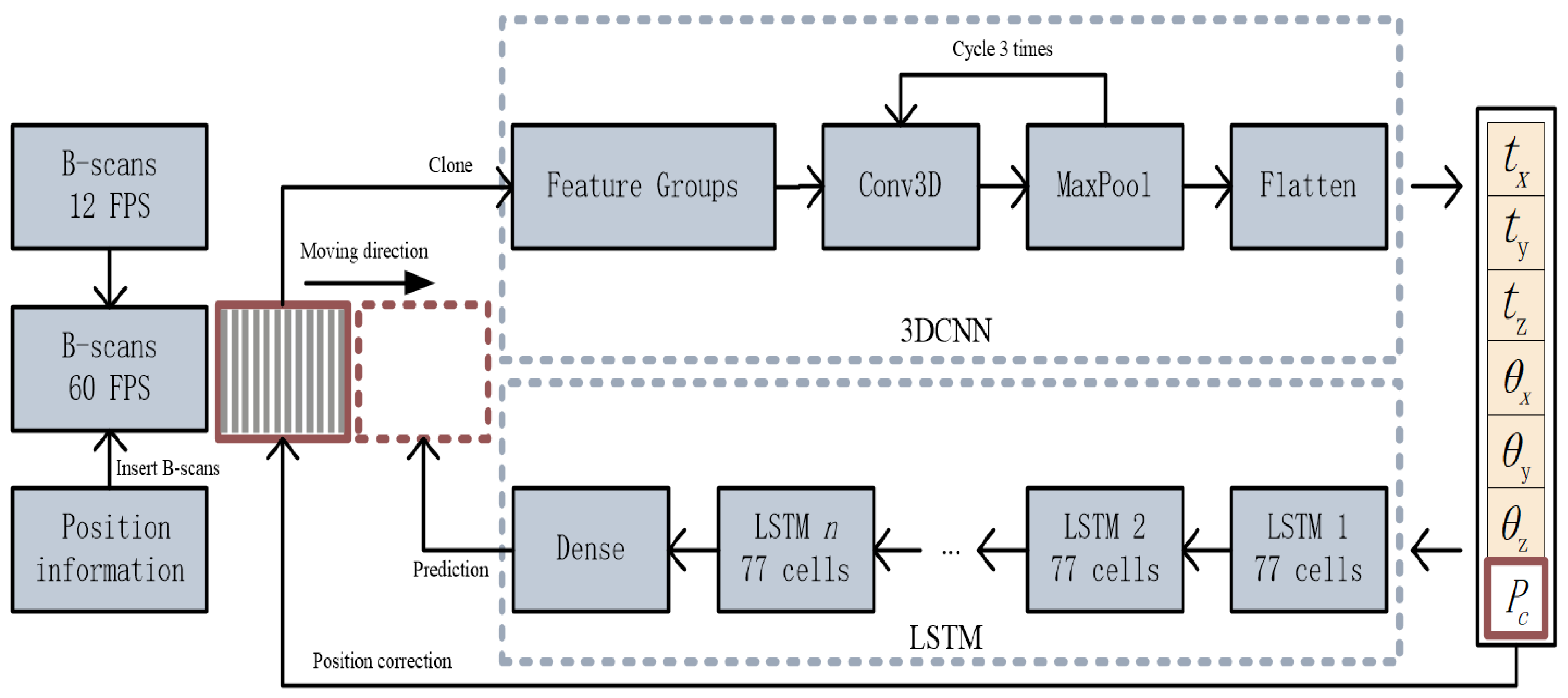
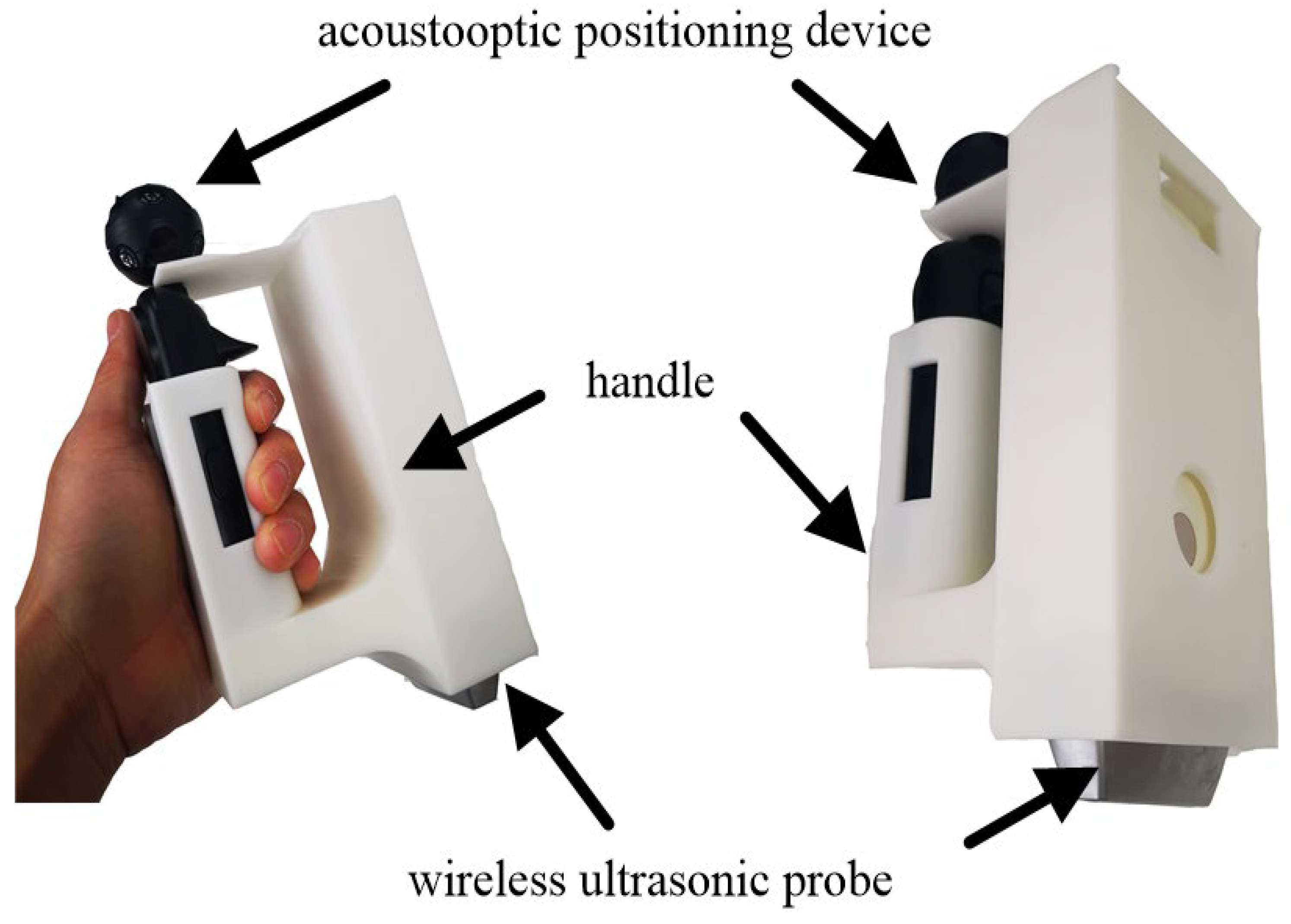
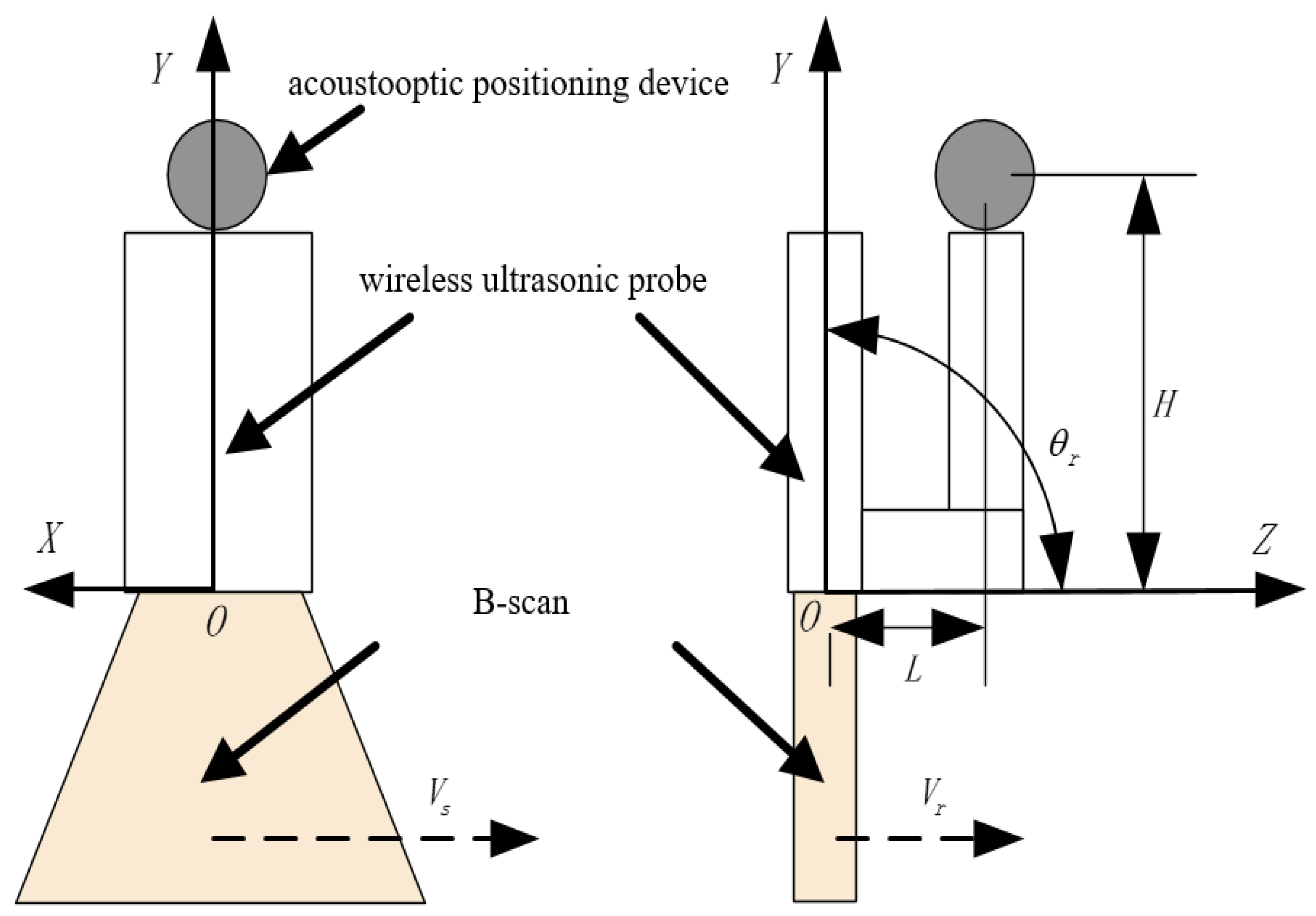
An acousto-optic positioning handheld device based on linear array wireless ultrasonic probe is designed and fabricated. The wireless probe outputs 12FPS B-scans raw data. Acousto-optic auxiliary positioning device is used to provide 60 sets of pose information per second. If each group of pose information output can directly correspond to a frame of B-scan, this is not a challenging problem. However, the real situation is that it is impossible to continuously collect with a handheld probe. For example, when we move continuously for 1 s at a speed of 1 cm/s, we can only obtain 12 FPS B-scans within a distance of 1 cm, although we obtain 60 sets of pose data. Among them, there are 48 groups of posture information without corresponding B-scans. Therefore, in this paper, the algorithm and training model are designed to make the probe collect the least number of times in the range of 1 cm, and finally synthesize 60 FPS B-scans within 1 cm. A 3D ultrasound imaging system can not only collect data, but it can also provide support for the SPRAO algorithm in this paper. It can be seen from Figure 1 that the innovation and advantages of the SPRAO algorithm require the spatial pose information output by the acousto-optic positioning device.

(2)

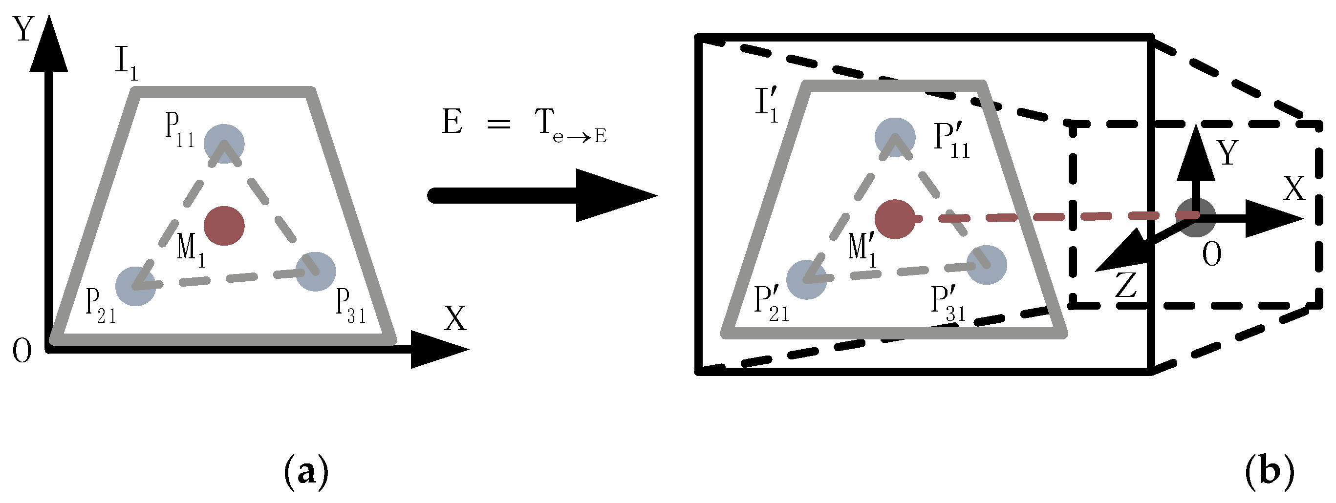
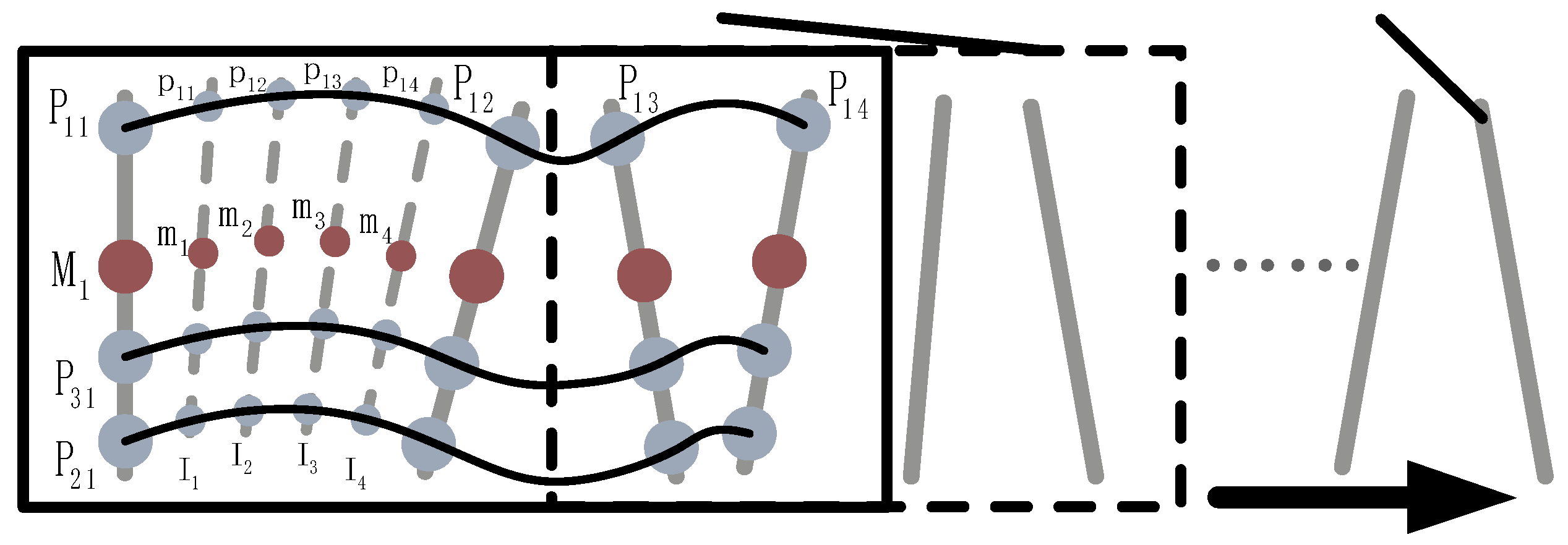
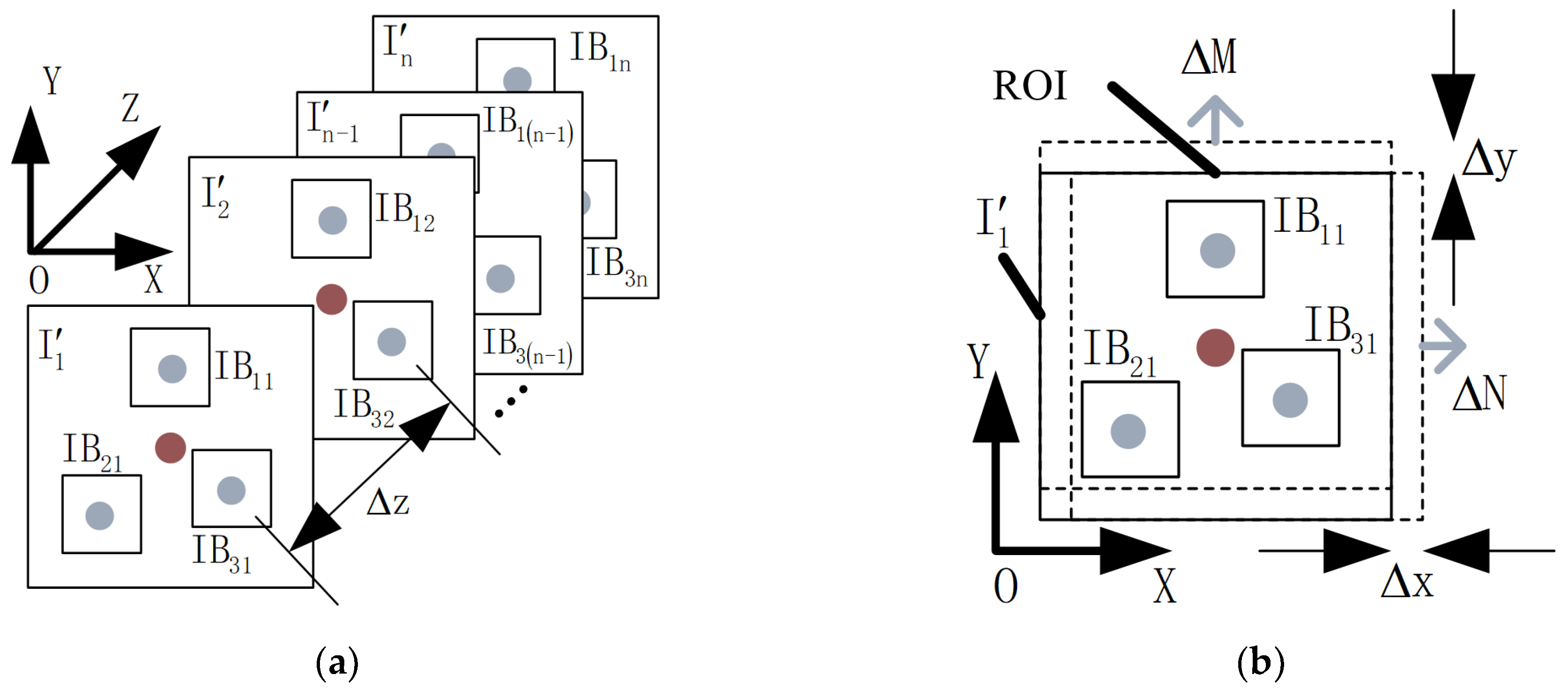
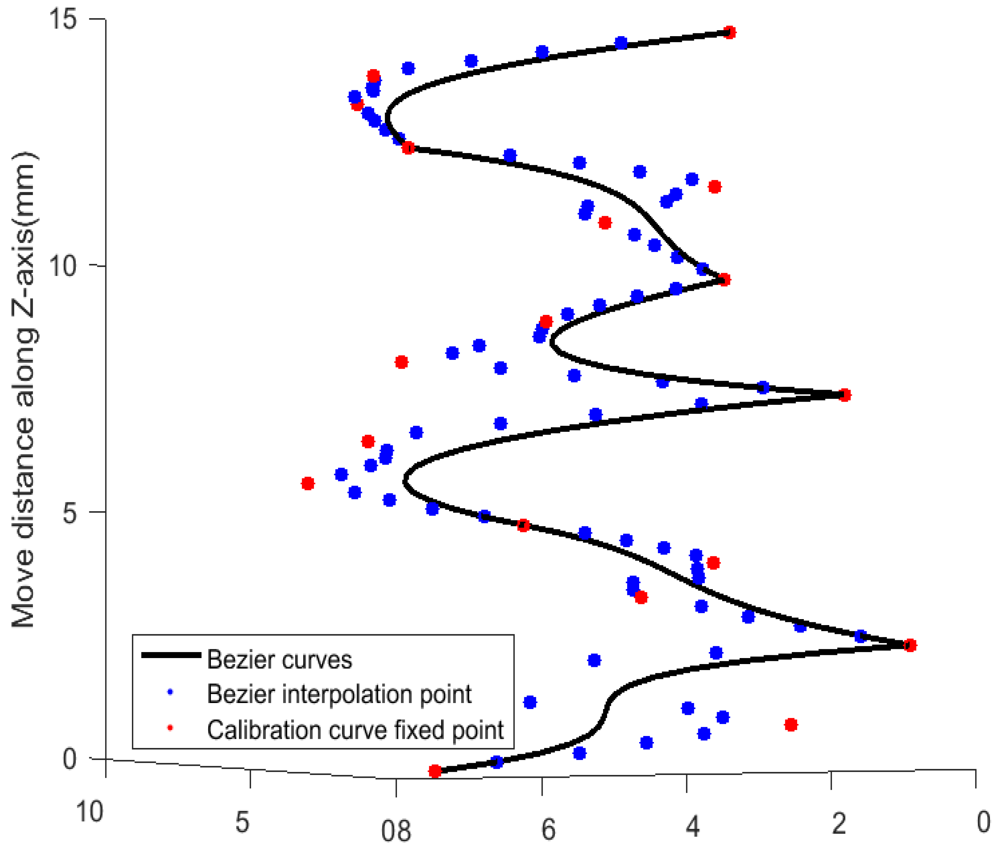
Because the surface of the measured target will change due to the extrusion of the probe, the position of the target will also change when the probe is collected back and forth. The effect of 3D reconstruction using pose information directly is not good; thus, curve fitting and speckle decorrelation are needed for position correction. The probe can only obtain 12 frames of B-scans after the first acquisition. We need to insert another 48 frames of B-scans through subsequent acquisition. The spatial position of each frame of B-scans is actually determined by three points on different lines in the space; therefore, three Bezier curves are needed to provide three points for each plane. Three Bezier curves are fitted from the existing 12 frames of B-scans according to the pose. Four points are inserted between two B-scans on each Bezier curve. The original data is interpolated and synthesized on a Bezier curve. This not only ensures the frame rate of the B-scan sequences, but also reduces the requirement of ultrasonic probe output frame rate.

(3)

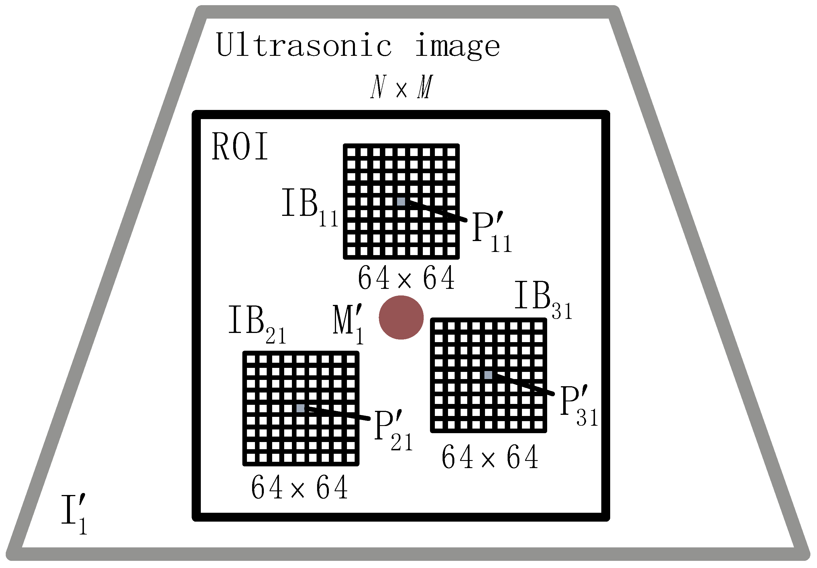
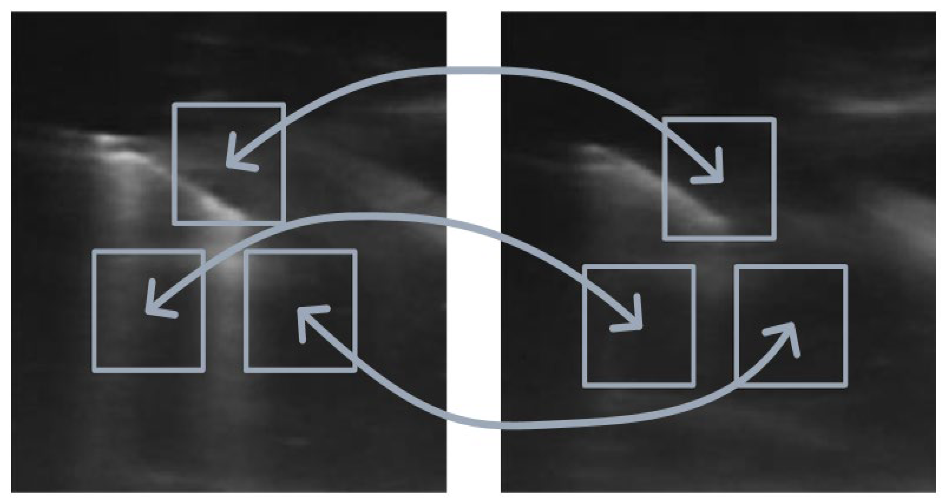
Set ROI and extract the speckle decorrelation feature of two B-scans. Calibrate the acousto-optic auxiliary positioning information. It should be noted that through the speckle decorrelation results of two frames of B-scans, the reduction is not the interpolation error but the change error caused by the extrusion of the probe. The mean square error (MSE) loss function is used to represent the difference between the calculation result and the real value. The correct MSE between the actual and theoretical values of 48 frames of B-scans is obtained through Bezier interpolation.

(4)

The calculation of pose deviation and speckle decorrelation is integrated into 3DCNN. LSTM is used to predict the output pose information of 3DCNN, so that MSE can reach the minimum value quickly in a short time. 3DCNN-LSTM extracts deep abstract features and establishes a model to predict the spatial pose of the ultrasonic probe. Finally, the 3D reconstruction of B-scans sequence is realized.

Compared with linear motion, IMU, speckle decorrelation or CNN, SPRAO can not only reduce the output frame rate requirement of the wireless probe, but also reduce the cumulative error of the positioning device via speckle decorrelation between two frames of B-scans. 3DCNN is used to complete the speckle decorrelation calculation. LSTM is used to reduce the time of SPRAO to obtain the minimum MSE, which is useful for real-time 3D reconstruction. The contributions of this paper are as follows:

• Bezier interpolation and Speckle decorrelation are applied to the data acquisition process of freehand 3D ultrasound reconstruction so that doctors can obtain 60 FPS B-scans of the target through 2–3 continuous acquisitions.
• By extracting the speckle decorrelation feature of two B-scans, the acousto-optic-assisted positioning information is compensated, and the cumulative error of the positioning device in the freehand 3D ultrasound reconstruction process is solved.
• The deep learning model 3DCNN-LSTM is used to implement the algorithm. The calculation of pose deviation and speckle decorrelation is integrated into 3DCNN. LSTM is used to predict the output pose information of 3DCNN so that MSE can reach the minimum value in a short time.

2. Materials and Methods

2.1. Bezier Interpolation

It has been mentioned in the Introduction section that because only 12 FPS B-scans can be obtained after the first acquisition of the probe, there are 48 sets of pose information without corresponding B-scans in the 60 sets of pose raw data per second. Another 48 frames of B-scans need to be inserted through the subsequent acquisition process. The spatial position of each frame of B-scans is actually determined by three points on different lines in the space; therefore, three Bezier curves are needed to provide three points for each plane. The degree of Bezier polynomial used in this paper is not large, and the Bezier curve is more in line with the moving trajectory of the handheld probe in space. Therefore, the data obtained via Bezier interpolation is used as the basis for the improvement of B-scans’ frame rate [42,43,44]. In reference [30], the frame rate of B-scan sequences used in the experiment is 35 FPS; however, it is difficult for a general wireless ultrasonic probe to have such a performance. For example, the frame rate of the wireless ultrasound probe used in this paper is only 12 FPS. In order to obtain a high frame rate in the B-scan sequence, it is necessary to fit several Bezier curves in the original B-scans sequence and calculate the coordinate position of the space insertion point on the Bezier curve.

The higher the order, the longer the construction time of the Bezier curve, and the higher the computational complexity of its interpolation. Therefore, the number of optimal control points should be determined according to the situation. If the number of control points is excessively small, the interpolation error is relatively large; otherwise, it will bring additional computational overhead. The calculation equation of Bezier curve is as follows:

$$\mathrm{B}\left(t\right)={\displaystyle \sum }_{i=0}^n\left(\begin{array}{c}n\\ i\end{array}\right){\mathrm{P}}_{\mathrm{i}}{\left(1-t\right)}^{n-i}{t}^i,t\in \left[0,1\right]$$

(1)

There are $n+1$ control points in total, ${\mathrm{P}}_0, {\mathrm{P}}_1, \cdots {\mathrm{P}}_n$. These points are decisive to the curve. ${\mathrm{P}}_0$ and ${\mathrm{P}}_n$ are the start and end of the curve. $t$ is the curve function in which B(t) passes through the control point${\mathrm{P}}_{n-1}$ to ${\mathrm{P}}_n$ described above. For example, the path is from ${\mathrm{P}}_0$ to ${\mathrm{P}}_1$. When $n=1$ and $t=0.5$, the value of B(t) is just in the middle of this path.

The window includes four 2D ultrasound images and three Bezier curves, as shown in Figure 2. Set the starting point of each curve at the first ultrasonic image ${\mathrm{I}}_1$. In the SPRAO proposed in this paper, a control window is defined, as shown in Figure 3.

The starting points ${\mathrm{P}}_{11},{\mathrm{P}}_{21},{\mathrm{P}}_{31}$ of each curve on ${\mathrm{I}}_1$ in the control window are traversed. Because three points in space can determine a 2D plane, the three starting points in ${\mathrm{I}}_1$ cannot be on a straight line. Through the coordinate transformation matrix ${\mathrm{T}}_{\mathrm{e}\to \mathrm{E}}$, the point on ${\mathrm{I}}_1$ is mapped to the plane ${\mathrm{I}}_1^{\prime }$ in the coordinate system of the reconstructed volume. The origin O of the coordinate system of the reconstructed body is the placement position of the acousto-optic positioning device. In Figure 2, the coordinate points of ${\mathrm{P}}_{11},{\mathrm{P}}_{21},{\mathrm{P}}_{31}$ in the coordinate system of the 3D reconstruction volume are ${\mathrm{P}}_{11}^{\prime }\left({\mathrm{x}}_1,{\mathrm{y}}_1,{\mathrm{z}}_1\right), {\mathrm{P}}_{21}^{\prime }\left({\mathrm{x}}_2,{\mathrm{y}}_2,{\mathrm{z}}_2\right), {\mathrm{P}}_{31}^{\prime }\left({\mathrm{x}}_3,{\mathrm{y}}_3,{\mathrm{z}}_3\right)$, of which the central coordinate point is ${\mathrm{M}}_1^{\prime }\left({\mathrm{X}}_1,{\mathrm{Y}}_1,{\mathrm{Z}}_1\right)$. We calculate the vector passing through ${\mathrm{M}}_1^{\prime }$ and the coordinate origin O, and obtain the angle between the vector and the three coordinate axes in the 3D reconstruction coordinate system ${\theta }_{\mathrm{x}1},{\theta }_{\mathrm{y}1},{\theta }_{\mathrm{z}1}$. The degree of freedom parameters of the relative motion of the target point can be obtained. The plane ${\mathrm{I}}_1^{\prime }$ can be represented by the coordinates ${\mathrm{M}}_1^{\prime }\left({\mathrm{X}}_1,{\mathrm{Y}}_1,{\mathrm{Z}}_1,{\theta }_{\mathrm{x}1},{\theta }_{\mathrm{y}1},{\theta }_{\mathrm{z}1}\right)$ of the center point. The points on the first curve on the four ultrasound images in the control window are represented by, respectively, ${\mathrm{P}}_{11},{\mathrm{P}}_{12},{\mathrm{P}}_{13}{\mathrm{and}\mathrm{P}}_{14}$, as shown in Figure 3. The corresponding coordinate positions of these four points in the ultrasound image coordinate system are the same; however, after mapping to the reconstruction volume coordinate system, the spatial coordinates of the four points are different. According to Equation (1), ${\mathrm{P}}_{n1},{\mathrm{P}}_{n2},{\mathrm{P}}_{n3}{\mathrm{and}\mathrm{P}}_{n4}$, $n=1,2,3$, n represents different curves.

There are four control points on each curve. Three cubic Bezier curves can be constructed by twelve control points. ${\mathrm{p}}_{n1},{\mathrm{p}}_{n2},{\mathrm{p}}_{n3},{\mathrm{p}}_{n4}$ are inserted between two control points on each curve according to Equation (1). $n=1,2,3$, n represents different curves, as shown in Figure 3. For example, ${\mathrm{p}}_{11},{\mathrm{p}}_{12},{\mathrm{p}}_{13},{\mathrm{p}}_{14}$are the interpolation points on the first bezier curve, and the values are 0.065, 013, 0.195 and 0.26. ${\mathrm{m}}_1^{\prime }\left({\mathrm{X}}_1,{\mathrm{Y}}_1,{\mathrm{Z}}_1,{\theta }_{\mathrm{x}1},{\theta }_{\mathrm{y}1},{\theta }_{\mathrm{z}1}\right),$ ${\mathrm{m}}_2^{\prime }\left({\mathrm{X}}_2,{\mathrm{Y}}_2,{\mathrm{Z}}_2,{\theta }_{\mathrm{x}2},{\theta }_{\mathrm{y}2},{\theta }_{\mathrm{z}2}\right), {\mathrm{m}}_3^{\prime }\left({\mathrm{X}}_3,{\mathrm{Y}}_3,{\mathrm{Z}}_3,{\theta }_{\mathrm{x}3},{\theta }_{\mathrm{y}3},{\theta }_{\mathrm{z}3}\right),{\mathrm{m}}_4^{\prime }\left({\mathrm{X}}_4,{\mathrm{Y}}_4,{\mathrm{Z}}_4,{\theta }_{\mathrm{x}4},{\theta }_{\mathrm{y}4},{\theta }_{\mathrm{z}4}\right)$ in the reconstructed body coordinate system E is calculated in Figure 2. ${\mathrm{m}}_1^{\prime }, {\mathrm{m}}_2^{\prime }, {\mathrm{m}}_3^{\prime }, {\mathrm{m}}_4^{\prime }$ corresponds to the center point ${\mathrm{m}}_1, {\mathrm{m}}_2, {\mathrm{m}}_3, {\mathrm{m}}_4$ of the plane ${\mathrm{I}}_1, {\mathrm{I}}_2, {\mathrm{I}}_3, {\mathrm{I}}_4$ where ${\mathrm{p}}_{11}, {\mathrm{p}}_{12}, {\mathrm{p}}_{13}, {\mathrm{p}}_{14}$ is located.

This method can take the ultrasonic probe data with a frame rate of only 12 FPS, and finally synthesize a B-scans sequence with a frame rate of 60 FPS through repeated scanning. Bezier interpolation in the SPRAO Algorithm 1 improves the frame rate as follows.

Algorithm 1: Bezier Interpolation of SPRAO

STEP1: An ultrasonic probe with an acousto-optic positioning device is used to move and scan the target in one direction at a speed of 1 cm/s. In this process, the probe outputs 12 FPS B-scans, while the acousto-optic positioning device can output 60 spatial position coordinates and angle information in the reconstructed coordinate system per second. STEP2: The control window starts to move from the first image frame, four frames at a time, until all B-scans sequences are traversed. Three points of different straight lines are extracted from each frame of image, and three Bezier curves are generated. STEP3: Insert four points between two B-scans on each Bezier curve. Twelve points are inserted into three curves. Calculate the center point coordinates of the plane where the insertion point is located, and convert the coordinates to the reconstruction body coordinate system. STEP4: Return to STEP1. Make several acquisitions along the original path. Repeatedly compare the position of the acousto-optic positioning device and the coordinates of the insertion point. When the two are consistent, insert the current B-scan into the original image sequence. Finally, 60 FPS B-scans were obtained, which were five times those of the original sequence. There are still some errors between the coordinates of these inserted B-scans and the real values. The error will be adjusted later using the speckle decorrelation of SPRAO.

2.2. Speckle Decorrelation

Three Bezier curves of B-scans can be obtained through the collection of three points on each B-scan that are not on the same line. With the help of the acousto-optic positioning device, the position of the interpolation point between two B-scans can obtain another four B-scans. However, the estimated coordinates obtained from the curve insertion point have some errors in relation to the real values. Therefore, it is necessary to extract the motion information between B-scans for error correction.

There are many methods to extract the motion information between images. In this paper, the speckle decorrelation tracking algorithm [45,46,47,48] of the ultrasonic image itself is used to extract the motion information between two images, including displacement and rotation. During the acquisition process of mobile ultrasonic probe data, the correlation between two B-scans will change. The degree of decorrelation is proportional to the moving distance of the probe. Therefore, the physical distance between B-scans can be determined by speckle decorrelation. For example, two B-scans at the same position in space have the same speckle pattern without any decorrelation. In the ultrasound images of human tissues, Rayleigh scattering components are less apparent and coherent interference is more apparent. Therefore, this paper uses an adaptive speckle decorrelation algorithm to estimate relative motion. According to the ratio of coherent scattering and Rayleigh scattering, the method automatically adjusts the curve parameters of speckle noise decorrelation.

As shown in Figure 2, ${\mathrm{P}}_{11}^{\prime }\left({\mathrm{x}}_1,{\mathrm{y}}_1,{\mathrm{z}}_1\right),{\mathrm{P}}_{21}^{\prime }\left({\mathrm{x}}_2,{\mathrm{y}}_2,{\mathrm{z}}_2\right),{\mathrm{P}}_{31}^{\prime }\left({\mathrm{x}}_3,{\mathrm{y}}_3,{\mathrm{z}}_3\right)$ are the coordinates on different lines of the 3D reconstruction coordinate system through Bezier interpolation. Before speckle decorrelation, 64 × 64 image blocks ${\mathrm{IB}}_{11},{\mathrm{IB}}_{21},{\mathrm{IB}}_{31}$ are taken from around ${\mathrm{P}}_{11}^{\prime }, {\mathrm{P}}_{21}^{\prime }, {\mathrm{P}}_{31}^{\prime }$ on the first B-scan ${\mathrm{I}}_1^{\prime }$. Then, ROI of $\mathrm{N}\times \mathrm{M}$ size is extracted from each ultrasound image of the B-scans sequence. The ROI includes three image blocks, as shown in Figure 4.

There is an ultrasonic echo signal between image blocks at the same position of two B-scans. The signal strength has an approximate linear statistical relationship. Therefore, for a given $\sigma$, $b$ is the Gaussian function of $d$. The equation is as follows:

$$b=exp\left(-\frac{d^2}{2{\sigma }^2}\right)$$

(2)

where $d$ is the distance between two image blocks, $\sigma$ is the width standard deviation of a single resolution unit at the same position of the ultrasonic image.

The adaptive speckle resolution algorithm includes calibration curve and distance estimation. In Equation (2), the echo signal of any point in the ultrasonic image can be expressed as the scatter function in the resolution unit around the point. Therefore, the correlation between two B-scans blocks at the same position depends on the degree of overlap between resolution units.

The process of generating calibration curves is to measure the correlation of image blocks with different intervals and draw it as a “distance correlation” curve. In Equation (2), $\sigma$ is not only related to the characteristics of the medium and the probe, but also changes with the lateral and axial direction of the image. Therefore, before speckle decorrelation, it is necessary to collect speckle decorrelation curves at different positions of the image block for reference. As shown in Figure 5, the probe moves along the z-axis with a fixed step size $\Delta z$ to scan the ultrasonic phantom, and collects and saves the B-scan sequences.

Equation (4) can calculate the autocorrelation coefficients of the $64\times 64$ image blocks of each frame of the B-scan sequence and the corresponding image blocks of the first B-scan frame. Assuming that n is the number of B-scans, we can obtain n-1 discrete data points. Through curve fitting these discrete points, the correlation curve of Z-axis direction is obtained. In the same way, the correlation curve of the X-axis and the Y-axis can be obtained, as shown in Figure 5. The range of single movement distance $\Delta x$ and $\Delta y$ of ROI along the X-axis and Y-axis is shown in Equation (3).

$$\{\begin{array}{c}i\times \Delta x\le \Delta N \\ i\times \Delta y\le \Delta M \end{array}$$

(3)

$\Delta N$ and $\Delta M$ are the maximum moving distances of the ROI along the X-axis and the Y-axis, so that${\mathrm{IB}}_{11},{\mathrm{IB}}_{21}, {\mathrm{IB}}_{31}$ is still within the ROI range after moving. $i$ is the number of movements, and the cumulative movement distance does not exceed $\Delta N$ and $\Delta M$. We repeat the acquisition steps of the ultrasonic probe in the Z-axis direction to obtain another two correlation curves.

The distance estimation to obtain the distance between two frames from the calibration curve comes from a lookup table. In order to calculate the spatial position and angle relationship between the current frame and the previous frame, it is necessary to obtain the distance of three groups of image blocks corresponding to two frames of images. Take the previous frame image as a reference, and compare a frame image taken from the sequence with the previous frame. Assume that the current frame and the previous frame have enough speckle decorrelation. For a pair of image blocks from the same position of two frame images, their correlation coefficient Z is calculated using Equation (4). The distance $d_{XY}$ between the two image blocks corresponding to the ${\rho }_{XY}$ position is obtained from the calibration curve using the lookup table method. For example, there are two sets of sequences X, Y. We calculate the Pearson correlation coefficient ${\rho }_{XY}$ through Equation (4).

$${\rho }_{XY}=\frac{cov\left(X,Y\right)}{{\sigma }_X{\sigma }_Y}$$

(4)

where $cov\left(X,Y\right)$ is the covariance of X and Y, ${\sigma }_X$ and ${\sigma }_Y$ are the standard deviation of X and Y.

Reference [45] mentions that only in the case of Rayleigh scattering can ${\rho }_{XY}$ of Equation (4) be equivalent to $b$ in Equation (1). However, in the actual ultrasound images of biological tissues, there are coherent interference and Rayleigh scattering at the same time. Reference [45] calculated speckle decorrelation reference curves for X, Y and Z axes, respectively. It is used to correct the results to adapt to the existence of coherent interference. ${\rho }_r$ is the correlation coefficient of Rayleigh scattering. ${\rho }_x$ is the correlation coefficient of coherent scattering. $k_x$ is two scattering ratios, 0 ≤ $k_x$ ≤ 1. According to the consistency of the coherent interference, ${\rho }_x$ can be obtained as in the following equation:

$${\rho }_x=\frac{\left(1+k_x^2\right)cov\left(X,Y\right)+2k_x{\sigma }_X{\sigma }_Y}{\left(1+k_x^2\right){\sigma }_X{\sigma }_Y+2k_{x}cov\left(X,Y\right)}=\frac{\left(1+k_x^2\right){\rho }_r+2k_x}{\left(1+k_x^2\right)+2k_x{\rho }_r}$$

(5)

According to $k_x$ between two image blocks, ${\rho }_x$ is calculated using Equation (5). This calculation process can also be reversed, as shown in Equation (6).

$$k_x=\frac{\left(1-{\rho }_x{\rho }_r\right)}{\left({\rho }_x-{\rho }_r\right)}\pm \frac{\sqrt{\left(1-{\rho }_x^2\right)\left(1-{\rho }_r{}^2\right)}}{\left({\rho }_x-{\rho }_r\right)}$$

(6)

According to the equation, the calibration curve can be obtained by measuring the average Rayleigh scattering correlation coefficient ${\rho }_r$ of multiple B-scans sequences. Calculate the coherent interference coefficient along the axial and lateral direction of the two B-scans ${\rho }_x={\rho }_a$ and ${\rho }_x={\rho }_l$.

For two consecutive images of B-scan sequences, $k_a$ is the Z-axis scattering ratio, $k_l$ is the lateral scattering ratio, and kl includes X-axis and Y-axis. The scattering ratio values $k_x=k_a$, $k_x=k_l$, $k_x=k_r$ corresponding to ${\rho }_x={\rho }_a, {\rho }_x={\rho }_l, {\rho }_x={\rho }_r$ can be calculated using Equation (6). $k_a$ and $k_l$ compose $k_e$ in proportion, and use Equation (5) to calculate the ${\rho }_e$ curve. Finally, the distance $d_e$ is obtained from the lookup table.

The speckle decorrelation algorithm only uses two frames of B-scans to estimate the displacement and angle. If the cumulative error of the equipment is not considered, the accuracy of the speckle decorrelation algorithm is still worse than that of the method using the auxiliary positioning device directly. Therefore, this paper combines the advantages of speckle decorrelation and acousto-optic positioning equipment, and integrates the two algorithms into 3DCNN, as shown in Figure 6. The steps of the related Algorithm 2 are as follows:

Algorithm 2: Speckle Decorrelation of SPRAO

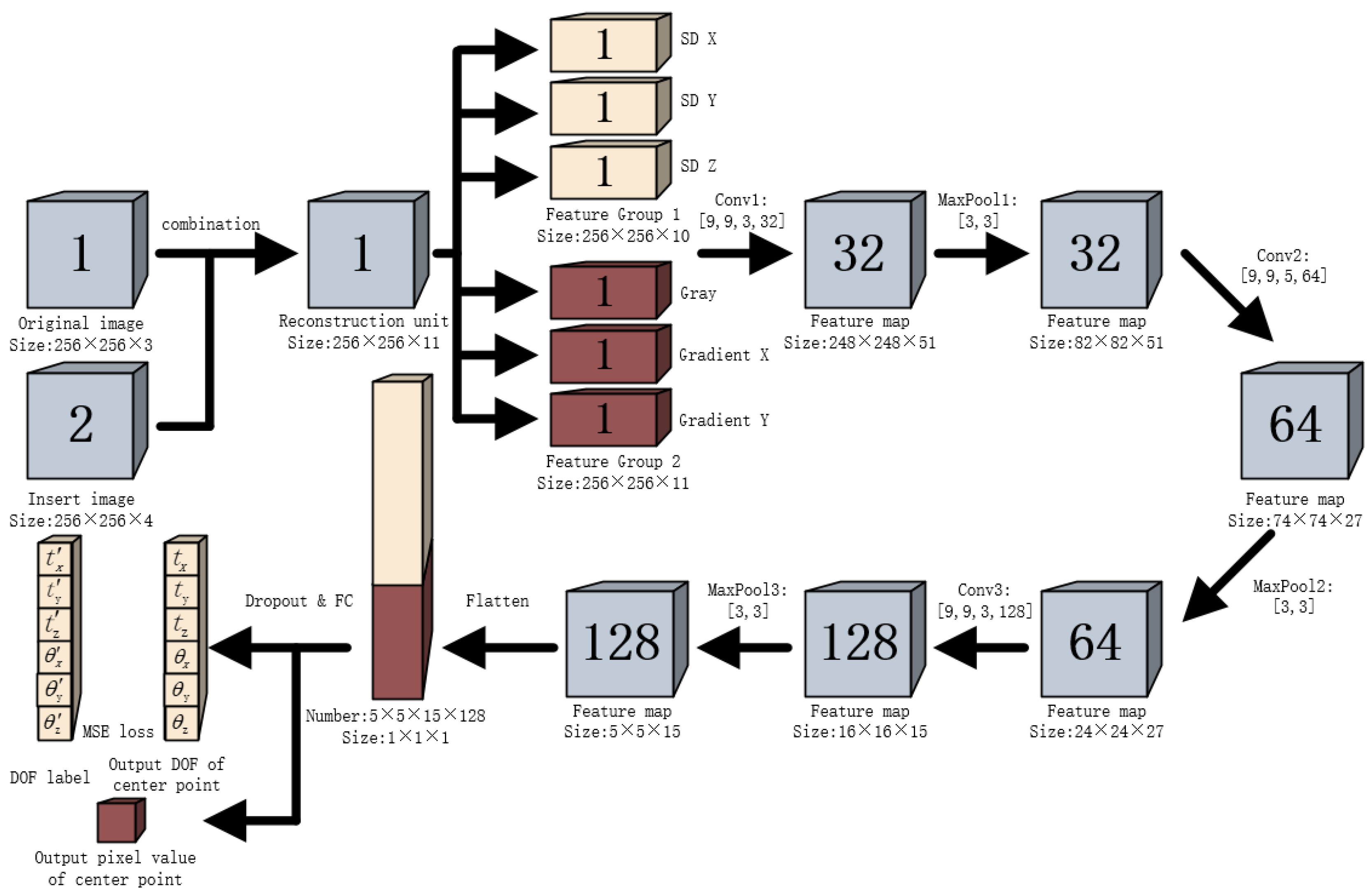
STEP1: Set the ROI of $\mathrm{N}\times \mathrm{M}$ for each B-scan frame in the dataset. Take three $64\times 64$image blocks that are not in the same line from the ROI. Input the B-scan image blocks of each frame into the convolution layer of 3DCNN one by one. STEP2: The speckle decorrelation features of B-scans image blocks are extracted via convolution operation of 3DCNN. The estimated distance of the current two frames of B-scans can be obtained by using the lookup table. STEP3: On the basis of the distance estimation, the normal vectors of the plane where the three image blocks are located are further extracted. Calculate the included angle between the normal vector and the three coordinate axes and the coordinate value of the ROI center point. STEP4: 3DCNN outputs pose information. When training the model, the pose information can be input into LSTM for prediction, which can make MSE reach the minimum value in a short time. After the model training is completed, 3DCNN can run the test set independently without LSTM, show as Figure 6 and Figure 7.

2.3. 3DCNN-LSTM

CNN can automatically extract local features from original data by alternately using convolution and pooling. 3DCNN is an extension of 2DCNN. Not only can it simultaneously capture spatial and temporal features, but it can also generate multiple information channels from adjacent frames. The basic principle of 3DCNN is to execute 2DCNN on each independent information channel. Then, all channel information is synthesized by local connection and shared weight.

A 3DCNN of three-layer convolution constructed in this paper is shown in Figure 6. Among them, the original image is the B-scans directly collected, and the inserted image is the B-scans repeatedly collected according to the interpolation points of the Bezier curve. These two parts constitute the reconstruction unit as the input of the network.

Use ROI to uniformly set the size of each B-scan to $256\times 256$. The size of a single 3D reconstruction unit is $256\times 256\times 11$. The reconstruction unit consists of three B-scans directly acquired and eight B-scans inserted later. The size of the reconstructed volume can be adjusted according to the actual situation. The spatial dimension is represented by $256\times 256$ and 11 represents the time dimension. In other words, 3DCNN operates on 11 B-scans at the same time.

This paper uses the 3D convolution kernel of the deep learning model to extract the B-scans features, and uses LSTM to predict pose offset parameters. As shown in Figure 6, the number of 3D convolution cores is 32, 64 and 128, including $9\times 9\times 5$ and $9\times 9\times 3$. To increase the number of feature maps, the reconstruction unit is copied and divided into two feature groups before 3D convolution. The two feature groups include six different 3D convolutions, which are used to extract features from the reconstructed volume. Feature group 1 includes speckle decorrelation in X, Y and Z directions. These features require two B-scans each time. Feature group 2 includes gradient and grayscale in X and Y directions, which can be directly extracted from a single B-scan. Therefore, the size of feature group 1 is $256\times 256\times 10$, while the size of feature group 2 is $256\times 256\times 11$.

The process of feature extraction is carried out to establish six groups of convolutional filters in 3DCNN to perform local cross-correlation between frames. This process is similar to 2DCNN, and different filters need to be assigned different weights in order to distinguish these. Then, dimension reduction is carried out through a pooling layer to further collect relevant feature information. Finally, reliable features and regions in the image are selected using the relu activation layer.

A pooling layer reduces the computation of convolution. After sampling reduction, the number of feature maps remains unchanged. However, maximum pooling reduces the dimensions of the feature graph. After three episodes of 3D convolution and pooling, a feature map with 128 frames of size of $5\times 5\times 15$is finally obtained. The 1D feature vector data with a length of $5\times 5\times 15\times 128$is obtained from the flat layer and the full connected layer.

In this paper, adaptive motion estimation (Adam) is used to train the model. The convolution weights are initialized randomly and fed back through MSE. The output result includes two parts, the predicted position of ROI middle pixel, and six offset parameters. The pose output of 3DCNN is compared with the real pose, and the MSE loss function is used to represent the difference between the calculation result and the real value.

In order to extract the information in B-scans more accurately, SPRAO combines 3DCNN and LSTM. LSTM is an improved RNN, which can solve the problem of time series prediction. The SPRAO model is shown in Figure 7.

The function of 3DCNN is feature extraction. From the B-scans sequence with a frame rate of 60 FPS, use the sliding window to input 11 frames at a time. According to the inter frame features, 77 features of 11 B-scans are extracted simultaneously, including ROI spatial position sequence and offset parameters. Using freehand collection mode will produce some unavoidable abnormal data. These abnormal data will affect the accuracy of the prediction model; therefore, it is necessary to use exclusion and correction methods to identify bad data and make compensation according to the situation.

The role of LSTM is to make predictions during model training. The sequence constructed from 3DCNN output feature vectors is used as the input data of LSTM. These feature vectors are independent of each other, and temporal features are extracted through LSTM. This paper refers to the expression method of word vector in natural language processing, and connects the characteristics of specific time to form new time series data. The model includes multiple layers of LSTM, and the number of neurons in each layer is 77. Sequence prediction is completed by fully connecting and outputting the data in the specified format. During the experiment, the number of LSTM layers can be adjusted according to the situation to improve the prediction ability of the model.

3. Experimental Setup

3.1. SPRAO System

The hardware of SPRAO experimental system in this paper is shown in Figure 8. The hardware includes a customized handle for fixing a wireless ultrasonic probe and acousto-optic positioning equipment, a positioning base station, positioning information-receiving host, and a processor platform. A customized handle, positioning base station and positioning information-receiving host constitute the positioning system, which can output the pose information of the wireless ultrasonic probe in 3D space. After the positioning system and the wireless probe are fixed, the probe outputs B-scan image sequences containing pose information, which are the input data of SPRAO. The processor platform runs the 3D reconstruction algorithm and compensates the cumulative error of the positioning system.

The specific functions of each hardware are as follows:

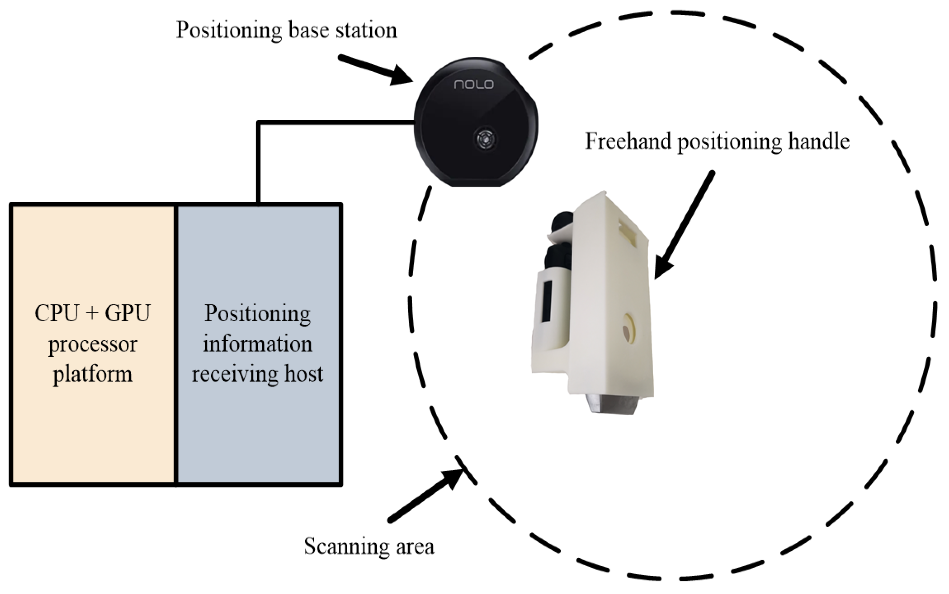
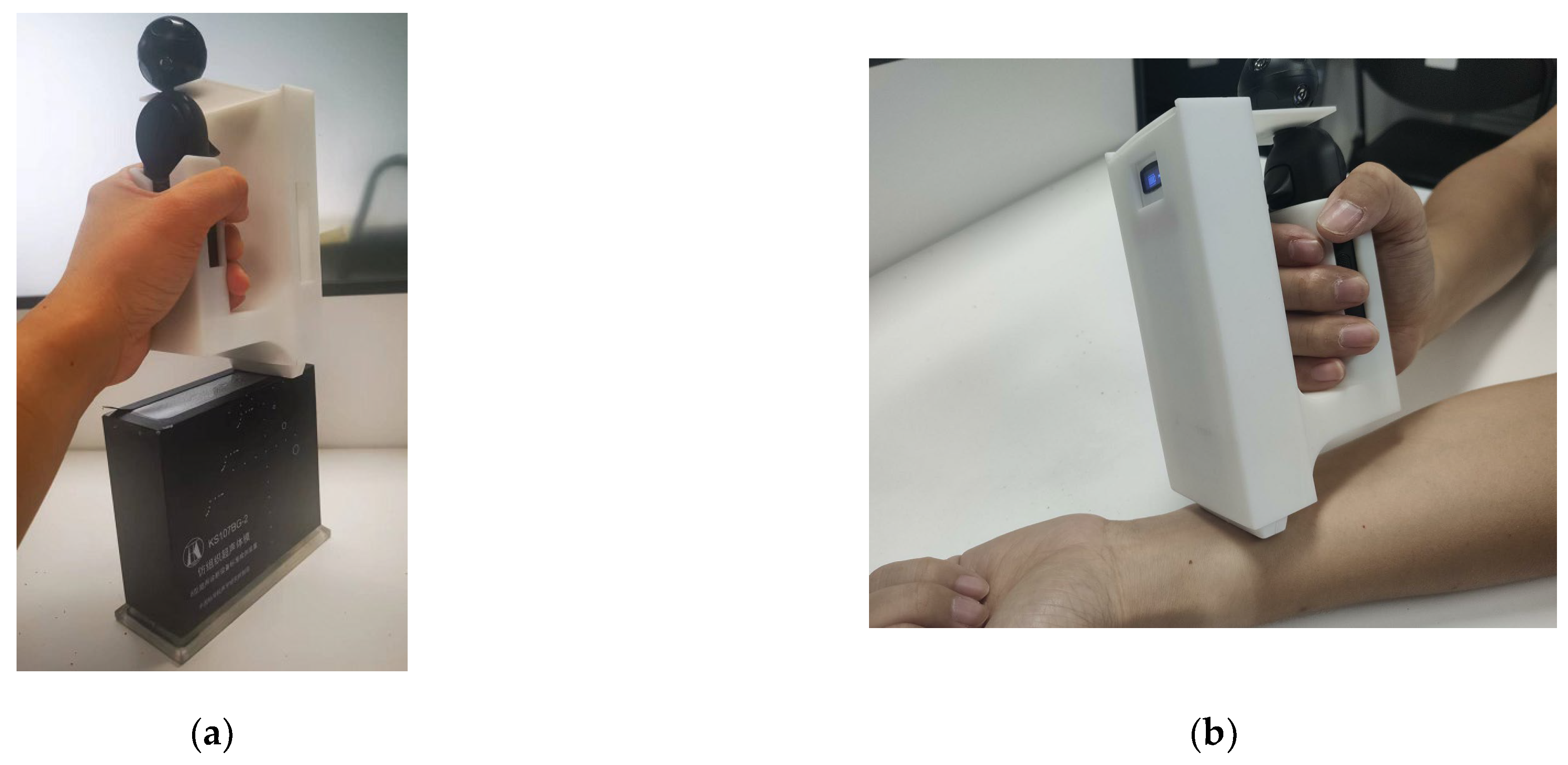
• Customized handle. It is composed of a fixed base, a wireless ultrasonic probe and acousto-optic positioning device, as shown in Figure 9. The wireless probe uses a 128 element linear array probe from Sonostar. The acousto-optic positioning device sends the spatial position coordinates and angle information to the positioning base station, and outputs 60 groups per second. The wireless ultrasonic probe uses a linear array transducer with 128 elements, and uses a 12 FPS frame rate to collect B-scan sequences. The frequency range of the probe is 7–10 MHz, and the depth range is 2–10 cm.
• Positioning base station. The scanning area of the base station needs to be determined. The positioning information of the acousto-optic signal positioning device is transmitted to the positioning information-receiving host through a wire.
• Positioning information-receiving host. Receives the information of the positioning base station. Runs the positioning host visualization software. The software can track the spatial position and angle of the positioning handle in the scanning area.
• Processor platform. Runs the deep learning framework 3DCNN-LSTM. Ubuntu OS runs on Intel (R) Xeon (R) CPU e5-2660. The number of CPUs is 56. The GPU processor model is GeForce RTX 2080, and the number of GPUs is 4. The platform memory capacity is 64 GB, and the solid state disk capacity is 256 GB.

The procedure for using the SPRAO system is as follows.

• Determine the target scanning area of the probe, including the target and path.
• The positioning base station and the positioning information-receiving host are placed in the specified area.
• Connect the positioning information-receiving host and processor platform.

During the model training, the handle is moved repeatedly according to the target path. The 3DCNN-LSTM hybrid network model is imported to predict the spatial position and offset parameters of ROI.

The software components of the SPRAO system have two main programs. Program 1 runs on the positioning host to process the spatial position and angle information. Program 2 runs on the processor platform, training and running the deep learning model 3DCNN-LSTM. Program 1 is developed using unity under a windows system. 3DCNN-LSTM is built and debugged in Python under the ubuntu system. 3DCNN-LSTM uses TensorFlow framework based on the keras deep learning tool.

3.2. Data Acquisition

The data acquisition handle with positioning device is shown in Figure 9. The spatial position parameters of the probe can be returned. Since the positioning device and the actual B-scan plane are not in the same spatial position, it is necessary to perform coordinate transformation on the collected positioning data. The spatial relationship between the actual position of a B-scan and the positioning device is shown in Figure 10. We obtain a set of acousto-optic positioning information $P\left(t_x,t_y,t_z,{\theta }_x,{\theta }_y,{\theta }_z\right)$. Among the data, angle information ${\theta }_x,{\theta }_y,{\theta }_z$, the B-scan angle information, and the coordinate information $t_x,t_y,t_z$ need to be modified according to Figure 10. The corrected B-scan true coordinate information is $P_o\left(t_x,t_y-H,t_z-L,{\theta }_x,{\theta }_y,{\theta }_z\right)$.

The data collection method is shown in Figure 11. First, we define the relevant parameters in the acquisition process. The lateral moving speed of B-scan is $V_s$, and the vertical moving speed is $V_r$. During data collection, $V_s$ and $V_r$ are both 1 cm per second. The probe scans in a straight line. The probe moves at a constant speed close to the target surface. It is necessary to make sure the probe is close to the target surface before moving to a predetermined distance. In this process, the surface and medium changes between the target and the probe will affect the collected data. The movement of the hand-held probe produces uneven pressure on the target surface. When the pressure is high, the noise of the B-scan increases. Therefore, in the acquisition process, the moving direction of the B-scan should be parallel to the target surface as much as possible, and the pressure direction should be vertical to the target surface as much as possible.

3.3. Datasets

Because freehand 3D ultrasound reconstruction is still in the research stage both on national and international levels and has not been put into clinical application, it is impossible to obtain a large number of B-scans data of human tissues with lesion information. The SPRAO algorithm requires more B-scans data with lesions. The loss of ultrasonic propagation in solids is very small. When transmitted to the junction of the metal and the defect, it will be fully or partially reflected. The reflected ultrasonic wave is received by the probe and displays the depth, position and shape of the metal target. Therefore, this paper selects metal targets with different heights, diameters and shapes to construct multiple datasets as simulations. At the same time, human tissue data were collected for verification. As show in Figure 11, the datasets from DB1 to DB4 place different types of metal targets in the ultrasonic phantom to simulate the disease area. Datasets DB5 and DB6 are non-lesion human tissues, mainly used to verify the effect of 3D reconstruction.

According to the above data collection methods, six different targets were selected, and B-scans were collected using an ultrasonic probe to construct six datasets DB1 to DB6, as shown in Figure 12 and

Table 1. Training and test dataset.

Dataset Name	Target	Collection Times	Number of Direct Frames	Number of Interpolation Frames	Moving Track	Average Distance (mm)
DB1	1 mm metal sheet	38	1000	4000	Line	15
DB2	2 mm metal sheet	38	1000	4000	Line	16
DB3	Symmetrical metal block	44	2000	8000	Line	26
DB4	Asymmetric metal block	58	2000	8000	Line	21
DB5	Right of human arm	20	1500	6000	Line	100
DB6	Left of human arm	20	1500	6000	Line	100

. Targets were placed in the ultrasound phantom of Figure 11a for scanning. Among them, the target of DB1 is a metal sheet with a thickness of 1 mm, DB2 is a metal sheet with a thickness of 2 mm, DB3 is a symmetrical metal block with a length of 26 mm, DB4 is an asymmetric metal block with a length of 21 mm, and DB5 and DB6 are human arms which are shown in Figure 11b. The photos of the collection targets of the datasets DB1 to DB4 are shown in Figure 12a–d. Each of the six datasets was made into a training set and a test set at a ratio of 7:3.

In Table 1, direct frames are the 12 FPS B-scans of the wireless probe output. The total number of direct frames and interpolation frames, which is five times the original frame rate, is 60 FPS B-scans, obtained using SPRAO.

In addition, in the process of collecting datasets using a handheld probe, the human arm cannot maintain the same speed movement as the robotic arm. Therefore, the average speed can only be maintained by controlling the total moving distance and total time. Keep $V_r=$ 1 cm/s in Figure 10. The scanning direction of the probe and the normal vector direction of the B-scan plane should be the same. In other words, the ${\theta }_r$ in Figure 10 must be maintained at $90°$ during the acquisition process.

4. Experimental Results

4.1. Bezier Interpolation

Take several fixed points in the Z direction; when the probe passes a certain point, we record the corresponding B-scan and calculate the normal vector of the current B-scan plane. Set the fixed points and B-scans, take four fixed points each time, and calculate a Bezier curve with Equation (1) to complete the interpolation. For example, the result of Bezier interpolation on dataset DB1 is shown in Figure 13. Red dots are the fixed points, and the black line is the Bezier curve calculated according to every four red fixed points. The black curve in Figure 13 is composed of several independent Bezier curves. In practice, it is necessary to interpolate by combining the position of every two red fixed points and the trend of the Bezier curve. The interpolation result is represented by the blue points in Figure 13. As you can see, four blue dots are inserted between every two red fixed points. The red dots and blue dots constitute the space acquisition coordinates of B-scans. There are still some errors between the coordinates of these inserted B-scans and the real values. The error will be adjusted later by the speckle decorrelation of SPRAO.

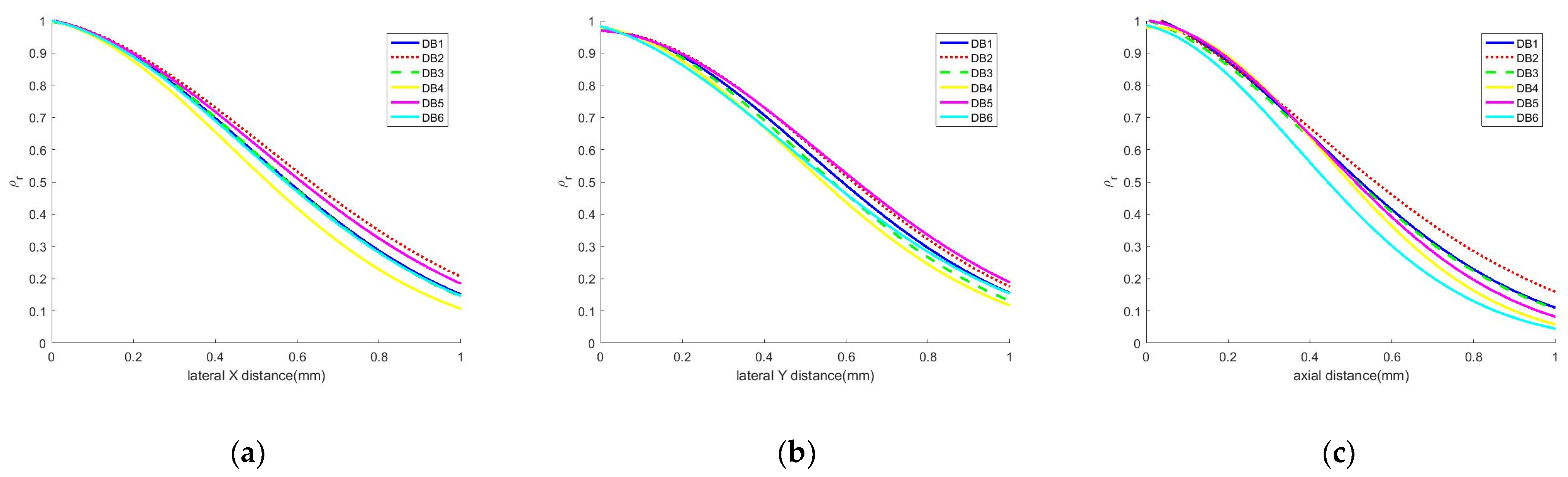
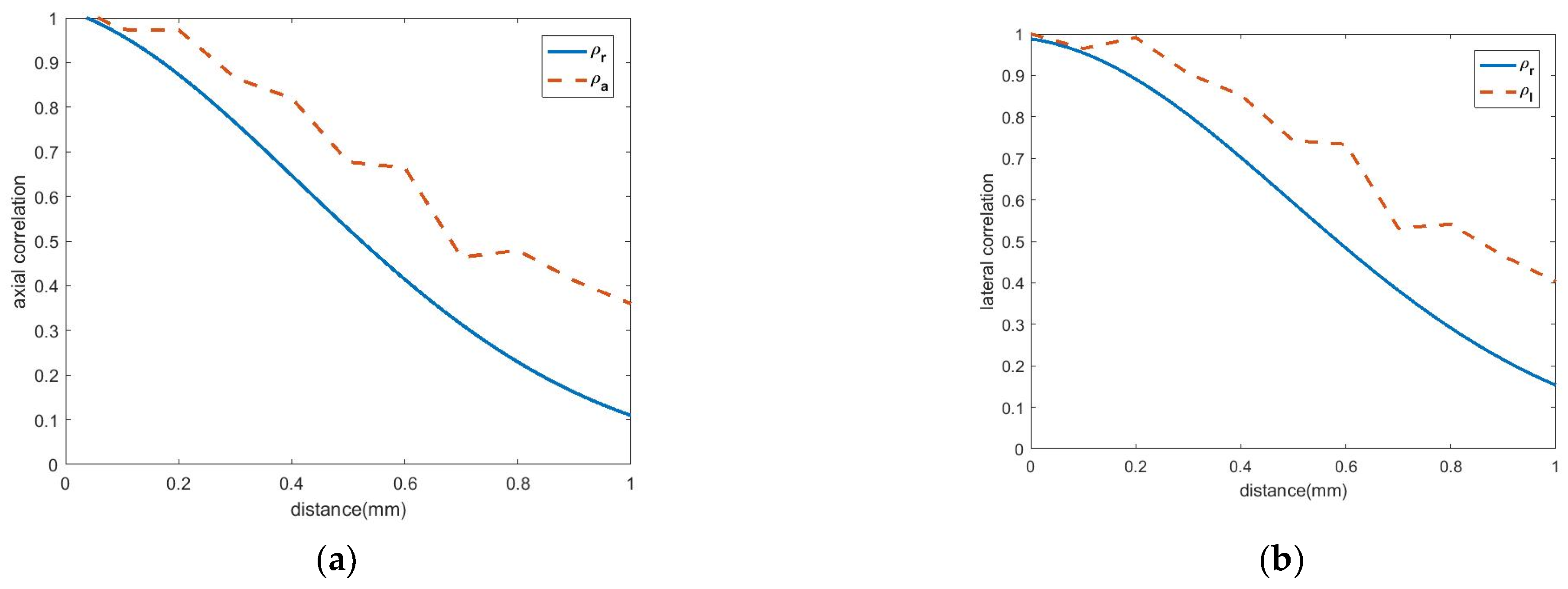
4.2. Speckle Decorrelation Calibration Curve

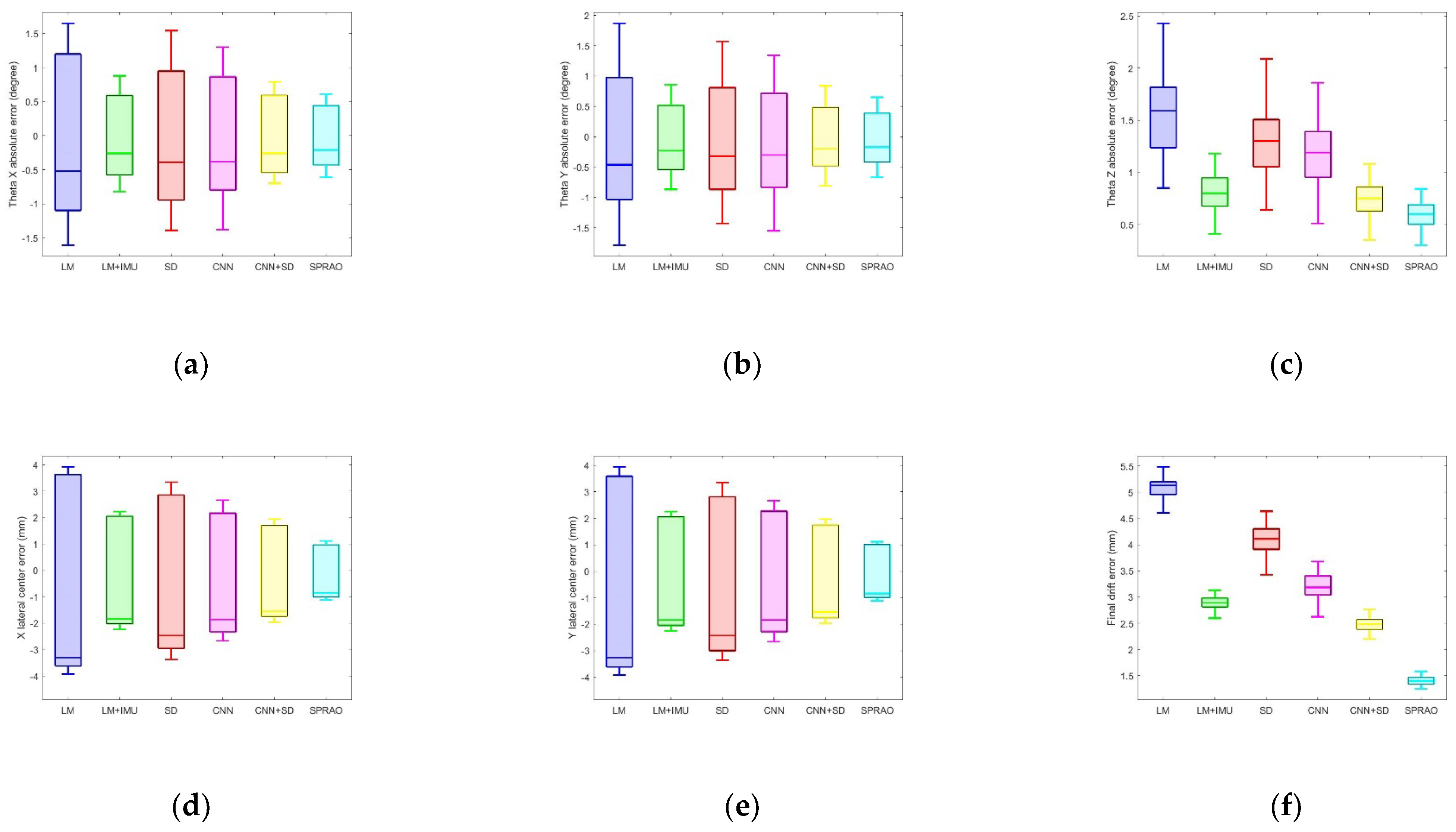
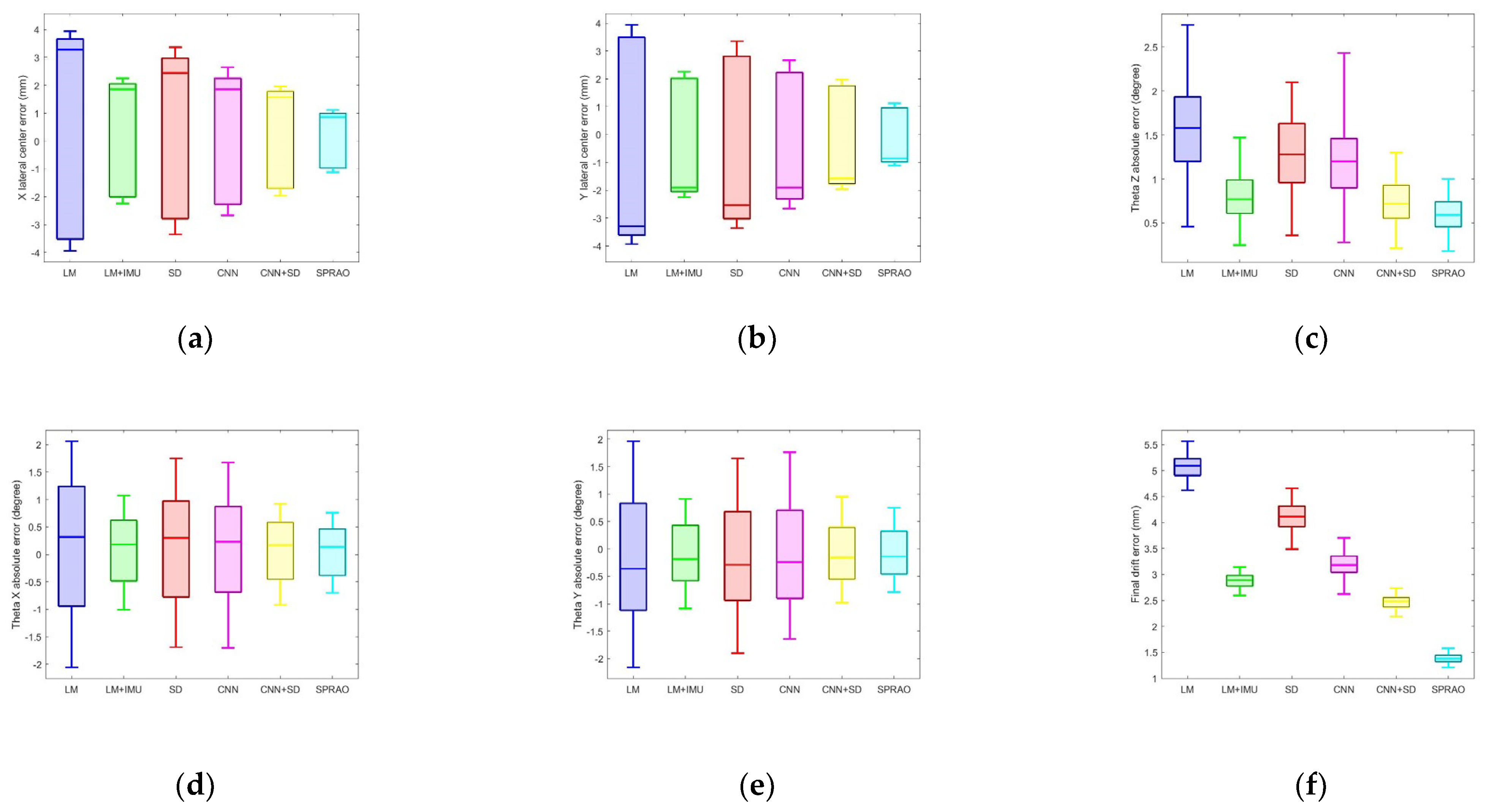
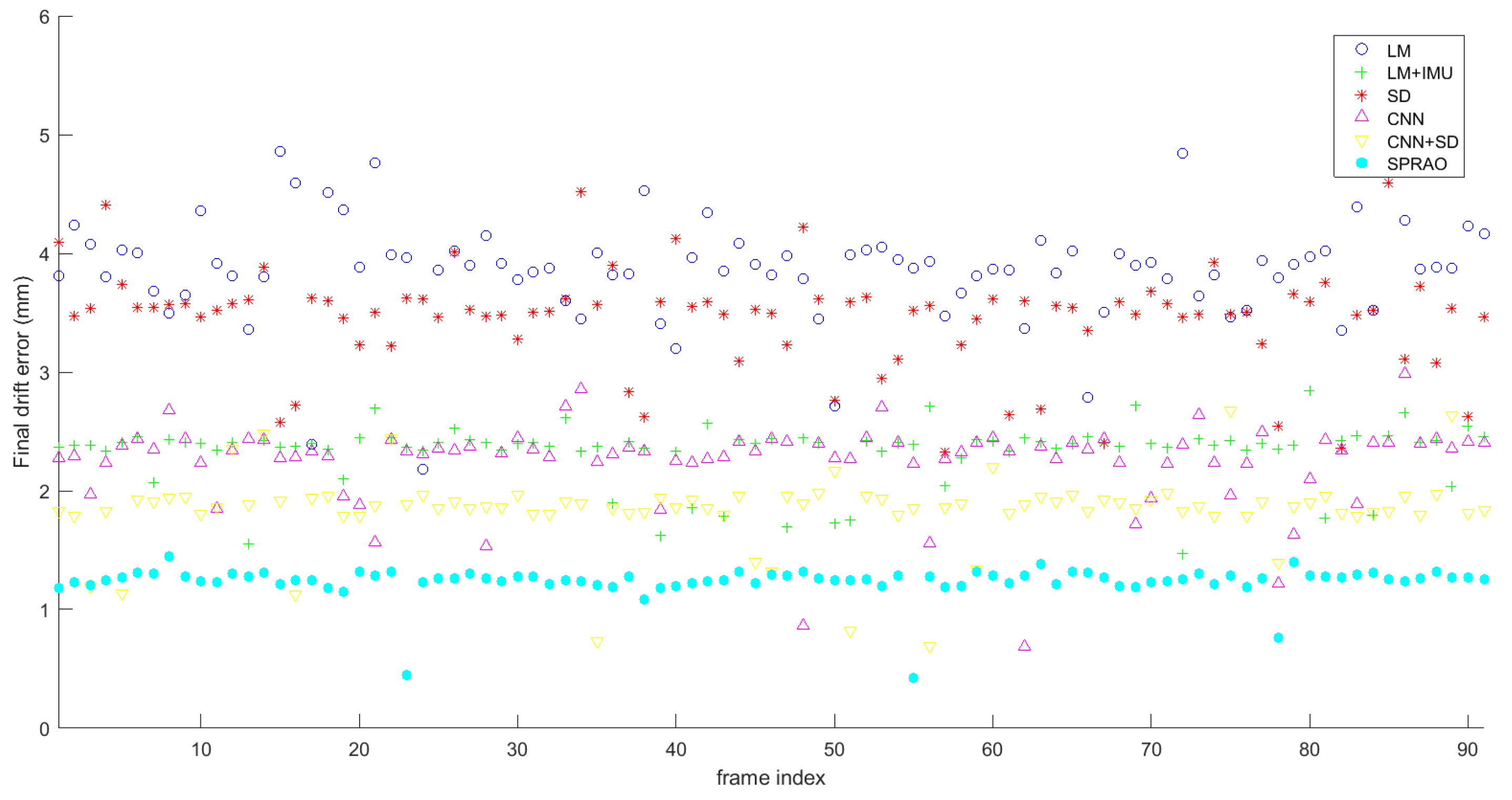
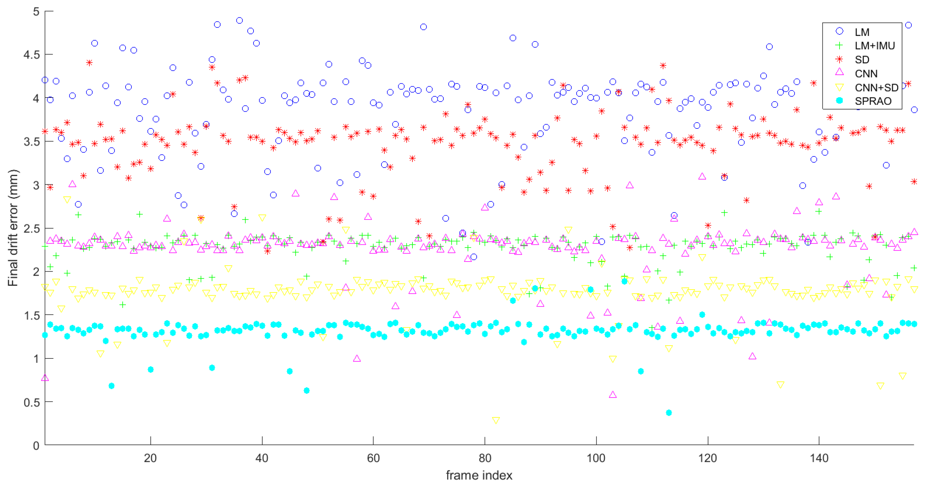
The speckle calibration curve is the first step in training the 3DCNN model. The ultrasonic probe needs to be fixed on a three-axis motion platform for acquisition. The probe moves in the range of 0–1 mm along the axial and lateral direction. According to the coordinate points of Bezier interpolation, record the spatial position of the B-scans, and use Equation (4) to calculate the correlation coefficients of three 64 $\times$ 64 image blocks in the ROI of adjacent two frames of B-scans, as shown in Figure 14.

The displacement correlation curves obtained by calibrating six datasets are shown in Figure 15. It can be seen that the change trend of the calibration curve of the same probe in different datasets is similar. With the displacement correlation curve, as long as the correlation between three image blocks is not in the same, the straight line position on two B-scans is calculated, and the corresponding distance value can be obtained. Then, calculate the displacement of the B-Scan plane normal vector. With the calibration curve, in the subsequent steps of SPRAO, Equations (5) and (6) can be used to calculate the displacement value of the true speckle autocorrelation between two B-scans frames according to the value of ${\rho }_r$.

4.3. SPRAO

In Figure 7, 70% of the 60 PFS dataset is used as the training set. A fixed number of B-scans from the training set are input into the 3DCNN-LSTM network for training each time. After the training, it is only necessary to convert the spatial position of the continuous B-scans to the 3D absolute coordinate system according to the method in Figure 2 and through LSTM to repeatedly estimate and predict the offset parameters relative to the previous frame image; thus, the spatial position and angle of the B-scans sequence in the 3D volume can be obtained.

The distance estimation of SPRAO speckle decorrelation is completed in 3DCNN. Using the estimated distance of the three non-collinear image blocks on the current B-scan from the previous frame, the spatial position of the current B-scan can be determined. In this process, Equation (4) is used to calculate the displacement correlation coefficient ${\rho }_a$ curve and ${\rho }_l$ curve of coherent interference, where a is the axial correlation coefficient and l is the lateral correlation coefficient. Taking dataset DB1 as an example, the curve of the axial and lateral variation with distance is shown in Figure 16, where the lateral correlation coefficient ${\rho }_l$ is the combination of the X and Y directions. According to the curve and table lookup method in Figure 16, the curves of $k_a$ and $k_l$ can be calculated using Equations (5) and (6). The curves of $k_a$ and $k_l$ for dataset DB1 are shown in Figure 17.

It can be seen from the experimental results that axial $k_a$and lateral $k_l$are equally important in the actual acquisition process. Therefore, take the average of $k_a$ and $k_l$ as the final estimate $k_e$. The $k_e$ curves calculated from each of the six datasets are shown in Figure 18.

Finally, ${\rho }_e$ is calculated by looking up the table and Equations (5) and (6). ${\rho }_e$ is the corrected displacement evaluation curve, which is close to the ground truth. The ${\rho }_e$ curves of the six datasets are shown in Figure 19 and Figure 20. With these curves, the current actual displacement can be obtained from the corresponding ${\rho }_e$ curve by calculating the speckle decorrelation coefficient of two frames of B-scans.

Figure 6 and Figure 7 are the process of training the model using the training set. LSTM is used to predict the output pose information of 3DCNN so that MSE can reach the minimum value in a short time. LSTM can speed up the training process of the model. When the model training is completed, 3DCNN can be separated from LSTM and used alone to output the pose information within the expected error.

Firstly, when training the model, the training set of the same dataset is cloned from one to six copies. Six different convolution kernels are used in the convolution layer of 3DCNN, as shown in Figure 6 and Figure 7. Then, three convolution operations are performed on the B-scans sequence in the training set to complete the inter-frame speckle decorrelation, gradient and grayscale operations. Finally, through the pooling layer and activation layer of 3DCNN, the elimination of abnormal pose data and the lookup table process of displacement correlation coefficient are completed, as shown in Figure 19 and Figure 20.

In this process, 3DCNN extracts the speckle decorrelation features of 60 FPS B-scans, and calculates the MSE of each frame B-scan and the true value. The 3DCNN outputs a 1D pose information array of $5\times 5\times 15\times 128$. When there is no LSTM in the training process, it takes a considerable amount of time to adjust the parameters of 3DCNN to minimize MSE according to the MSE of the output pose information array. LSTM predicts the pose information of the next set of B-scans sequences based on the current B-scans sequence pose information. As shown in Figure 7, the prediction results of LSTM and the next set of 60 FPS B-scans are used as input of 3DCNN. Combining the prediction information of LSTM, 3DCNN continues to complete the inter-frame speckle decorrelation, gradient and grayscale operations, and calculates the MSE of each frame B-scan and the true value. In the same training times, different MSE error can be obtained by changing the number of LSTM layers in Figure 7. The experimental results are shown in

Table 2. Number of layers of LSTM and prediction results.

Number of LSTM Layers	Training Times	MSE Error
2	500	3.2%
4	500	3.1%
5	500	2.5%
6	500	2.1%
7	500	1.8%
8	500	2.0%

. It can be seen that increasing the number of LSTM layers can improve the prediction ability; however, when the number of LSTM layers increases to eight, the training error increases. Therefore, SPRAO chooses seven layers LSTM in the training process. The MSE in Table 2 is obtained through the average of all B-scans pose deviations, including ROI center point gray level offset and six pose parameter offset, as shown in Figure 6.

After completing the model training, the test set can be input into 3DCNN without LSTM. 3DCNN outputs the characteristics of speckle decorrelation and gradient in both axial and lateral directions of B-scan. At the same time, the gray level of the center point is output. Linear motion (LM), linear motion with IMU (LM + IMU), speckle decorrelation (SD), CNN, CNN combined with speckle decorrelation (CNN + SD) and SPRAO are used for DB1, DB3 and DB5 datasets in Table 2. The experimental results are shown in Figure 21, Figure 22 and Figure 23 using box plots. In each Figure, different boxes use different colors, represent LM, LM + IMU, SD, CNN, CNN + SD and SPRAO. The absolute error of all B-scans in a single dataset under different methods is represented by six sub figures. Subfigure (a), (b) and (c) are the absolute angular errors of the B-scan plane normal vector and the coordinate axes X, Y, and Z, as shown in Figure 3 and Figure 5. Subfigure (d) and (e) are the absolute error of the offset distance of the B-scan center point in the two directions of Lateral X and Lateral Y, as shown in Figure 5 and Figure 20. Subfigure (f) is the final drift error of the dataset, that is, MSE which is output by 3DCNN-LSTM.

5. Discussion

In this part, SPRAO is compared with linear motion (LM), LM + IMU, speckle decorrelation (SD) and CNN + SD. According to the experimental results of different methods, the differences between the proposed method SPARO and other related works are discussed. It can be seen that the spatial pose deviation of B-scans output by SPRAO is the best of these methods.

Firstly, box plots are used to compare the intermediate variables of different methods in the process of 3D reconstruction. It can be seen from the diagram that the LM method has a large range of intermediate data errors due to lack of feedback. Since some intermediate data errors cancel each other out in the calculation process, the MSE error of LM does not look so large; however, it is still the largest compared to other methods. The LM + IMU method uses high-precision IMU to provide feedback for LM, which can effectively reduce errors.

Because the SD method relies only on the speckle decorrelation of B-scans, the error performance of the intermediate data of SD is similar to that of LM, and its MSE error is larger than that of LM. If we only analyze (a), (b) and (c) in Figure 21, Figure 22 and Figure 23, we can see that the absolute angular errors of SPARO, LM + IMU and CNN + SD in the normal vector of B-scan plane are almost the same. From (e), (f) and (g) in Figure 21, Figure 22 and Figure 23, we can see that when calculating lateral distance and drift, the output error of SPARO is significantly reduced compared with other methods. In addition, the dataset of DB5 in Table 2 is large; therefore, the SPARO performance is improved when the size of the dataset increases. This is also why box plots are used.

Secondly, the absolute angular errors, absolute offset distance errors and final drift errors of DB1, DB3, DB5 and DB6 under different methods are shown in

Table 3. Comparison of average error and final drift of different methods.

DB1 Methods	Average Error (mm/°)					Final Drift (mm)
	X	Y	${\theta }_x$	${\theta }_y$	${\theta }_z$	Min.	Med.	Max.
Linear motion (LM)	3.94	3.87	1.69	1.81	2.38	2.23	3.92	5.19
LM + IMU	2.25	2.23	0.87	0.91	1.19	1.59	2.4	3.08
Speckle decorrelation (SD)	3.35	3.33	1.53	1.37	1.87	2.4	3.54	4.51
CNN	2.52	2.52	1.36	1.45	1.85	0.89	2.34	3.45
CNN + SD	2.23	2.23	0.79	0.85	1.05	0.29	1.88	2.9
SPRAO	1.55	1.55	0.61	0.67	0.83	0.41	1.25	1.98
DB3 Methods	Average Error (mm/°)					Final Drift (mm)
	X	Y	${\theta }_x$	${\theta }_y$	${\theta }_z$	Min.	Med.	Max.
Linear motion (LM)	3.92	3.87	2.05	2.15	2.86	2.35	4.07	5.4
LM + IMU	2.25	2.25	1.06	1.01	1.44	1.58	2.34	3.13
Speckle decorrelation (SD)	3.37	3.37	1.79	1.91	2.28	2.48	3.56	4.67
CNN	2.54	2.54	1.66	1.8	2.05	0.83	2.33	3.39
CNN + SD	2.2	2.21	0.96	0.98	1.31	0.42	1.8	2.95
SPRAO	1.53	1.55	0.75	0.75	1.03	0.26	1.33	2.14
DB5 Methods	Average Error (mm/°)					Final Drift (mm)
	X	Y	${\theta }_x$	${\theta }_y$	${\theta }_z$	Min.	Med.	Max.
Linear motion (LM)	3.94	3.94	3.18	3	3.93	2.25	3.98	5.52
LM + IMU	2.25	2.25	1.65	1.49	2.1	1.43	2.34	3.16
Speckle decorrelation (SD)	3.37	3.37	2.77	2.57	3.53	2.25	3.54	4.66
CNN	2.54	2.54	2.6	2.45	3.09	0.87	2.32	3.48
CNN + SD	2.25	2.25	1.48	1.35	1.85	0.35	1.84	3.17
SPRAO	1.55	1.55	1.16	1.05	1.44	0.26	1.3	2.15
DB6 Methods	Average Error (mm/°)					Final Drift (mm)
	X	Y	${\theta }_x$	${\theta }_y$	${\theta }_z$	Min.	Med.	Max.
Linear motion (LM)	3.94	3.92	3.18	3.03	4.34	2.28	4.02	5.49
LM + IMU	2.25	2.25	1.57	1.55	2.03	1.46	2.37	3.14
Speckle decorrelation (SD)	3.37	3.37	2.8	2.7	3.48	2.24	3.53	4.68
CNN	2.54	2.54	2.52	2.48	3.15	0.81	2.31	3.51
CNN + SD	2.25	2.25	1.45	1.41	1.89	0.23	1.81	3.14
SPRAO	1.55	1.53	1.1	1.07	1.49	0.2	1.31	2.16

. The absolute angle error, absolute offset distance error and final drift error will have an important impact on the effect of 3D reconstruction. Final drift errors include maximum, intermediate and minimum. The unit of X, Y and final drift is mm, and the unit of ${\theta }_x$, ${\theta }_y$ and ${\theta }_z$ is degree.

Thirdly, the final drift error of each frame of B-scan is graphically plotted using scatter plot. The final drive performance of each dataset under different methods is shown in Figure 24, Figure 25, Figure 26 and Figure 27. X-axis is ground truth and Y-axis is the results of other models. It can be seen that although the variation range of final drive of SPRAO under different datasets is not the smallest, the average error performance is the best. The error of the final drive is small; therefore, each B-scan can be placed in the correct position in the 3D space, making the reconstruction result more realistic. At the same time, the Pearson correlation coefficient (PCC), R2, MSE, and MAS are added to describe the fitting effect of the prediction results, as shown in

Table 4. Different evaluation methods compare the prediction results and fitting effects.

Results of Dataset DB1	PCC	R2	MSE	MAS
Linear motion (LM)	−0.17	−0.04	14.75	3.79
LM + IMU	0.13	0.83	5.57	2.35
Speckle decorrelation (SD)	−0.13	0.51	11.66	3.39
CNN	0.23	0.84	7.75	2.29
CNN + SD	−0.02	0.69	3.29	1.78
SPRAO	0.25	0.94	1.55	1.24
Results of Dataset DB3	PCC	R2	MSE	MAS
Linear motion (LM)	0.14	0.02	14.72	3.79
LM + IMU	−0.16	0.88	5.22	2.28
Speckle decorrelation (SD)	0.12	0.67	12.28	3.49
CNN	0.19	0.79	7.91	2.26
CNN + SD	0.22	0.76	3.09	1.74
SPRAO	0.45	0.89	1.67	1.28
Results of Dataset DB5	PCC	R2	MSE	MAS
Linear motion (LM)	0.17	0.03	14.08	3.71
LM + IMU	0.29	0.75	4.99	2.21
Speckle decorrelation (SD)	0.14	0.46	11.28	3.33
CNN	0.23	0.77	7.28	2.18
CNN + SD	0.41	0.71	3.19	1.76
SPRAO	0.55	0.91	1.63	1.26
Results of Dataset DB6	PCC	R2	MSE	MAS
Linear motion (LM)	0.17	0.03	2.05	2.15
LM + IMU	0.26	0.76	1.06	1.01
Speckle decorrelation (SD)	0.19	0.56	1.79	1.91
CNN	0.27	0.81	1.36	1.45
CNN + SD	0.29	0.66	0.79	0.85
SPRAO	0.53	0.91	0.61	0.67

.

It can be observed in Table 4 that the prediction results of LM + IMU, CNN, CNN + SD and SPRAO are well-fitted. However, compared with other methods, SPRAO adds LSTM for prediction. Therefore, the MSE and MAS of SPRAO perform better. The closer PCC is to 1, the smaller MSE deviates from ground truth. It can be seen that the PCC results of the six methods are not very good. The table also reflects that the R2 value of the prediction result and the ground truth fitting result is not the same as the PCC. It is mainly due to the error of freehand movement in space and the change of target surface due to extrusion. Because the cause of the error is fully considered and corrected, the PCC and R2 of SPRAO are better than other methods.

Finally, the effect of Bezier interpolation and speckle decorrelation in SPRAO algorithm is demonstrated in the 3D reconstruction results. Figure 28, Figure 29 and Figure 30 are the results of 3D ultrasound reconstruction of DB3. Figure 28 is the result of 12PFS B-scans without Bezier interpolation. Because the frame rate is not high, the reconstruction results lose more details. Figure 29 is the result of 60PFS B-scans using only Bezier interpolation. Figure 29 does not perform speckle decorrelation operation. The frame rate after interpolation is five times that of the original, and more details can be obtained. However, because the interpolation is based on the fitted Bezier curve, there is a certain error between the inserted B-scans and the real position. Figure 30 shows the results of 3D ultrasound reconstruction using SPRAO in DB3.

6. Conclusions

In this paper, a wireless linear array probe is used to build a freehand acousto-optic positioning 3D ultrasonic imaging system, using this system to collect and construct multiple 2D B-scans datasets for experiments. According to the experimental results, a freehand 3D ultrasonic reconstruction method based on depth learning is proposed, which is called sequence prediction reconstruction based on acoustic optical localization (SPRAO). Compared with other freehand 3D reconstruction methods without SPRAO, the proposed method has three advantages:

(1)

The doctor can obtain 60 FPS B-scans of the target through 2–3 continuous acquisitions. Limited by the speed of the wireless transmission chip, the wireless probe can only output 12 FPS. If SPRAO is not used, the doctor needs to stay for a few seconds after each movement of the probe to ensure that the target B-scans are collected. When using SPRAO, three Bezier curves are fitted from the existing 12 frames of B-scans according to the pose. From the experimental results of Bezier interpolation, it can be seen that the output of 60 FPS can be synthesized by inserting four points between two B-scans of each Bezier curve and using the speckle decorrelation between B-scans for pose calibration. This not only effectively reduces the requirement for the output frame rate of the ultrasonic probe, but also increases the moving speed of the wireless probe.

(2)

The cumulative error can be compensated by the speckle decorrelation between two frames of B-scans. Firstly, the positioning information output by the acousto-optic positioning device is not easily affected by obstacles. Secondly, setting ROI to extract the speckle decorrelation features of two B-scans can not only help to construct 60 FPS B-scans output, but also calibrate the cumulative error of acousto-optic auxiliary positioning information.

(3)

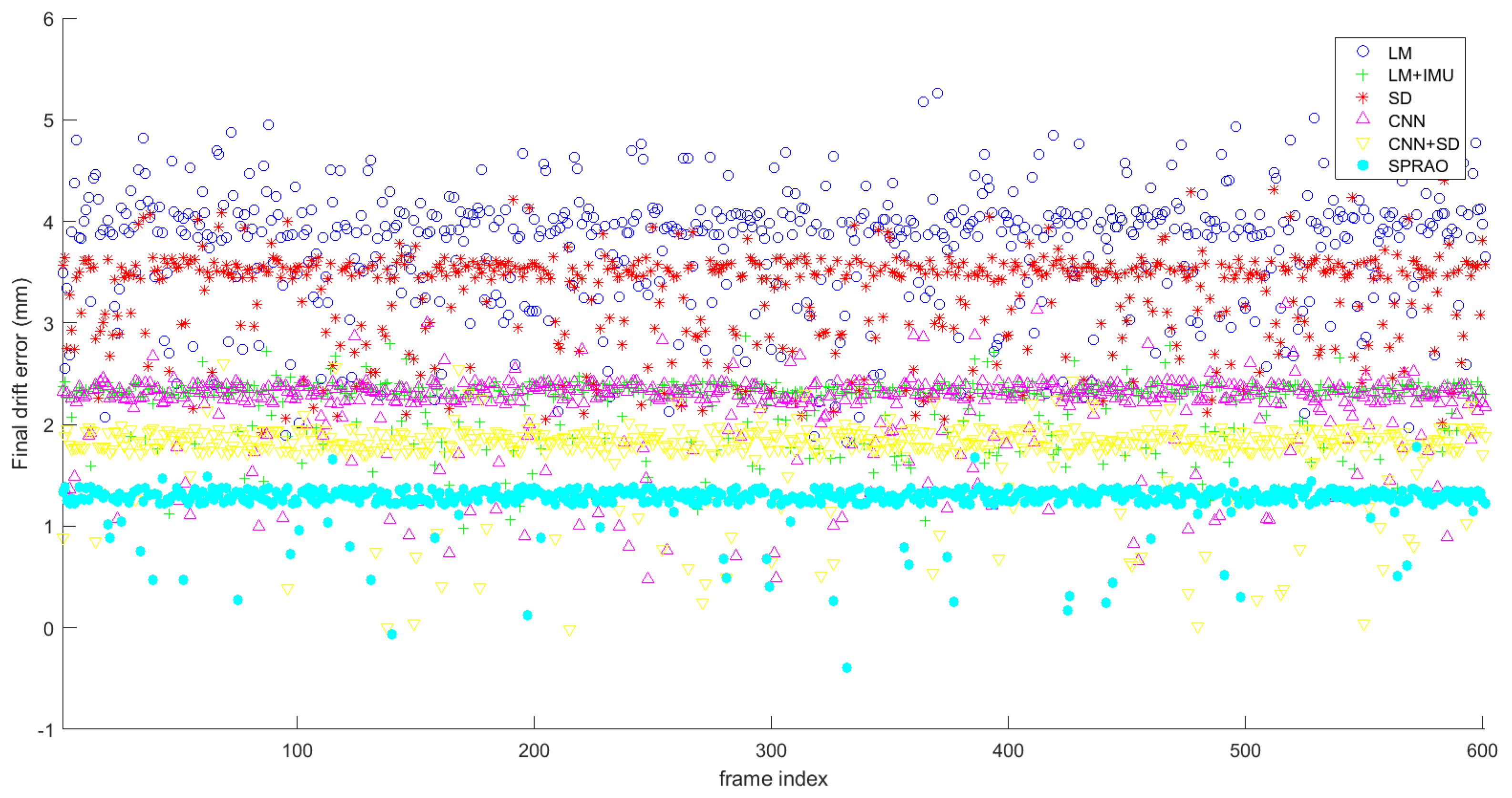
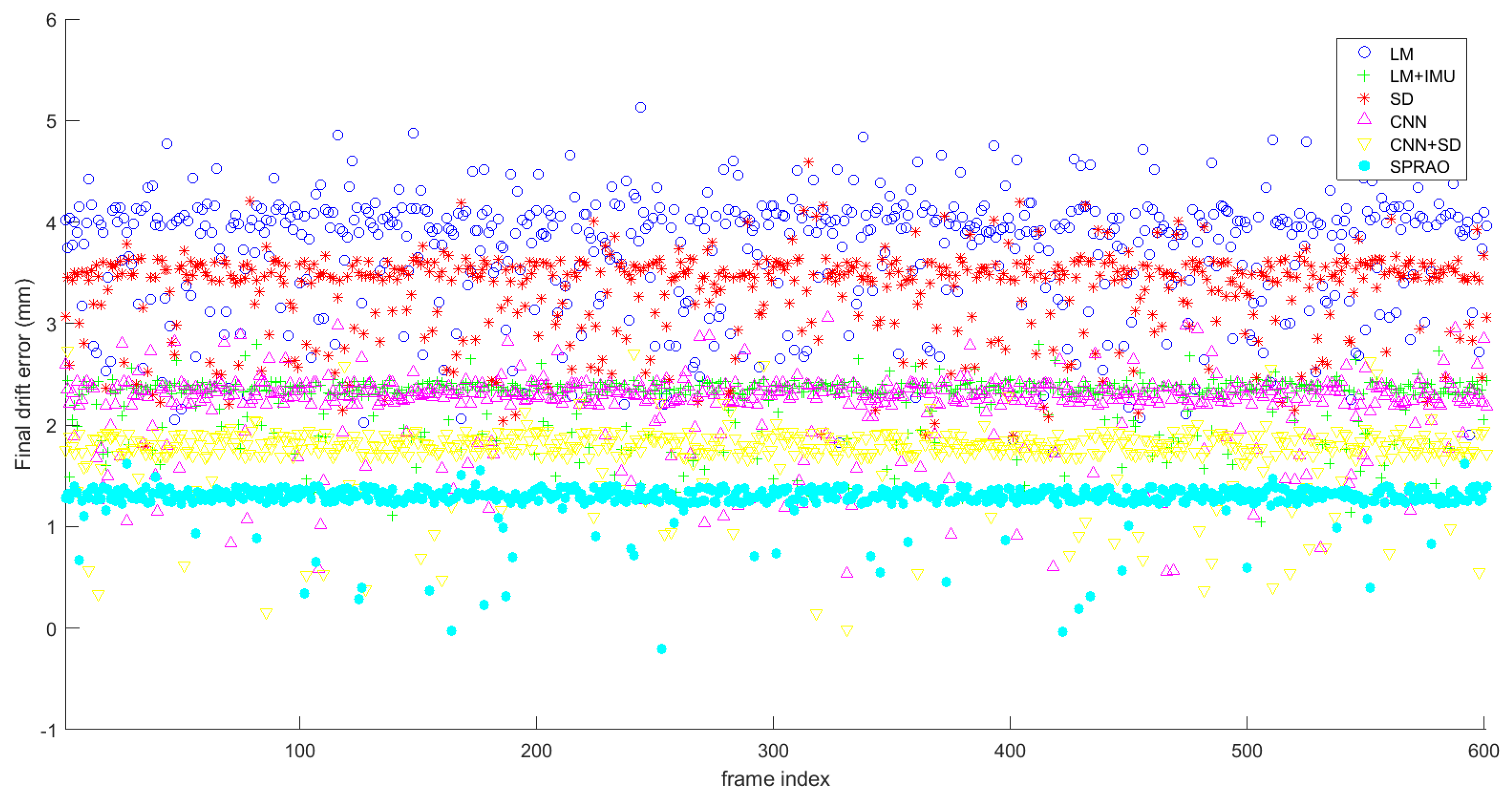
3DCNN-LSTM reduces the time for MSE to reach the target value. It provides the necessary conditions for real-time 3D reconstruction. Without deep learning, in order to obtain more B-scans, the probe must stay for several seconds after each move to complete the acquisition and reconstruction. In this paper, 3DCNN-LSTM model is used to improve the efficiency of B-scans sequence feature extraction. The calculation of pose deviation and speckle decorrelation is integrated into 3DCNN. The LSTM predicts the output pose information of the 3DCNN, which makes the MSE reach the minimum value in a short time. The experimental results not only show that the deep learning model can track the spatial pose change of B-scans better than other methods, but also that the MSE of the test dataset is less than 2.5 mm.

The future work will focus on SPRAO. Optimize the 3DCNN-LSTM model to improve the real-time performance of SPRAO. At the same time, the number of features and calibration curves extracted during the training process will be further reduced, and a lighter model will be constructed for the embedded platform.

References

1. Mohamed, F.; Chan, V.S. A Survey on 3D Ultrasound Reconstruction Techniques. In Artificial Intelligence—Applications in Medicine and Biology; IntechOpen: London, UK, 2019. [Google Scholar]
2. Mozaffari, M.H.; Lee, W.-S. Freehand 3-D Ultrasound Imaging: A Systematic Review. Ultrasound Med. Biol. 2017, 43, 2099–2124. [Google Scholar] [CrossRef] [PubMed] [Green Version]
3. Song, F.; Ma, Y.; You, I.; Zhang, H. Smart Collaborative Evolvement for Virtual Group Creation in Customized Industrial IoT. IEEE Trans. Netw. Sci. Eng. 2022, 1–11. [Google Scholar] [CrossRef]
4. Song, F.; Zhu, M.; Zhou, Y.; You, I.; Zhang, H. Smart Collaborative Tracking for Ubiquitous Power IoT in Edge-Cloud Interplay Domain. IEEE Internet Things J. 2019, 7, 6046–6055. [Google Scholar] [CrossRef]
5. Hsu, P.W. Freehand Three—Dimensional Ultrasound Calibration; University of Cambridge: Cambridge, UK, 2008. [Google Scholar]
6. Huang, Q.; Zeng, Z. A Review on Real-Time 3D Ultrasound Imaging Technology. BioMed Res. Int. 2017, 2017, 6027029. [Google Scholar] [CrossRef] [Green Version]
7. Moon, H.; Ju, G.; Park, S.; Shin, H. 3D freehand ultrasound reconstruction using a piecewise smooth Markov random field. Comput. Vis. Image Underst. 2016, 151, 101–113. [Google Scholar] [CrossRef]
8. Toonkum, P.; Suwanwela, N.C.; Chinrungrueng, C. Reconstruction of 3D ultrasound images based on Cyclic Regularized Savitzky–Golay filters. Ultrasonics 2011, 51, 136–147. [Google Scholar] [CrossRef]
9. Huang, Q.-H.; Yang, Z.; Hu, W.; Jin, L.-W.; Wei, G.; Li, X. Linear Tracking for 3-D Medical Ultrasound Imaging. IEEE Trans. Cybern. 2013, 43, 1747–1754. [Google Scholar] [CrossRef] [PubMed]
10. Huang, Q.; Wu, B.; Lan, J.; Li, X. Fully Automatic Three-Dimensional Ultrasound Imaging Based on Conventional B-Scan. IEEE Trans. Biomed. Circuits Syst. 2018, 12, 426–436. [Google Scholar] [CrossRef] [PubMed]
11. Huang, Q.; Lan, J.; Li, X. Robotic Arm Based Automatic Ultrasound Scanning for Three-Dimensional Imaging. IEEE Trans. Ind. Inform. 2019, 15, 1173–1182. [Google Scholar] [CrossRef]
12. Chung, S.-W.; Shih, C.-C.; Huang, C.-C. Freehand three-dimensional ultrasound imaging of carotid artery using motion tracking technology. Ultrasonics 2017, 74, 11–20. [Google Scholar] [CrossRef]
13. Cenni, F.; Monari, D.; Desloovere, K.; Aertbeliën, E.; Schless, S.-H.; Bruyninckx, H. The reliability and validity of a clinical 3D freehand ultrasound system. Comput. Methods Programs Biomed. 2016, 136, 179–187. [Google Scholar] [CrossRef] [PubMed]
14. Herickhoff, C.; Lin, J.; Dahl, J. Low-cost Sensor-enabled Freehand 3D Ultrasound. In Proceedings of the 2019 IEEE International Ultrasonics Symposium (IUS), Glasgow, UK, 6–9 October 2019. [Google Scholar]
15. Chen, X.; Chen, H.; Peng, Y.; Tao, D. Probe Sector Matching for Freehand 3D Ultrasound Reconstruction. Sensors 2020, 20, 3146. [Google Scholar] [CrossRef]
16. Daoud, M.I.; Alshalalfah, A.L.; Awwad, F.; Al-Najar, M. Freehand 3D Ultrasound Imaging System Using Electromagnetic Tracking. In Proceedings of the 2015 International Conference on Open Source Software Computing, Amman, Jordan, 10–13 September 2015. [Google Scholar]
17. Wen, T.; Yang, F.; Gu, J.; Wang, L. A novel Bayesian-based nonlocal reconstruction method for freehand 3D ultrasound imaging. Neurocomputing 2015, 168, 104–118. [Google Scholar] [CrossRef]
18. Mohamed, F.; Mong, W.S.; Yusoff, Y.A. Quaternion Based Freehand 3D Baby Phantom Reconstruction Using 2D Ultrasound Probe and Game Controller Motion and Positioning Sensors. In Proceedings of the International Conference for Innovation in Biomedical Engineering & Life Sciences, ICIBEL 2015, Putrajaya, Malaysia, 6–8 December 2015; Springer: Singapore, 2015. [Google Scholar]
19. Gao, H.; Huang, Q.; Xu, X.; Li, X. Wireless and sensorless 3D ultrasound imaging. Neurocomputing 2016, 195, 159–171. [Google Scholar] [CrossRef]
20. Afsham, N.; Rasoulian, A.; Najafi, M.; Abolmaesumi, P.; Rohling, R. Nonlocal means filter-based speckle tracking. IEEE Trans. Ultrason. Ferroelectr. Freq. Control 2015, 62, 1501–1515. [Google Scholar] [CrossRef] [PubMed]
21. Coupe, P.; Hellier, P.; Kervrann, C.; Barillot, C. Nonlocal means-based speckle filtering for ultrasound images. IEEE Trans. Image Process. 2009, 18, 2221–2229. [Google Scholar] [CrossRef] [PubMed] [Green Version]
22. Song, F.; Ai, Z.; Zhang, H.; You, I.; Li, S. Smart Collaborative Balancing for Dependable Network Components in Cyber-Physical Systems. IEEE Trans. Ind. Inf. 2021, 17, 6916–6924. [Google Scholar] [CrossRef]
23. Song, F.; Zhou, Y.-T.; Wang, Y.; Zhao, T.-M.; You, I.; Zhang, H.-K. Smart collaborative distribution for privacy enhancement in moving target defense. Inf. Sci. 2019, 479, 593–606. [Google Scholar] [CrossRef]
24. Yang, C.; Jiang, M.; Chen, M.; Fu, M.; Li, J.; Huang, Q. Automatic 3-D Imaging and Measurement of Human Spines with a Robotic Ultrasound System. IEEE Trans. Instrum. Meas. 2021, 70, 1–13. [Google Scholar] [CrossRef]
25. Prevost, R.; Salehi, M.; Sprung, J.; Ladikos, A.; Bauer, R.; Wein, W. Deep Learning for Sensorless 3D Freehand Ultrasound Imaging. In Proceedings of the International Conference on Medical Image Computing & Computer-Assisted Intervention, Quebec City, QC, Canada, 11–13 September 2017; Springer: Cham, Switzerland, 2017. [Google Scholar]
26. Guo, H.; Xu, S.; Wood, B.; Yan, P. Sensorless Freehand 3D Ultrasound Reconstruction via Deep Contextual Learning. In Proceedings of the International Conference on Medical Image Computing and Computer-Assisted Intervention, Lima, Peru, 4–8 October 2020. [Google Scholar]
27. Guo, H.; Xu, S.; Wood, B.J.; Yan, P. Transducer Adaptive Ultrasound Volume Reconstruction. arXiv 2020, arXiv:2011.08419. [Google Scholar]
28. Luo, M.; Yang, X.; Huang, X.; Huang, Y.; Zou, Y.; Hu, X.; Ravikumar, N.; Frangi, A.F.; Ni, D. Self Context and Shape Prior for Sensorless Freehand 3D Ultrasound Reconstruction. In Proceedings of the Image Computing and Computer Assisted Intervention, MICCAI 2021, Strasbourg, France, 27 September–1 October 2021. [Google Scholar]
29. Prevost, R.; Salehi, M.; Jagoda, S.; Kumar, N.; Sprung, J.; Ladikos, A.; Bauer, R.; Zettinig, O.; Wein, W. Deep Learning-Based 3D Freehand Ultrasound Reconstruction with Inertial Measurement Units. In Proceedings of the 1st Conference on Medical Imaging with Deep Learning (MIDL 2018), Amsterdam, The Netherlands, 4–6 July 2018. [Google Scholar]
30. Raphael, P.; Mehrdad, S.; Jagoda, S.; Kumar, N.; Sprung, J.; Ladikos, A.; Bauer, R.; Zettinig, O.; Wein, W. 3D freehand ultrasound without external tracking using deep learning. Med. Image Anal. 2018, 48, 187–202. [Google Scholar]
31. Gao, F.; Yoon, H.; Wu, T.; Chu, X. A feature transfer enabled multi-task deep learning model on medical imaging. Expert Syst. Appl. 2020, 143, 112957. [Google Scholar] [CrossRef] [Green Version]
32. Ji, S.; Xu, W.; Yang, M.; Yu, K. 3D Convolutional Neural Networks for Human Action Recognition. IEEE Trans. Pattern Anal. Mach. Intell. 2013, 35, 221–231. [Google Scholar] [CrossRef] [PubMed] [Green Version]
33. Su, Y.-T.; Lu, Y.; Liu, J.; Chen, M.; Liu, A.-A. Spatio-Temporal Mitosis Detection in Time-Lapse Phase-Contrast Microscopy Image Sequences: A Benchmark. IEEE Trans. Med Imaging 2021, 40, 1319–1328. [Google Scholar] [CrossRef] [PubMed]
34. de Ruijter, J.; Muijsers, J.J.M.; van de Vosse, F.N.; van Sambeek, M.R.H.M.; Lopata, R.G.P. A generalized approach for automatic 3-D geometry assessment of blood vessels in transverse ultrasound images using convolutional neural networks. IEEE Trans. Ultrason. Ferroelectr. Freq. Control 2021, 68, 3326–3335. [Google Scholar] [CrossRef]
35. Pandey, R.; Kirchhof, J.; Krieg, F.; Pérez, E.; Römer, F. Preprocessing of Freehand Ultrasound Synthetic Aperture Measurements using DNN. In Proceedings of the 2021 29th European Signal Processing Conference (EUSIPCO), Dublin, Ireland, 23–27 August 2021; pp. 1401–1405. [Google Scholar]
36. Wang, J.; Yu, L.-C.; Lai, K.R.; Zhang, X. Dimensional Sentiment Analysis Using a Regional CNN-LSTM Model. In Proceedings of the Meeting of the Association for Computational Linguistics, Berlin, Germany, 7–12 August 2016. [Google Scholar]
37. Xu, Z.; Shan, L.; Deng, W. Learning temporal features using LSTM-CNN architecture for face anti-spoofing. In Proceedings of the 2015 3rd IAPR Asian Conference on Pattern Recognition (ACPR), Kuala Lumpur, Malaysia, 3–6 November 2016. [Google Scholar]
38. Song, Z.; Zhu, H.; Wu, Q.; Wang, X.; Li, H.; Wang, Q. Accurate 3D Reconstruction from Circular Light Field Using CNN-LSTM. In Proceedings of the 2020 IEEE International Conference on Multimedia and Expo (ICME), London, UK, 6–10 July 2020. [Google Scholar]
39. Hakim, N.L.; Shih, T.K.; Kasthuri Arachchi, S.P.; Aditya, W.; Chen, Y.-C.; Lin, C.-Y. Dynamic Hand Gesture Recognition Using 3DCNN and LSTM with FSM Context-Aware Model. Sensors 2019, 19, 5429. [Google Scholar] [CrossRef] [Green Version]
40. Liang, Z.; Zhu, G.; Shen, P.; Song, J.; Shah, S.A.; Bennamoun, M. Learning Spatiotemporal Features Using 3DCNN and Convolutional LSTM for Gesture Recognition. In Proceedings of the 2017 IEEE International Conference on Computer Vision Workshops (ICCVW), Venice, Italy, 22–29 October 2017. [Google Scholar]
41. Xie, Y.; Liao, H.; Zhang, D.; Zhou, L.; Chen, F. Image-Based 3D Ultrasound Reconstruction with Optical Flow via Pyramid Warping Network. In Proceedings of the 2021 43rd Annual International Conference of the IEEE Engineering in Medicine & Biology Society (EMBC), Guadalajara, Mexico, 1–5 November 2021; pp. 3539–3542. [Google Scholar]
42. Huang, Q.; Zheng, Y.; Lu, M.; Wang, T.; Chen, S. A new adaptive interpolation algorithm for 3D ultrasound imaging with speckle reduction and edge preservation. Comput. Med Imaging Graph. 2009, 33, 100–110. [Google Scholar] [CrossRef] [Green Version]
43. Coupé, P.; Hellier, P.; Morandi, X.; Barillot, C. Probe Trajectory Interpolation for 3D Reconstruction of Freehand Ultrasound. Med. Image Anal. 2007, 11, 604–615. [Google Scholar] [CrossRef] [Green Version]
44. Huang, Q.-H.; Zheng, Y.-P. An adaptive squared-distance-weighted interpolation for volume reconstruction in 3D freehand ultrasound. Ultrasonics 2006, 44, e73–e77. [Google Scholar] [CrossRef] [Green Version]
45. Gee, A.H.; James Housden, R.; Hassenpflug, P.; Treece, G.M.; Prager, R.W. Sensorless freehand 3D ultrasound in real tissue: Speckle decorrelation without fully developed speckle. Med. Image Anal. 2006, 10, 137–149. [Google Scholar] [CrossRef]
46. Hassenpflug, P.; Prager, R.W.; Treece, G.M.; Gee, A.H. Speckle classification for sensorless freehand 3-D ultrasound. Ultrasound Med. Biol. 2005, 31, 1499–1508. [Google Scholar] [CrossRef] [PubMed] [Green Version]
47. Housden, R.J.; Gee, A.H.; Treece, G.M.; Prager, R.W. Sensorless reconstruction of unconstrained freehand 3D ultrasound data. Ultrasound Med. Biol. 2007, 33, 408–419. [Google Scholar] [CrossRef] [PubMed] [Green Version]
48. Friemel, B.H.; Bohs, L.N.; Nightingale, K.R.; Trahey, G.E. Speckle decorrelation due to two-dimensional flow gradients. IEEE Trans. Ultrason. Ferroelectr. Freq. Control 1998, 45, 317–327. [Google Scholar] [CrossRef] [PubMed]
Figure 1. The research architecture diagram of SPRAO.
Electronics 12 01527 g001
Figure 2. Coordinate transformation. (a) US image coordinate system; (b) 3D reconstruction coordinate system.
Electronics 12 01527 g002
Figure 3. Bezier interpolation control window.
Electronics 12 01527 g003
Figure 4. Image blocks around points in the ROI area.
Electronics 12 01527 g004
Figure 5. Reference curve data acquisition. (a) Z-axis; (b) X-axis and Y-axis.
Electronics 12 01527 g005
Figure 6. 3DCNN structure.
Electronics 12 01527 g006
Figure 7. Hybrid model of 3DCNN-LSTM network.
Electronics 12 01527 g007
Figure 8. The hardware of SPRAO system.
Electronics 12 01527 g008
Figure 9. Data acquisition handle with positioning device.
Electronics 12 01527 g009
Figure 10. Coordinate conversion of ultrasonic image.
Electronics 12 01527 g010
Figure 11. Ultrasound phantom and human tissue acquisition method. (a) Ultrasound phantom; (b) human tissue.
Electronics 12 01527 g011
Figure 12. The collection targets of the datasets DB1 to DB4. (a) target of DB1:metal sheet with a thickness of 1 mm; (b) target of DB2:metal sheet with a thickness of 2 mm; (c) target of DB3:symmetrical metal block; (d) target of DB4:asymmetric metal block.
Electronics 12 01527 g012
Figure 13. Bezier interpolation curve of dataset DB1.
Electronics 12 01527 g013
Figure 14. Three groups of 64 × 64 image blocks of two consecutive B-scans.
Electronics 12 01527 g014
Figure 15. Calibration curve of lateral displacement correlation coefficient. (a) X-axis; (b) Y-axis; (c) calibration curve of axial displacement correlation coefficient.
Electronics 12 01527 g015
Figure 16. Displacement correlation coefficient of dataset DB1. (a) axial; (b) lateral.
Electronics 12 01527 g016
Figure 17. Dataset DB1 curve. (a) k a ; (b) k l .
Electronics 12 01527 g017
Figure 18. k e curve of six datasets.
Electronics 12 01527 g018
Figure 19. Axial displacement correlation coefficient of ρ e .
Electronics 12 01527 g019
Figure 20. Lateral displacement correlation coefficient of ρ e . (a) X-axis; (b) Y-axis.
Electronics 12 01527 g020
Figure 21. Error of different methods for dataset DB1. (a) Theta X; (b) Theta Y; (c) Theta Z; (d) Lateral X; (e) Lateral Y; (f) Drift.
Electronics 12 01527 g021
Figure 22. Error of different methods for dataset DB3. (a) Theta X; (b) Theta Y; (c) Theta Z; (d) Lateral X; (e) Lateral Y; (f) Drift.
Electronics 12 01527 g022
Figure 23. Error of different methods for dataset DB5. (a) Theta X; (b) Theta Y; (c) Theta Z; (d) Lateral X; (e) Lateral Y; (f) Drift.
Electronics 12 01527 g023
Figure 24. Reconstruction results of dataset DB1.
Electronics 12 01527 g024
Figure 25. Reconstruction results of dataset DB3.
Electronics 12 01527 g025
Figure 26. Reconstruction results of dataset DB5.
Electronics 12 01527 g026
Figure 27. Reconstruction results of dataset DB6.
Electronics 12 01527 g027
Figure 28. Results of 3D ultrasound reconstruction without Bezier interpolation in DB3. (a) 3D; (b) X-Z.
Electronics 12 01527 g028
Figure 29. Results of 3D ultrasound reconstruction without speckle decorrelation in DB3. (a) 3D; (b) X-Z.
Electronics 12 01527 g029
Figure 30. Results of 3D ultrasound reconstruction using SPRAO in DB3.
Electronics 12 01527 g030