Deep Crowd Anomaly Detection by Fusing Reconstruction and Prediction Networks

Abstract

Abnormal event detection is one of the most challenging tasks in computer vision. Many existing deep anomaly detection models are based on reconstruction errors, where the training phase is performed using only videos of normal events and the model is then capable to estimate frame-level scores for an unknown input. It is assumed that the reconstruction error gap between frames of normal and abnormal scores is high for abnormal events during the testing phase. Yet, this assumption may not always hold due to superior capacity and generalization of deep neural networks. In this paper, we design a generalized framework (rpNet) for proposing a series of deep models by fusing several options of a reconstruction network (rNet) and a prediction network (pNet) to detect anomaly in videos efficiently. In the rNet, either a convolutional autoencoder (ConvAE) or a skip connected ConvAE (AEc) can be used, whereas in the pNet, either a traditional U-Net, a non-local block U-Net, or an attention block U-Net (aUnet) can be applied. The fusion of both rNet and pNet increases the error gap. Our deep models have distinct degree of feature extraction capabilities. One of our models (AEcaUnet) consists of an AEc with our proposed aUnet has capability to confirm better error gap and to extract high quality of features needed for video anomaly detection. Experimental results on UCSD-Ped1, UCSD-Ped2, CUHK-Avenue, ShanghaiTech-Campus, and UMN datasets with rigorous statistical analysis show the effectiveness of our models.

1. Introduction

Detection of abnormal events in automated video surveillance systems is one of the most challenging, overriding, and time-sensitive tasks. Recently, deep-learning-based algorithms have been dominating the literature as the deep learning solutions for crowd events detection have outperformed the conventional machine learning solutions. Motion and appearance features are widely used in video anomaly detection algorithms. In deep-learning-based video anomaly detection algorithms, a common technique is to build reconstruction model considering motion and/or appearance features. A common assumption is that the reconstruction error of the frame of normal event is small but that of the frame of abnormal event is large [1,2,3]. To learn normal data patterns of videos, the deep model is trained solely on videos of normal events. Consequently, during testing with videos of normal events, the deep model demonstrates its ability to show normal events with low reconstruction error, but the deep model suffers from exhibiting high reconstruction error needed for abnormal events. As a result, the error gap between the low reconstruction error and the high reconstruction error differentiates the normal and abnormal events in videos. Normally, research in this direction is targeted to increase this error gap [2,3]. In brief, a larger error gap plays the vital role to detect anomaly in videos.

A burning question is: can the reconstruction-based model guarantee the expected large reconstruction error (i.e., high error gap) of the anomaly? Liu et al. [2] claimed that the deep model trained by minimizing the reconstruction error of normal data cannot guarantee a higher reconstruction error of an abnormal event at the testing phase. Further, Gong et al. [4] stated that abnormal events may not correspond to larger reconstruction errors due to the improved capacity and generalization of deep neural network. Thus, reconstruction errors of normal and abnormal events will be indistinguishable, resulting in a very small error gap [2]. Both Gong et al. [4] and Park et al. [5] suggested the addition of a memory module for solving this pitfall. Nonetheless, the restricted memory cannot fully reveal the distinctiveness of normal events and the effective size of memory is not facile to find out [3]. To keep away from this problem, Zhong et al. [3] adopted a cascade reconstruction model to increase the reconstruction error of anomaly in videos. Motivated by the performance of the video prediction model of Mathieu et al. [6], Liu et al. [2] presented an appearance-motion model for video frame prediction that applied a U-Net structure [7] to predict a frame from a number of recent ones and then estimated the corresponding optical flow. Their model was optimized according to the difference between the output and original versions of video frame as well as the optical flow together with an adversarial loss.

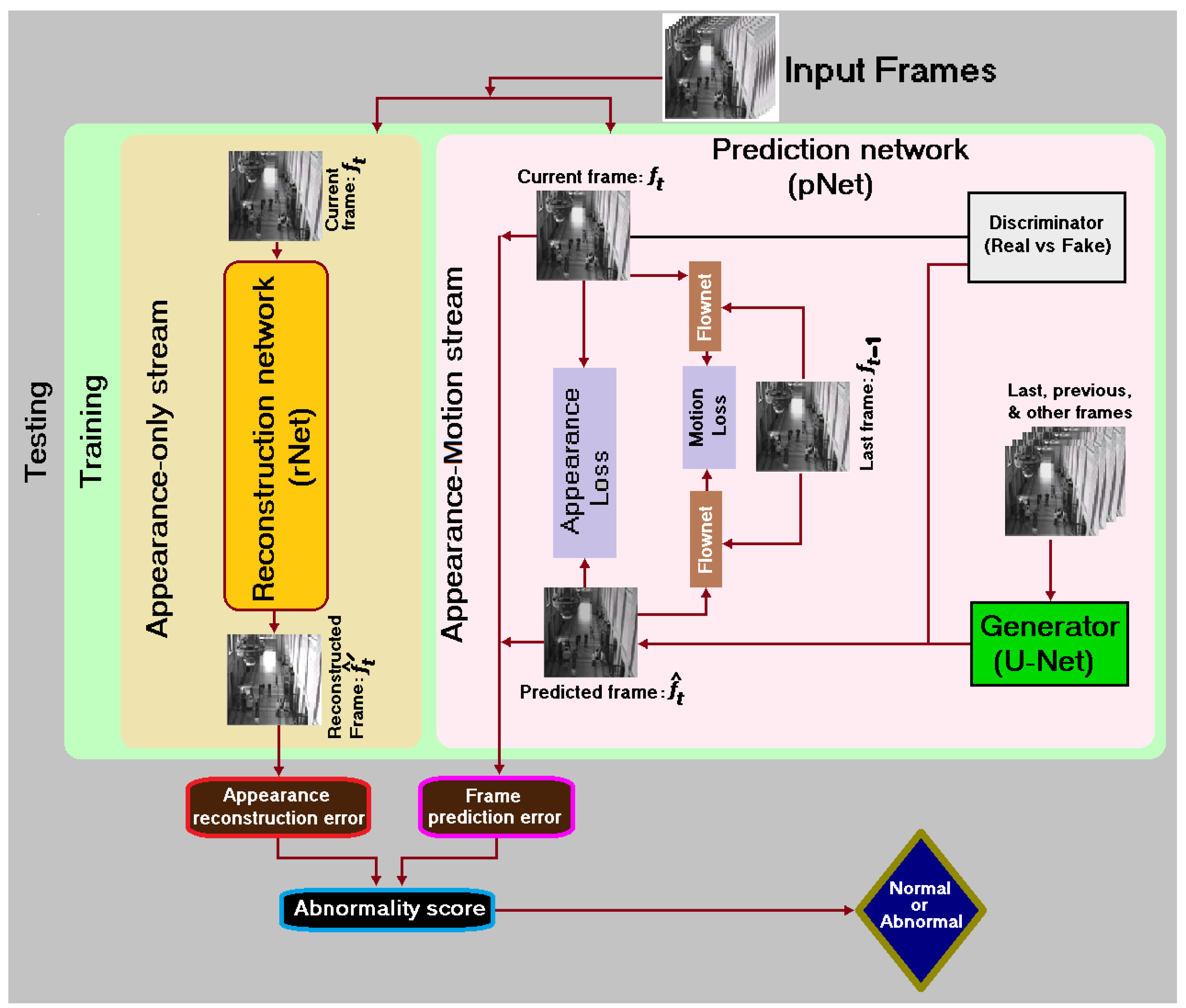
In this paper, we design a generalized architecture (rpNet) as shown in Figure 1, which includes a group of different deep models. Each model integrates an rNet (an image frame reconstruction network or an appearance-only stream) and a pNet (a video frame prediction network or an appearance-motion stream), in which every stream possesses its own contribution for the task of detecting abnormal frames. Both streams can promise substantial anomaly scores. The fusion of outputs from two streams guarantees a certain degree of augmentation of the error gap. Our approach is inspired by the Zhong et al. [3] model but with distinct modules and designs. Primarily, Zhong et al. [3] applied a traditional autoencoder (AE) as an rNet and the squeeze-and-excitation network of Hu et al. [8] as a pNet to handle motion. Differently, we apply a convolutional AE (ConvAE) or a skip connected ConvAE (AEc) as an rNet and we adopt Liu et al.’s [2] future frame prediction model as a pNet to handle appearance and motion. The performance of a ConvAE in rNet is better than a traditional AE. The ConvAE extends the basic structure of the simple AE by changing the fully connected layers to convolution layers. The ConvAE is more suitable for the images as it uses a convolution layer. The reason of choosing Liu et al. [2] prediction model is that a fixed and optimized procedure of optical flow estimation (e.g., FlowNet [9]) is embedded in it. Mainly, Liu et al. [2] applied a traditional U-Net [7] as the heart of their model. We also employ a traditional U-Net [7] as the first option of our pNet. Aside from a traditional U-Net [7], we propose to use two more of its derivatives, namely a non-local block U-Net and an attention block U-Net (aUnet), for performance improvements.

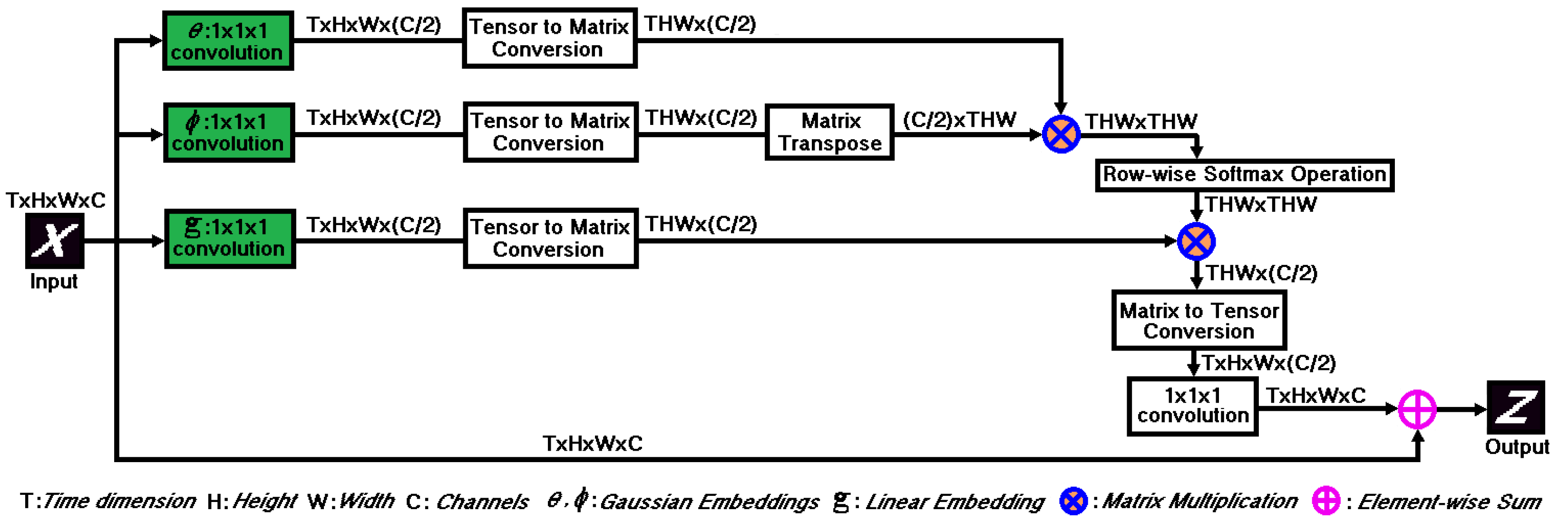
A U-Net [7] is an improved CNN (convolutional neural network) model that can train data with fewer samples and segment images more accurately, but its efficiency and effectiveness can be limited by using the local operators (e.g., convolutions and down-sampling operators) only [10]. However, non-local blocks can strengthen the temporal and spatial characteristics and establish the long-distance dependencies of video frames [11]. Buades et al. [12] explained non-local mean operation, and later Wang et al. [11] wrapped the non-local operation into a non-local block. A new non-local block can be inserted in a U-Net [7] without breaking its initial behavior [10]. Because of this, Zhang et al. 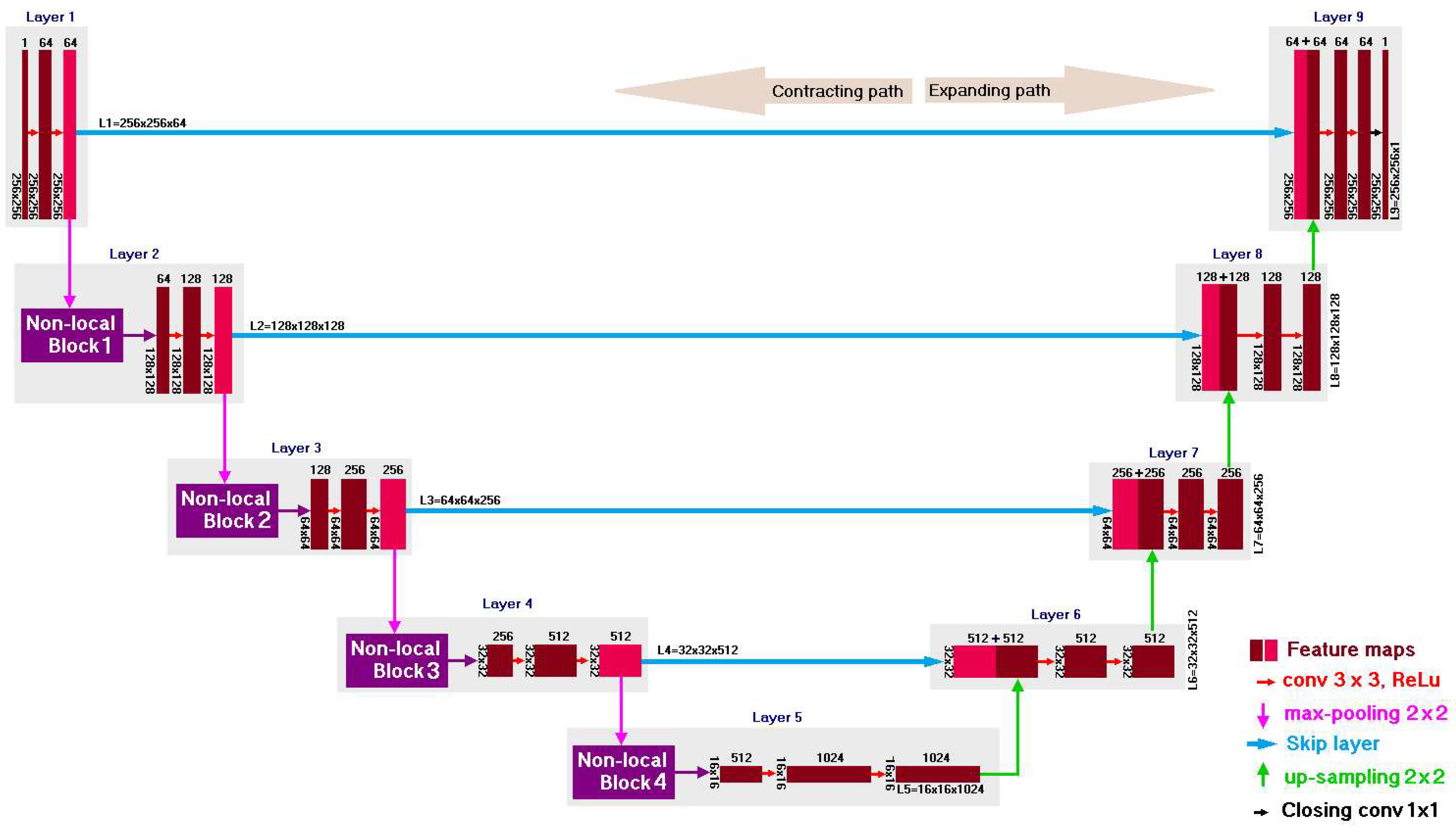[13] adopted three non-local blocks in their U-Net frame prediction model to detect surveillance video anomaly. However, Wang et al. 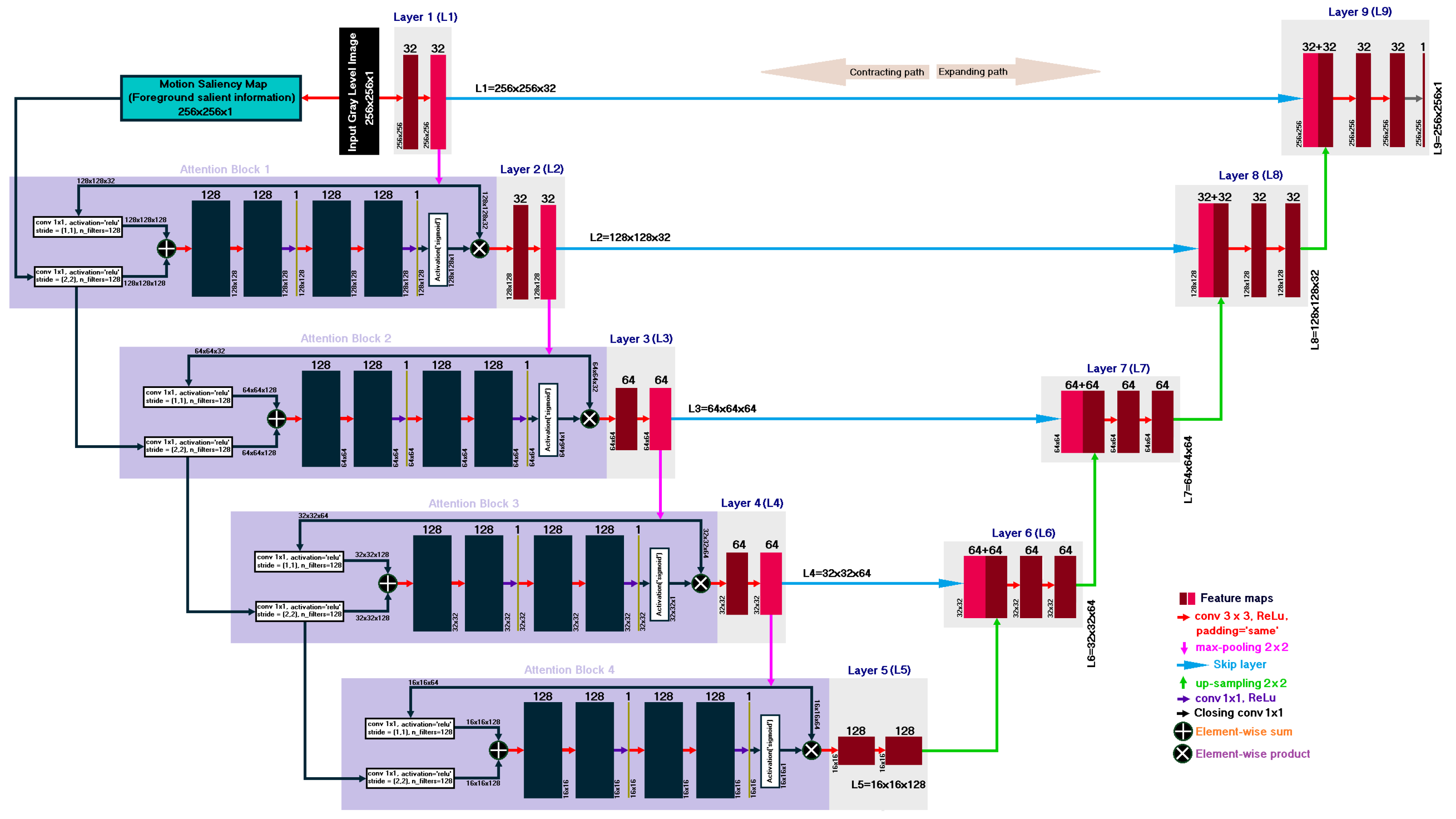[11] showed that more non-local blocks lead to better performance. To this end, we adopt four non-local blocks in the U-Net architecture as the second option of our pNet. In addition to non-local blocks, attention mechanism puts down less fitting features and highlights more salient features. Oktay et al. [14] introduced attention gates in the intermediate layers of a U-Net architecture for pancreas segmentation. Yet, due to better breast-tumor segmentation performance in ultrasound images, Vakanski et al. [15] applied attention blocks at beginning layers of a U-Net architecture. Following Vakanski et al. [15], we propose an aUnet as the third option of our pNet. There exist some internal architectural differences at our proposed aUnet from Vakanski et al. [15]. For example, Vakanski et al. [15] employed external auxiliary inputs in the form of visual saliency maps, whereas we employ an internal motion saliency map and original video frame as inputs of the aUnet.

We presume that if any frame $f_t$ contains an appearance anomaly then our rNet can improve its determinability, whereas if $f_t$ contains an appearance-motion anomaly, then our pNet can improve its determinability. The rNet and pNet enforce both the reconstructed frame and the predicted frame to be close to their ground truth frame, respectively. Therefore, we combine the error scores of both networks to calculate the final anomaly score of each frame for detecting its anomalousness by considering the anomaly scores of consecutive multi-frames (e.g., past, present, and future frames). This also helps to exploit the persistent flow of abnormal events. In essence, we propose six deep models by combining two-alternative of rNets and three-alternative of pNets from our generalized framework in Figure 1: (1) AE-Unet (convolutional autoencoder and U-Net), (2) AEcUnet (convolutional autoencoder with skip connection and U-Net), (3) AEnUnet (convolutional autoencoder and non-local block U-Net), (4) AEcnUnet (convolutional autoencoder with skip connection and non-local block U-Net), (5) AEaUnet (convolutional autoencoder and attention block U-Net), and (6) AEcaUnet (convolutional autoencoder with skip connection and attention block U-Net). Although these models can provide an improved error gap for abnormal events, they have different degrees of feature extraction capabilities required for crowd video anomaly detection. Consequently, in experimental setups, some of these models showed inferior results, while others presented superior results. For example, AEcaUnet demonstrated the best results and outperformed its alternatives by both confirming better error gap and extracting high quality features from the available videos.

Our key contributions are summarized as follows:

• We propose six different deep models for crowd anomaly detection by designing a generalized framework (rpNet).
• We propose an aUnet (see Figure 2) for an option of the pNet of our rpNet architecture.
• Experiments on five benchmark datasets and a rigorous statistical analysis demonstrate the potential of our models with competitive performance compared with the state-of-the-art models.

The rest of this paper is organized as follows. Section 2 addresses the most relevant previous studies. Section 3 overviews our generalized architecture of rpNet. Section 4 discusses the rNet of our rpNet. Section 5 illustrates the pNet of our rpNet. Section 6 exemplifies mainly the non-local block U-Net and our proposed aUnet. Section 7 illustrates anomaly detection on testing datasets. Section 8 hints a simulation to show that a larger error gap is guaranteed by rpNet. Section 9 explains experimental setup and results on publicly datasets. Section 10 compares our experimental results with the state-of-the-art methods. Section 11 makes a rigorous statistical analysis to find superiority among models. Section 12 concludes the paper.

2. Related Work

The related work can be classified into three groups, presented below.

2.1. Frame Reconstruction-Based Models

The following articles are primarily based on frame reconstruction and calculation of related errors. Xu et al. [16] proposed a multi-layer autoencoder (AE) for feature learning, which demonstrated the potency of deep learning features. Hasan  et al. [1] designed a three-dimensional convolutional autoencoder (ConvAE) for modeling regular frames. Chong et al. [17] took the advantages of both convolutional neural network (CNN) and recurrent neural network (RNN) for simultaneously modeling of the normal appearance and motion patterns. Luo et al. [18] proposed a temporally coherent sparse coding-based method, which can map to a stacked RNN framework. Sabokrou et al. [19] trained a generative adversarial network (GAN) similar to an adversarial network, in which a reconstruction component learned to reconstruct the normal test frames. However, all these reconstruction-based models assume that abnormal events can correspond to higher reconstruction errors, but this assumption may not necessarily hold always [2].

2.2. Frame Prediction-Based Models

The following studies mainly focus on how to predict future frames indirectly or directly. Shi et al. [20] modified the original long short-term memory (LSTM) along with a convolutional LSTM for precipitation forecasting. Mathieu et al. [6] proposed a multi-scale network with adversarial training for creating more natural future frames in videos. Giorno et al. [21] designed a deep model for detecting changes on a sequence of data from videos to see which frames were distinguishable from all the previous frames. By processing the video online Ionescu et al. [22] performed a similar work to that of Giorno et al. [21]. Lotter et al. [23] designed a deep predictive neural network for video prediction and unsupervised learning. Some studies (e.g., [24,25]) move to predict transformations required for creating future frames, which boosted the performance of video prediction to a greater extent. For example, Liu et al. [2] facilitated spatial and motion constraints for predicting future frame with normal events considering U-Net structure [7]. Their model also facilitated to detect those anomalies that do not agree the assumption. Their model was optimized according to the difference between the output and the original versions of video frame as well as the optical flow together with an adversarial loss. Doshi et al. [26] predicted the future video frame using previous video frames for video anomaly detection. To detect surveillance video anomaly, Zhang et al. [13] included the non-local block [11] in the U-Net [7] as a generator to generate high-quality prediction frames.

2.3. Reconstruction and Prediction-Based Models

The deep model of Nguyen et al. [27] consisted of three streams namely common encoder, appearance decoder, and motion decoder. Each stream had its own benefaction to detect exceptional frames. Basically, they combined a ConvAE for appearance along with a U-Net [7] for motion prediction. Their encoder was constructed by a sequence of blocks including convolution, batch-normalization, and leaky ReLU (rectified linear unit) activation. The decoder of their U-Net [7] had the same structure as the ConvAE except for the skip connections. Zhong et al. [3] proposed a cascaded model composed of a frame reconstruction network and an optical flow prediction network. By predicting optical flow based on reconstruction frame, their model increased the gap of prediction error of optical flow containing abnormal events.

The deep model of Liu et al. [28] composed of a prediction network, a reconstruction network, and a generative adversarial network (GAN). The prediction network integrated hybrid dilated convolution (HDC) [29] and DB-ConvLSTM [30] strategies to widen the gap between normal and abnormal events, while reconstruction network used an AE structure.

Inspired by the success of the video prediction model of Liu et al. [2], we adopt a U-Net structure to predict a frame from a number of recent ones and then estimate the corresponding optical flow. Similar to Liu et al. [2], a fixed procedure of optical flow estimation (e.g., FlowNet [9]) is embedded inside our pNet. The purpose of our rNet (i.e., ConvAE) is to learn the regular appearance structures.

Table 1. A qualitative comparison of the most related works. MSE: Mean Square Error, PSNR: Peak Signal to Noise Ratio.

Reference	Reconstruction	Prediction Network		Employed	Used Crowd Dataset
	Network	Generator	Optical Flow	Score
Liu et al. [2]	Not applicable	U-Net [7]	Flownet [9]	PSNR	Ped1 [31], Ped2 [18,31,32]
Nguyen et al. [27]	ConvAE	ConvAE + U-Net [7] with skip connections	FlowNet2 [33]	MSE	Ped2 [31,32], etc.
Zhong et al. [3]	Traditional AE	SE module [34]	Output of SE module [34]	MSE	Ped1 [31], Ped2 [18,31,32]
Liu et al. [28]	AE	U-Net [7] + HDC [29] + DB-ConvLSTM [30]	Difference of RGB [35]	PSNR	Ped1 [31], Ped2 [31,32]
Zhang et al. [13]	Not applicable	U-Net [7] + Non-local block [11]	Flownet [9]	PSNR	Ped1 [31], Ped2 [18,31,32]
AE-Unet (Ours)	ConvAE	U-Net [7]	Flownet [9]	PSNR	Ped1 [31], Ped2 [18,31,32,36]
AEcUnet (Ours)	ConvAE with skip connection	U-Net [7]	Flownet [9]	PSNR	Ped1 [31], Ped2 [18,31,32,36]
AEnUnet (Ours)	ConvAE	U-Net [7] + Non-local block [11]	Flownet [9]	PSNR	Ped1 [31], Ped2 [18,31,32,36]
AEcnUnet (Ours)	ConvAE with skip connection	U-Net [7] + Non-local block [11]	Flownet [9]	PSNR	Ped1 [31], Ped2 [18,31,32,36]
AEaUnet (Ours)	ConvAE	U-Net [7] + Proposed attention block + Proposed Motion Saliency Map	Flownet [9]	PSNR	Ped1 [31], Ped2 [18,31,32,36]
AEcaUnet (Ours)	ConvAE with skip connection	U-Net [7] + Proposed attention block + Proposed Motion Saliency Map	Flownet [9]	PSNR	Ped1 [31], Ped2 [18,31,32,36]

summaries a qualitative comparison of the most relevant works.

3. Overview of the Generalized Architecture (rpNet)

Fundamentally, we design a generalized architecture named rpNet as depicted in Figure 1. It consists of two neural networks connected in parallel namely reconstruction network (rNet) and prediction network (pNet). The rNet depends on appearance only as it works with images, but the pNet relies on both appearance and motion as it works with video frames. The key difference between images and video frames is that the video frames are sequential and correlated, whereas the images are static. Video frames need to be measured in both space and time dimensions, but images need to be measured in space dimension. The rpNet includes information of both images and video frames simultaneously.

Machine learning methods in computer vision and image processing problems [37] have been applied for a good deal of research applications (e.g., [38,39,40,41,42,43,44,45,46,47,48,49,50,51]). Deep learning is a subset of machine learning that utilizes huge volumes of data and sophisticated algorithms for training a model. Nowadays, deep learning models are used to detect anomalies in various kinds of applications (e.g., [52,53,54,55,56,57]). The extraction of appropriate features plays a decisive role for detecting anomalies in deep learning models. Recently, due to powerful capability of deep learning models in reconstruction, it has unquestionably made advancement in abnormal event detection tasks. The video anomaly detection models (e.g., [1,52]) indicated that convolution is predominantly applied for extracting features. Thereupon, such structure scarcely encodes temporal dependencies in a long video sequence. Basically, our rNet is a convolutional autoencoder, which is similar to those models [1,52]. 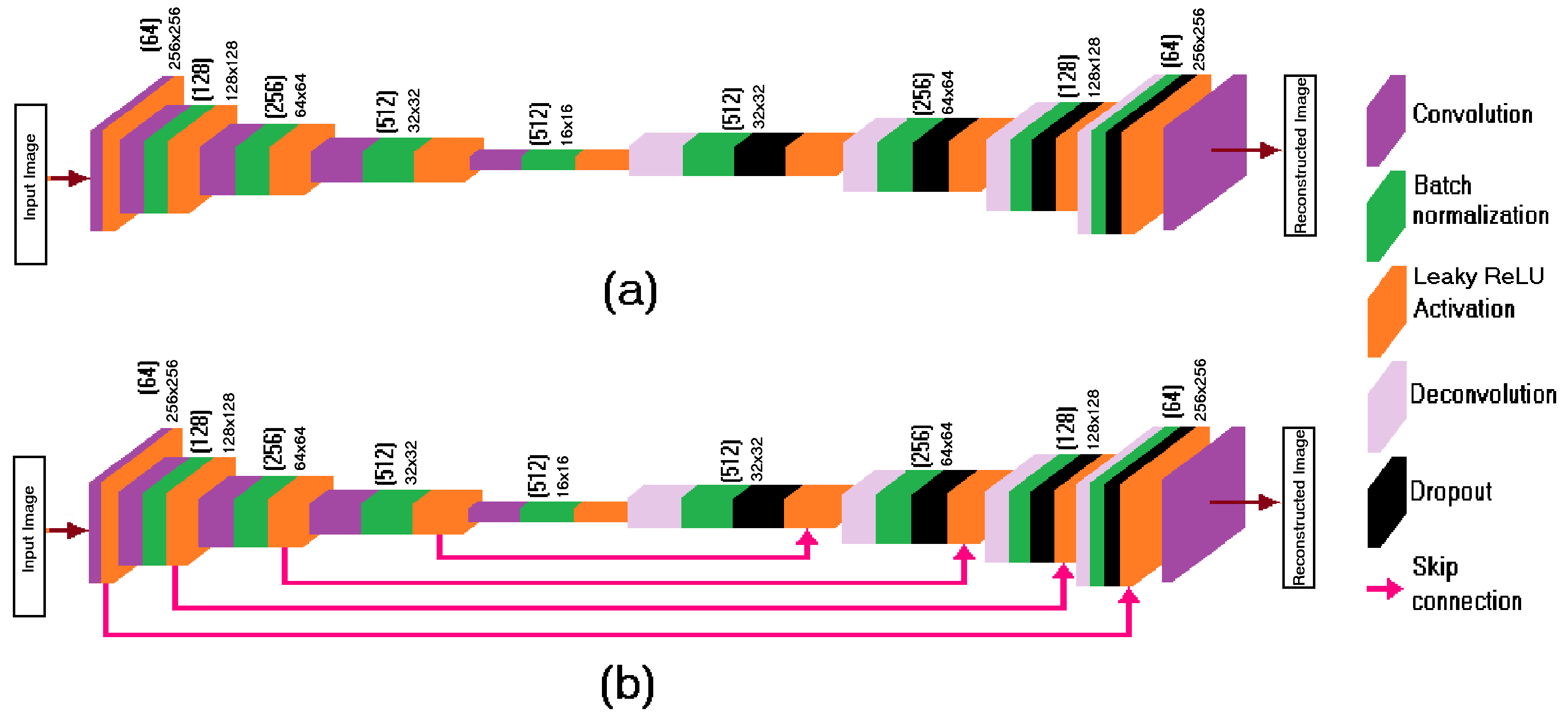Figure 3 details the two variants of the presented block diagram of the rNet in Figure 1. In general, the rNet comprises an encoding path and a decoding path. The block diagram of the pNet in Figure 1 is typically a prediction network of Liu et al. [2] to predict future frames. One of its most important components is its generator, which is a traditional U-Net [7]. However, we propose to use either non-local block U-Net or attention block U-Net as discussed in Section 6.

In a nutshell, the rpNet both reconstructs the current frame using its rNet for scoring reconstruction error and predicts the future frame using its pNet for scoring prediction error in a parallel manner for anomaly detection by providing better error gaps via information fusion (e.g., see Section 8). Both rNet and pNet can show some degree of performance, but the performance of rpNet is better than that of either rNet or pNet individually. The straightforward simulation in Section 8 and later the experimental results support this proposition. Essentially, the rpNet brings about six separate models namely AE-Unet, AEcUnet, AEnUnet, AEcnUnet, AEaUnet, and AEcaUnet by combining the two-variant of rNets and the three-variant of pNets.

Figure 3a demonstrates encoder and decoder networks of our ConvAE without skip connection. The encoder network consists in a stack of four hidden layers with convolutional filters of 64, 128, 256, and 512, kernel sizes of 5, 5, 3, and 3, and strides of (1,2), (2,2), (2,2), and (2,2), respectively. Regarding the decoder network, it has four transposed convolutional layers that mirror the encoder layers. Due to the loss of some features, the reconstructed image of ConvAE may not match exactly with the input image. The difference $L(f,\widehat{f^{\prime }})$ between the original input f and the reconstructed $\widehat{f^{\prime }}$ is called the reconstruction error. The learning process of ConvAE is to minimize the reconstruction error. Loss functions play an important role in achieving the desired reconstructed image.

4. Appearance-Only Stream

In this section, we discuss in detail our adopted two alternative reconstruction networks. A ConvAE is used to extract the salient features by performing filter operations on the original input image, whereas AEc boosts the performance with a notable margin.

4.1. ConvAE

The CNN has strong capability to learn spatial features [2]. Usually, a CNN consists of convolutional layer, activation layer, pooling layer, and up-sampling layer. It uses these layers to extract features from the two-dimensional (2D) data structure of images and then followed by the sub-sampling or pooling layer. We can add a dense or feedforward layer to the CNN for classification tasks, or we can add an upsampling layer to increase the resolution of the feature maps for image generation tasks. Activation layers consist of activation functions (e.g., ReLU, Sigmoid, Softmax, Tanh, and Linear), which introduce non-linearity into the deep neural network. Without this non-linearity, the deep neural networks are only able to perform the linear mapping between inputs and the outputs. The pooling or sub-sampling layers can reduce the spatial dimensions of the feature maps (e.g., from 256 × 256 to 128 × 128). Theoretically, we can eliminate the down/up sampling layers altogether. The up-sampling layer performs the reverse of the pooling layer. It is used to increase the dimensions of the incoming feature maps (e.g., from 128 × 128 to 256 × 256). The up-sampling layer is generally used in generative tasks. Leaky ReLU decreases certain positive values to 0 if they are close enough to zero. In dropout technique, randomly selected neurons are ignored during training. A good value for dropout in a hidden layer is between 0.50 and 0.80.

The AE is primarily used for image reconstruction. The AE that employs CNN mimics its input to its output as close as possible. It aims to take an input, transform it into a reduced representation called code or embedding. Then, this code or embedding is transformed back into the original input. The code is also called the latent-space representation. An AE consists of two leading parts namely an encoder and a decoder. Stacking encoders and decoders with multiple hidden layers can form a deep autoencoder. The encoder extracts features by gradually reducing the spatial resolution, whereas the decoder gradually recovers the frame by increasing the spatial resolution. The encoder maps the input into the code, whereas the decoder maps the code to a reconstruction of the input. Fully connected AE ignores 2D image structure [58]. The ConvAE extends the basic structure of the simple AE by changing the fully connected layers to convolution layers. The ConvAE is very suited for the images as it uses a convolution layer. The convolutional layers are excellent for extracting features from the images or other 2D data without modifying (reshaping) their structure. An encoder can employ convolutional layer, batch normalization layer, an activation function, and a max-pooling function for reducing the dimensions of the feature maps. After a specific number of layers, when the encoder is complete, the feature maps are flattened and a dense layer is used for the latent-space representation. The deconvolution is used for the up-sampling of the incoming feature maps, which is usually followed by the batch normalization and the activation function. Kernel size is one of important parameters in CNN. The smaller the size of kernel, the more effective the preserving details of the original image and the lower the computational cost of network. However, the extreme kernel size of $1\times 1$ extracts local information from an image without considering spatial relationship of pixel. Therefore, we can set the size of kernel to 5 and 3 for both considering the spatial relationship of pixel and reducing computational cost.

4.2. Loss Function

The performance of ConvAE depends on input data and the loss function. The goal of training is to minimize the loss. When the main goal of the ConvAE is to solely reconstruct the input as accurate as possible, the loss function of MSE or Kullback–Leibler (KL) divergence [59] can be used. The intensity loss $L_{in{t}_r}$ of the reconstruction network can be calculated by Equation (1) on minimizing the distance measured by $l_2$-norm between $\widehat{f_t^{\prime }}$ and $f_t$ as:

$$L_{in{t}_r}(\widehat{f_t^{\prime }},f_t)=\left|\right|\widehat{f_t^{\prime }}-f_t{\left|\right|}_2^2.$$

(1)

The gradient loss $L_{g{d}_r}$ of reconstruction network can be calculated by Equation (2) as:

$$L_{g{d}_r}(\widehat{f_t^{\prime }},f_t)=\sum _{i,j}\Vert |{\widehat{f_t^{\prime }}}_{i,j}-{\widehat{f_t^{\prime }}}_{i-1,j}|-|{f_t}_{i,j}-{f_t}_{i-1,j}{|\Vert }_1+\Vert |{\widehat{f_t^{\prime }}}_{i,j}-{\widehat{f_t^{\prime }}}_{i,j-1}|-|{f_t}_{i,j}-{f_t}_{i,j-1}{|\Vert }_1.$$

(2)

4.3. Replacing ConvAE by AEc

If ConvAE goes deeper or applying operations including max pooling, it cannot work very well even with deconvolution layers. A performance degradation problem is encountered when deeper networks start converging [60]. This is possibly due to the fact that a big amount of image details could be lost or corrupted during the convolution and the pooling. This drawback saturates the performance of the network as the depth of network expands. Specially, if the ConvAE encounters this type of problem, it is arduous to learn the details from the data. To minimize this problem, inspired by He et al. [60], we add skip connections between two corresponding convolutional and deconvolutional layers as shown in Figure 3b. The response from a convolutional layer is directly propagated to the corresponding mirrored deconvolutional layer, both forwardly and backwardly. The skip connections between the corresponding encoder and decoder layers allows the network to converge to a better optimum in pixel-wise prediction problems [61]. Let the outputs from the encoder layer and the corresponding decoder layer be $Ou{t}_{e{l}_i}$ and $Ou{t}_{d{l}_i}$, respectively. The input to the next decoder layer $I{n}_{d{l}_{i+1}}$ is calculated by Equation (3) as:

$$I{n}_{{dl}_{i+1}}=Ou{t}_{{el}_i}\oplus Ou{t}_{{dl}_i}.$$

(3)

Each skip connection complements the data loss due to the data compression in the encoder part by combining the encoder convolutional layer output and the up-sampling output. Through skip connections, each feature map of the corresponding encoder and decoder are summed element-wise, which helps the network to recover the image well.

5. Appearance-Motion Stream

In this section, we discuss details of our prediction network and summarize the loss functions for optimization.

Only appearance constraints cannot guarantee to characterize the motion information well. Further, both spatial and temporal information is an important feature of videos. Inspired by Liu et al. [2], we used an optical flow constraint into the objective function to guarantee the motion consistency for normal events in training set, which further boosts the performance for anomaly detection. The pipeline of our video frame prediction network is shown in Figure 1, where we adopt a traditional U-Net [7] as generator to predict next frame. The traditional U-Net [7] is a fully convolutional neural network, and it uses convolutional and pooling layers. To reduce the number of parameters, it does not have any fully connected layer. It contains a contraction path and an expansion path. Its contraction path is employed to extract the features through the convolutional layer and downsampling. Its expansion path accurately locates and restores the information as much as possible. There is also a shortcut operation before each upsampling convolutional layer to concatenate the information.

To generate high quality image, we adopt the constraints in terms of appearance (e.g., intensity and gradient) as well as motion (e.g., optical flow) losses. Optical flow is a widely used estimator of motion. The Flownet [9] is a pre-trained network used to calculate optical flow. We also clenched the adversarial training to discriminate whether the prediction is real or fake. The aim of our appearance-motion stream is not only to predict frames to be close to their ground truth in spatial space but also to match the optical flow between predicted frames and the ground truth. In common, this stream is expected to associate typical motions to common appearance objects while ignoring the static background patterns.

Given a video with consecutive t frames as $\{f_1,f_2,\dots ,f_t\}$. We predict the future video frame $\widehat{f_t}$ using previous video frames $\{f_1,f_2,\dots ,f_{t-1}\}$. Following the work by Mathieu et al. [6], to make the predicted $\widehat{f_t}$ close to its ground truth $f_t$, we minimize their distances with reference to intensity and gradient. Following the work of Liu et al. [2], to preserve the temporal coherence between neighboring frames, we enforce the optical flow between $f_t$ and $f_{t-1}$ as well as the optical flow between $\widehat{f_t}$ and $f_{t-1}$ to be close. We assume that normal events can be predicted very well. Therefore, we can include the difference between the predicted frame $\widehat{f_t}$ and its ground truth $f_t$ for anomaly detection score. Following the work by Liu et al. [2], we employ a traditional U-Net [7], which serves as the main prediction network for a shortcut between a high-level layer and a low-level layer with the output resolution unchanged for each two convolution layers to decrease gradient vanishing and to increase information symmetry. The kernel sizes are configured to all convolution and deconvolution as $3\times 3$, and the max pooling layers as $2\times 2$.

5.1. Appearance Loss

To make the prediction close to its ground truth, following the work of Mathieu et al. [6], intensity and gradient difference can be employed.

5.1.1. Intensity Loss

Intensity loss is the $l_1$-norm or $l_2$-norm between the predicted frame $\widehat{f_t}$ and its ground true $f_t$, which is used to maintain similarity between pixels in the RGB space. By definition, the sum of the absolute values is the $l_1$-norm, and the sum of squared values is the $l_2$-norm. While the $l_1$-norm increases at a constant rate, the $l_2$-norm increases exponentially. Minimization of the norm encourages the weights to be small. Specifically, we minimize the distance measured by $l_2$-norm between $\widehat{f_t}$ and $f_t$ as intensity loss $L_{in{t}_p}$ of the prediction network by Equation (4) [2]:

$$L_{in{t}_p}(\widehat{f_t},f_t)=\left|\right|\widehat{f_t}-f_t{\left|\right|}_2^2.$$

(4)

5.1.2. Gradient Loss

There exists a flaw in calculating pixel intensity loss by $l_2$-norm, which produces blur in the output. Henceforth, it is vital to apply gradient difference loss for sharpening the predicted frame $\widehat{f_t}$ by using the $l_1$-norm. As compared to $l_2$-norm, $l_2$-norm is more likely to reduce some weights to 0. The gradient loss $L_{g{d}_p}$ of the prediction network can be calculated by Equation (5) as:

$$L_{g{d}_p}(\widehat{f_t},f_t)=\sum _{i,j}\Vert |{\widehat{f_t}}_{i,j}-{\widehat{f_t}}_{i-1,j}|-|{f_t}_{i,j}-{f_t}_{i-1,j}{|\Vert }_1+\Vert |{\widehat{f_t}}_{i,j}-{\widehat{f_t}}_{i,j-1}|-|{f_t}_{i,j}-{f_t}_{i,j-1}{|\Vert }_1,$$

(5)

where ${f_t}_{i,j}$ denotes the pixel at the i-th row and j-th column in $f_t$, and $|.|$ returns the absolute value.

5.1.3. Motion Loss

To detect anomaly the coherence of motion is an important factor for the evaluation of normal events. Only difference between intensity and gradient for future frame generation cannot guarantee to predict a frame with the correct motion. Optical flow is a good estimator of motion [62]. We adopt a temporal loss defined as the difference between optical flow of predicted frames and ground truth to improve the coherence of motion in the predicted frame. We employ the Flownet [9] denoted as F, which is a CNN-based approach for optical flow estimation. We consider that F is pre-trained on a synthesized dataset [9] and all the parameters in F are fixed. The motion loss $L_{mot}$ in terms of optical flow can be measured by $l_1$-norm using Equation (6) as:

$$L_{mot}({\widehat{f}}_t,f_t,f_{t-1})=\left|\right|F({\widehat{f}}_t,f_{t-1})-F(f_t,f_{t-1}){\left|\right|}_1.$$

(6)

5.1.4. Adversarial Generator Loss

Usually, a generative adversarial network (GAN) contains a generator G and a discriminator D. The G learns to generate frames that are hard to be classified by D. Similar to Liu et al. [2], we use a U-Net-based prediction network as G. As for D, we follow Isola et al. [63] and utilize a patch discriminator, which means each output scalar of D corresponds a patch of an input image. The goal of training D is to classify $f_t$ into class 1 (i.e., genuine label) and $G(f_1,f_2,\dots ,f_{t-1})=$${\widehat{f}}_t$ into class 0 (i.e., fake label), respectively. The goal of training G is to generate frames, whereas D classify them into class 1. The adversarial generator loss $L_{adg}$ is minimized to confuse D as much as possible such that it cannot discriminate the generated predictions, and is given by the MSE loss function as:

$$L_{adg}\left(\widehat{f_t}\right)=\sum _{i,j}\frac{1}{2}{L}_{MSE}(D\left({\widehat{f_t}}_{i,j}\right),1),$$

(7)

where $D\left(f_{i,j}\right)=1$ denotes real decision by D for patch $(i,j)$, $D\left({\widehat{f_t}}_{i,j}\right)=0$ indicates fake decision, and $L_{MSE}$ is the mean squared error function.

5.2. Minimization Objective Function

We combine the losses on appearance, motion, and adversarial training to obtain the following minimization objective function:

$$\begin{array}{cc}\hfill & L(f_t,f_{t-1},{\widehat{f}}_t,{\widehat{f^{\prime }}}_t)={\lambda }_{in{t}_p}{L}_{in{t}_p}(\widehat{f_t},f_t)+{\lambda }_{g{d}_p}{L}_{g{d}_p}(\widehat{f_t},f_t)+{\lambda }_{in{t}_r}{L}_{in{t}_r}(\widehat{f_t^{\prime }},f_t)\hfill \\ \hfill & +{\lambda }_{g{d}_r}{L}_{g{d}_r}(\widehat{f_t^{\prime }},f_t)+{\lambda }_{mot}{L}_{mot}({\widehat{f}}_t,f_t,f_{t-1})+{\lambda }_{adg}{L}_{adg}\left(\widehat{f_t}\right),\hfill \end{array}$$

(8)

where ${\lambda }_{in{t}_p}$, ${\lambda }_{g{d}_p}$, ${\lambda }_{in{t}_r}$, ${\lambda }_{g{d}_r}$, ${\lambda }_{mot}$, and ${\lambda }_{adg}$ are the corresponding training time weights for the losses. To train the model, the intensity of pixels in all frames can be normalized (e.g., [−1, 1]). An Adam [64]-based stochastic gradient descent method can be used for parameter optimization.

6. Replacement of Traditional U-Net

In this section, we discuss two alternative replacements of basic U-Net.

6.1. Replacing Basic U-Net by Non-Local Block U-Net

The non-local mean value at a given pixel is the weighted average of all pixels in an image, but the kind of weights depend on the likeness between pixels, i.e., similar pixel neighborhoods have bigger weights. For example, considering Figure 4, to calculate the non-local mean at a pixel in Region 1, due to the similarity, the pixels in Region 4 and Region 9 obtain larger weights compared with the rest of seven regions. Similarly, for Region 3, the pixels in Region 5 and Region 10 obtain larger weights than those in the rest of the seven regions, and so on. Thus non-local mean preserves long distance dependence as indicated by arrows.

Buades et al. [12] explained non-local mean operation. Wang et al. [11] proposed a generic non-local operation as:

$$y_i=\frac{1}{\mathcal{C}\left(x\right)}\sum _{{\forall }_j}f(x_i,x_j)g\left(x_j\right),$$

(9)

where x and y denote the input and output signals, respectively. Here, i and j indicate the index of an output position in space-time and the index of enumerating all possible positions, respectively. The pairwise function f determines the scalar between i and all j, while the unary function g computes a representation of the input signal at j. In the end, y is obtained following a normalization by the factor of $\mathcal{C}\left(x\right)$.

Wang et al. [11] also wrapped the non-local operation shown in Equation (9) into a non-local block that can be embedded in many existing pre-trained networks including U-Net [7] without affecting its standard behavior. Unlike fully connected layers that are frequently used at the end, a non-local block can be added into the earlier part of deep neural networks—resulting a combination of both local and non-local information in an ample hierarchy. A non-local block can be defined by Equation (10) as [11]:

$$z_i=W_z{y}_j+x_i,$$

(10)

where $W_z$ belongs to a weight matrix and “+” denotes a residual connection.

Figure 5 depicts a space-time non-local block [11] with the embedded Gaussian. The input feature maps are presented as their tensors with the shape of $T\times H\times W\times C$, i.e., the input dimension of X is $T\times H\times W\times C$. The green colored boxes indicate $1\times 1\times 1$ convolution. This space-time non-local block is similar to the block in the architecture of ResNet [60]. So, the non-local operation can be easily inserted into the existing network structure. However, the convolution is performed using a convolution kernel with a size of $1\times 1\times 1$ to obtain the outputs of three branches ($\theta$, $\phi$, and $\mathbf{g}$) with the dimension of $T\times H\times W\times (C/2)$. Afterwards, three outputs of these branches with dimension of $THW\times (C/2)$ are obtained through tensor to matrix conversion process. The output of the $\phi$ branch is transposed, and then this output and the output of the $\theta$ branch are multiplied using matrix multiplication rule to obtain the output dimension of $THW\times THW$. Subsequently, the SoftMax operation is performed on each row. Later, the matrix multiplication with the output of the $\mathbf{g}$ branch is performed to obtain the output dimension of $THW\times (C/2)$. A reshaping of $THW\times (C/2)$ is carried out through matrix to tensor conversion process for getting the output dimension of $T\times H\times W\times (C/2)$. The output dimension of $T\times H\times W\times C$ from the $1\times 1\times 1$ convolution layer and the original input dimension of $T\times H\times W\times C$ perform element-wise summation to achieve the final output Z. This element-wise summation is similar to the residual connection in the ResNet [60]. Two optimization techniques are applied to improve the computational efficiency of the non-local block: (1) The number of convolution kernels for $\theta$, $\phi$, and $\mathbf{g}$ operations is set to the half of the number of input feature map channels (i.e., $C/2$); (2) The pooling method is applied to sample the output of $\theta$, $\phi$, and $\mathbf{g}$, so that the size of the feature map output is reduced to half of the original.

Similar to the traditional U-Net [7], the non-local block U-Net contains both contracting and expanding paths. There are some advantages to use non-local block in the U-Net [7] including the non-local operations that can directly capture remote dependencies and can also improve the correlation of distant pixels for gaining a richer feature map. However, the usage of non-local block in U-Net [7] for detecting video anomaly is not new. For example, Zhang et al. [13] used three non-local blocks in their U-Net frame prediction model for detecting surveillance video anomaly. Nevertheless, Wang et al. [11] suggested that more non-local blocks lead to better results. To this end, we propose to employ four non-local blocks in the U-Net architecture for our prediction network. Figure 6 shows our adopted non-local block U-Net. Basically, it consists of a traditional U-Net [7] and four non-local blocks. Those non-local blocks are added in downsampling. On the whole, the contracting path of our non-local U-Net extracts features through the convolutional layer and downsampling; while the expanding path precisely pinpoints and restores the information to the greatest extent. There are also skip layers to fuse the information. In the contracting path, $3\times 3$ convolution followed by ReLU activation and $2\times 2$ maximum pooling layers are applied. A $2\times 2$ maximum pooling layer is added after every two convolutional layers (e.g., the $2\times 2$ maximum pooling layer between Layer 1 and Layer 2). Every step of upsampling in the expanding path bridges to the contracting path for fabricating high-quality images.

6.2. Replacing Basic U-Net by aUnet

Attention mechanism contributes to suppress less relevant features and emphasizing more important features in image classification. Commonly, attention in deep neural networks is mainly implemented in two forms, namely, hard (or stochastic) attention and soft (or deterministic) attention. The implementation of hard attention is non-differentiable [65], whereas soft attention models are differentiable [66]. Thus, the soft attention is a preferable form of implementation. Roughly, there exist two types of soft-attention-based models: (i) Usage of intermediate layers of the architecture, and (ii) Usage of beginning layers of the architecture. For example, for image classification, Jetley et al. [67] introduced attention gates at three intermediate layers in a VGG network and a weighted combination of the attention maps was employed in the last layer. Oktay et al. [14] introduced attention gates in a U-Net architecture for segmentation of the pancreas. In both models, the attention blocks employ activation maps from the intermediate layers in the model as saliency maps for enhancing the discriminative characteristics of extracted intermediary features. However, Vakanski et al. [15] claimed that the segmentation performance would not be improved using the self-attention blocks described in Jetley et al. [67] and Oktay et al. [14]. Thus, they applied the attention blocks at beginning layers of their architecture for breast tumor segmentation in ultrasound images. Basically, their proposed attention block utilized pre-computed saliency maps that specified to target spatial regions.

Our design of the attention blocks in U-Net was inspired by the attention blocks of Vakanski et al. [15]. Differently from their network, our proposed attention blocks in this work utilizes motion saliency maps that point out to target salient regions of motion. Further, there are some internal architectural differences. For example, the pre-computed input spatial salient map of Vakanski et al. [15] is down-sampled through a max-pooling layer following the standard Equation (11) as:

$$\beta =⌊\frac{\gamma -\kappa +2\rho }{s}⌋+1,$$

(11)

where $\gamma$, $\beta$, $\kappa$, $\rho$, and s indicate number of input features, the number of output features, convolution kernel size, convolution padding size, and convolution stride size, respectively. We also follow Equation (11), but our instantaneously computed motion saliency map is down-sampled through a $1\times 1$ convolution followed by ReLU activation and $2\times 2$ stride operation. A graphical representation of our proposed aU-Net is presented in Figure 2.

6.2.1. Operation of the aUnet

Essentially, our proposed aU-Net in Figure 2 consists of a standard U-Net, a motion saliency map, and $\tau$ number of attention blocks with $\tau \in \{1,2,3,4\}$. The discussion of motion saliency map covers in the next subsection. However, the input feature map is down-sampled through a $2\times 2$ max-pooling layer and then fed to the attention block. The motion saliency map is fed to the $\tau$th attention block with horizontal and vertical spatial dimensions of $256/2^{\tau -1}\times 256/2^{\tau -1}$ pixels. This feeding is performed directly for the first attention block, but for other attention blocks indirectly via their preceding attention blocks. At the $\tau$th attention block, the motion saliency map with horizontal and vertical spatial dimensions of $256/2^{\tau -1}\times 256/2^{\tau -1}$ pixels is passed through $1\times 1$ convolution layer followed by ReLU activation, $2\times 2$ stride layer, and 128 number of filters. After $2\times 2$ max-pooling, the input feature map at the $\tau$th attention block with horizontal and vertical spatial dimensions of $256/2^{\tau }\times 256/2^{\tau }$ pixels is also passed through $1\times 1$ convolution layer followed by ReLU activation, $2\times 2$ stride layer, and 128 number of filters. The spatial dimensions of both input feature map with size of $256/2^{\tau }\times 256/2^{\tau }\times 128$ and the motion saliency map with size of $256/2^{\tau }\times 256/2^{\tau }\times 128$ match, and then they perform a summation at an element-wise sum block. Its output is an intermediate feature map with size of $256/2^{\tau }\times 256/2^{\tau }\times 128$. This map is further refined through a series of linear $3\times 3\times 128$ and $1\times 1\times$ convolution layers followed by ReLU activation. A sigmoid activation function normalizes the values into the range of $[0,1]$ and outputs a semi-attention map with a spatial size of $256/2^{\tau }\times 256/2^{\tau }\times 1$. This semi-attention map with size of $256/2^{\tau }\times 256/2^{\tau }\times 1$ and the max-pooled feature map with size of $256/2^{\tau }\times 256/2^{\tau }\times \varsigma$ perform a multiplication at an element-wise product block, where $\varsigma =32$ and $\varsigma =64$ for the first-second and third-fourth attention blocks, respectively. Its output is an attention map with size of $256/2^{\tau }\times 256/2^{\tau }\times \varsigma$, which is propagated to the next layer of the standard U-Net for further processing.

6.2.2. Motion Saliency Map

Normally, the human vision system pays more attention to the moving objects than the static regions. For this reason, motion becomes one of the key features of the visual attention model. Due to the elapse of time, an attention region on a frame becomes inattention region. We can define such phenomenon using a decay attention factor $deAtt$ with $1\le deAtt\le 255$ as:

$$\varpi =⌊\frac{255}{deAtt}⌋,$$

(12)

where $\varpi$ indicates the number of attention frames for a region (i.e., $\varpi$ frames later an attention region becomes a background region). For example, all current motion regions are paying maximum attention, but with $deAtt=60$ all such regions become zero attention regions after $\varpi =\lfloor 255/60\rfloor =4$ frames. Normally, it is not important to process all the regions in a frame. To speedup computation, we can obtain a region of interest (RoI) obtained by a motion heat map [68,69,70,71,72] to apply on the calculation of motion saliency map. Figure 7 indicates a straightforward RoI.

6.2.3. Algorithm

Algorithm 1 gives details of our motion saliency map creation algorithm. It assumes the foreground information of the current frame as the most salient feature.

Algorithm 1: Creation of Motion Saliency Map

Based on $deAtt$ values, the motion saliency map typically comprises of multiple attention maps with different resolutions, thereby capturing salient features across multiple levels of feature abstraction. Figure 8 shows some sample camera view frames from UCSD-Ped2 [31] dataset. Figure 9 shows two samples output of Algorithm 1 considering frames in Figure 8 and $deAtt=60$.

7. Anomaly Detection on Testing Data

If we assume that normal events can be well predicted, then we can easily apply the difference between the predicted frame $\widehat{f_t}$ and its ground truth $f_t$ for anomaly prediction. In anomaly detection methods, two common metrics, namely MSE and PSNR, are widely employed to calculate the anomaly scores. The MSE is used to measure the quality of predicted images by computing a Euclidean distance between the prediction and its ground truth of all pixels, whereas the PSNR represents a measure of the peak error. The MSE is easy to compute, but sensitive to outliers. On the other hand, in the absence of error, if two images $f_t$ and $\widehat{f_t}$ (or $\widehat{f_t^{\prime }}$) are identical, then the MSE is zero but the PSNR becomes infinite (or division by zero) [73]. In spite of that, Mathieu et al. [6] showed that PSNR is a better way for image quality assessment.

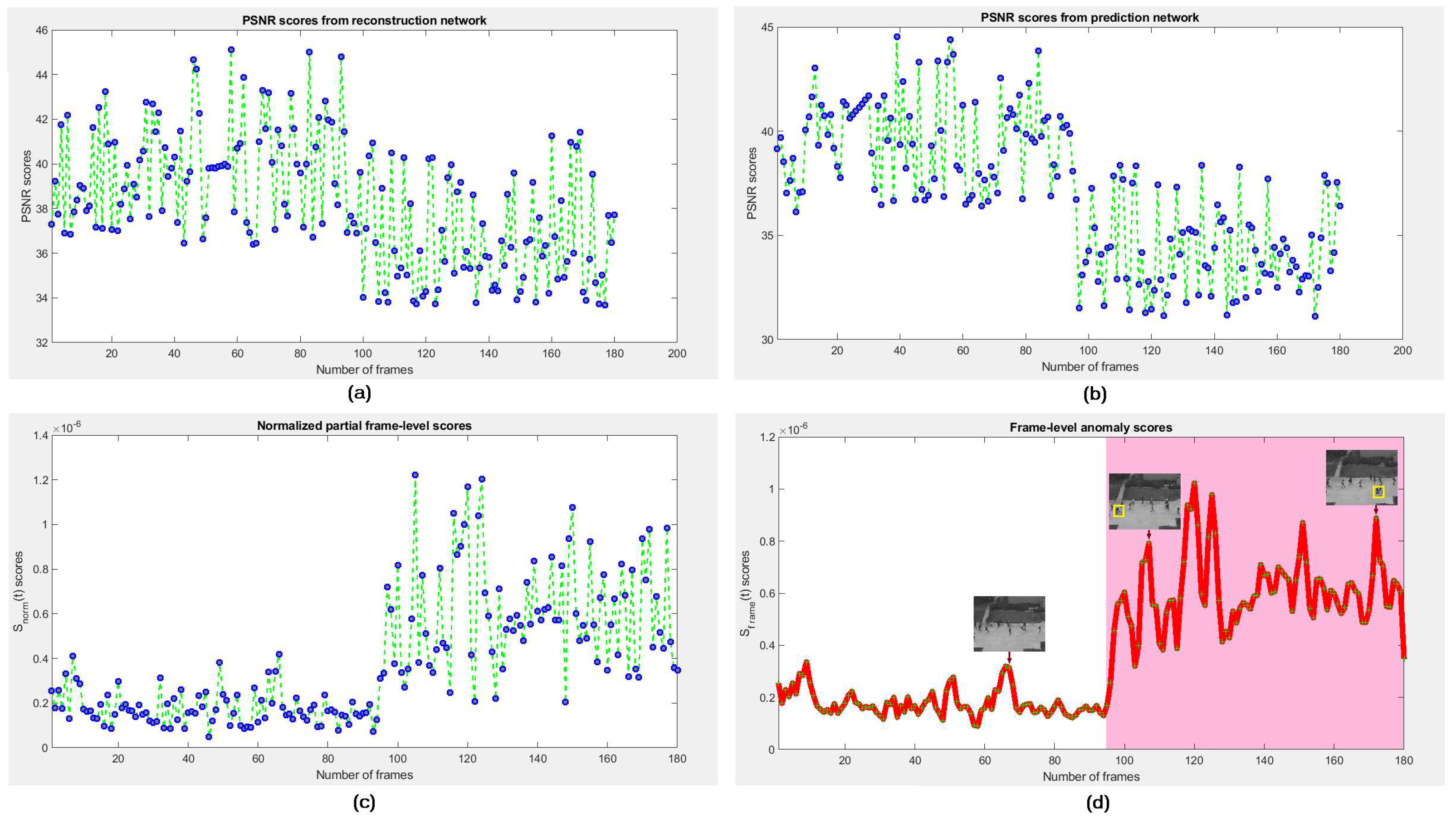
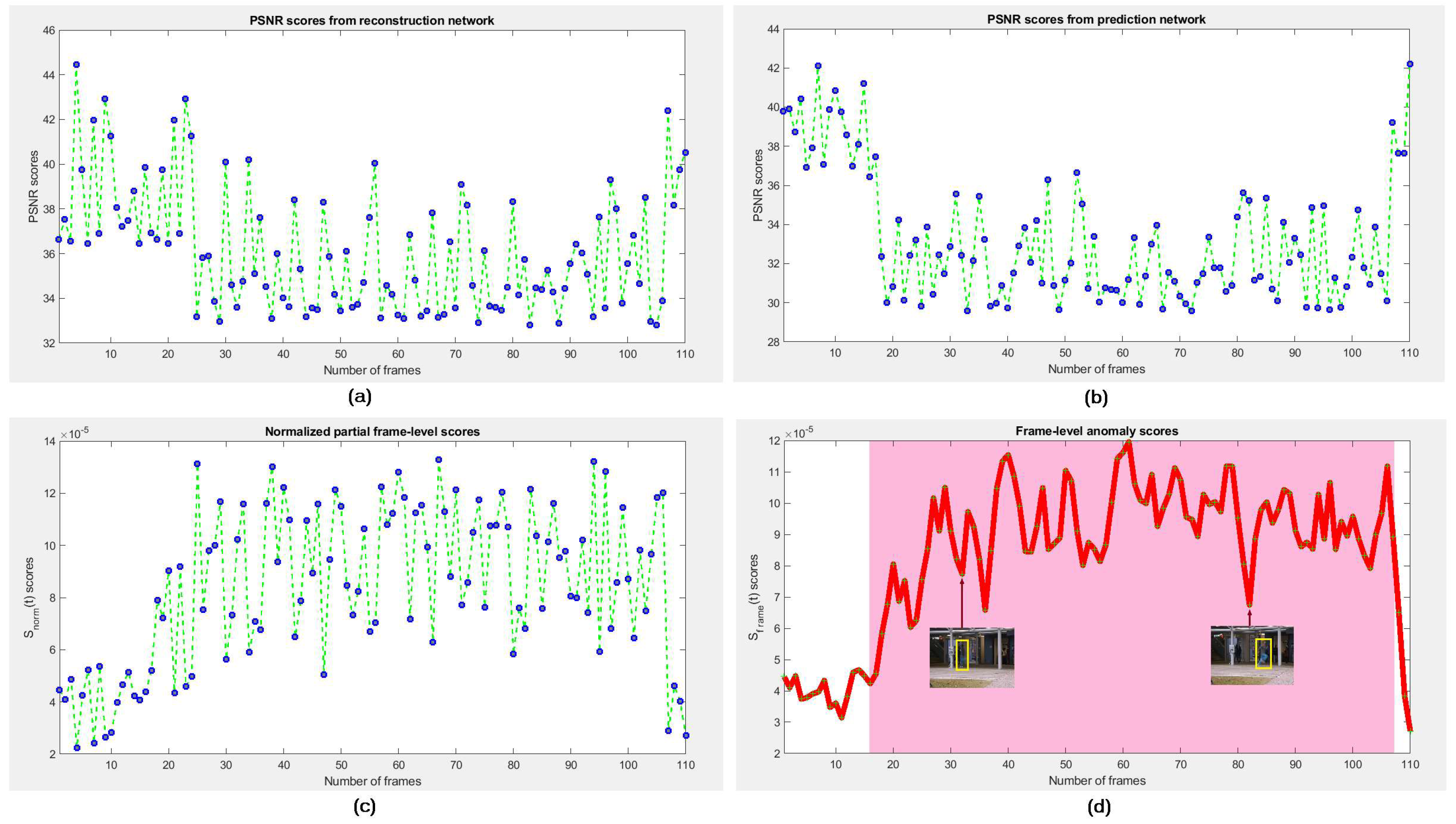
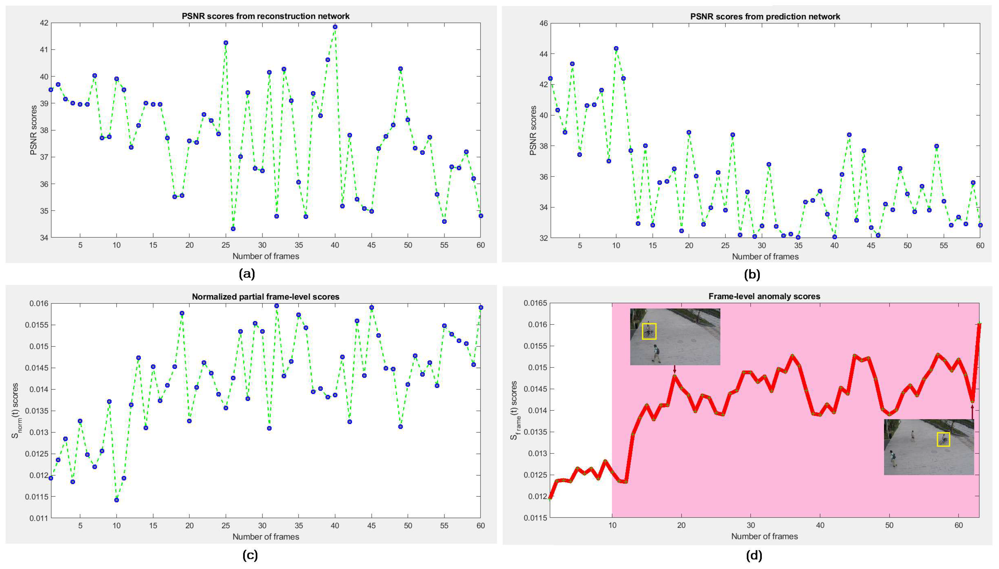
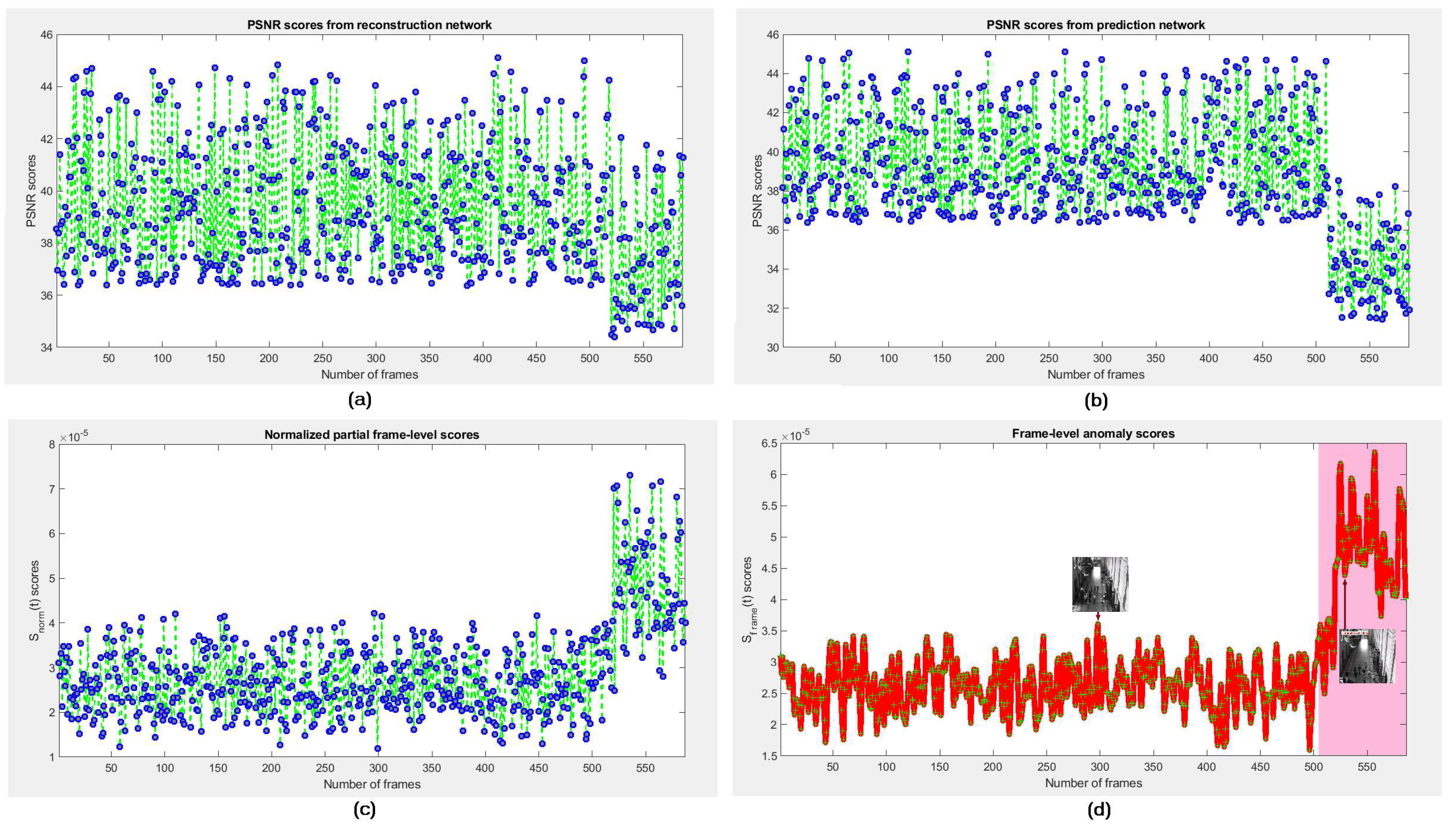
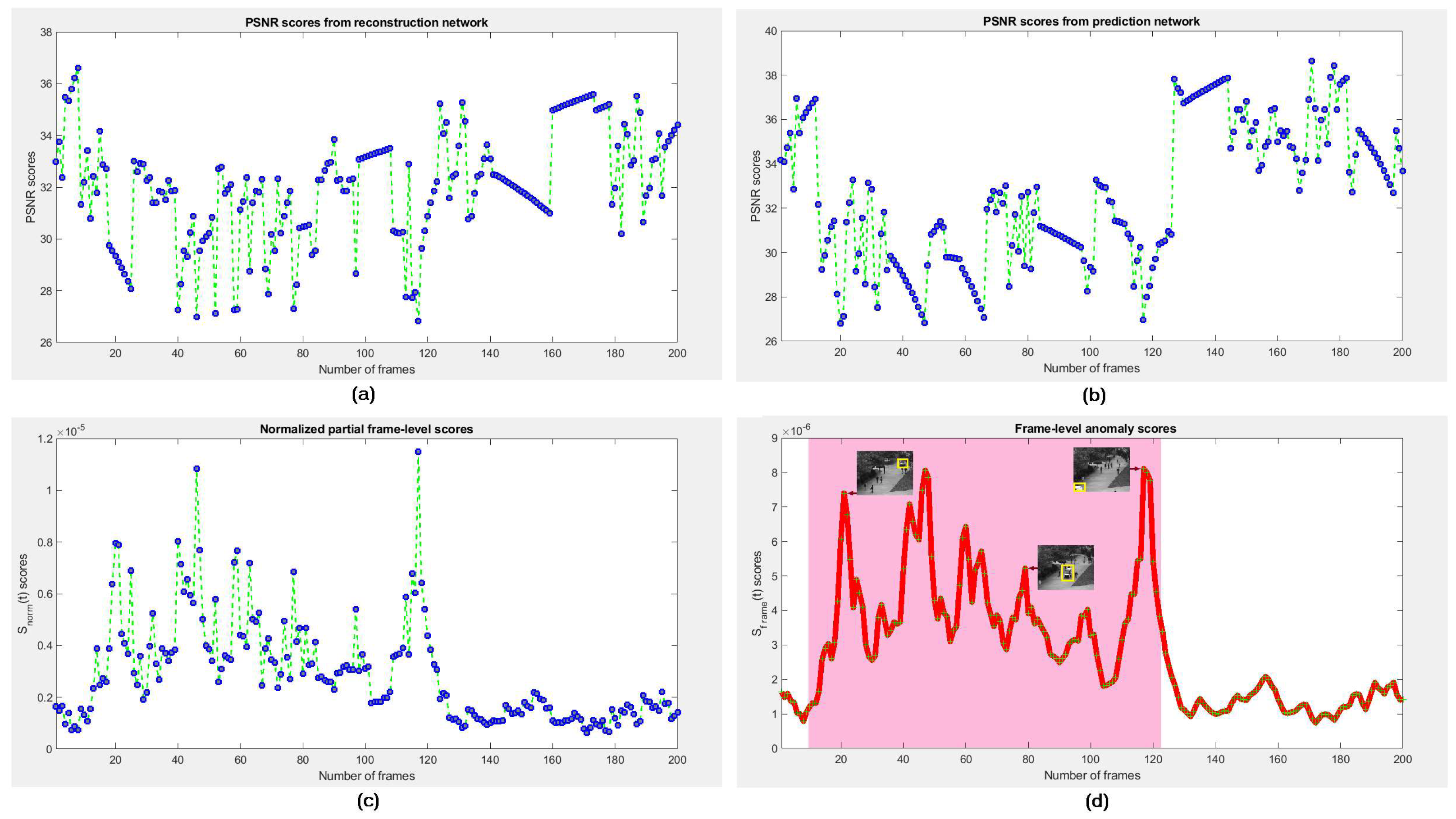
We assume that if any frame $f_t$ holds an appearance anomaly (e.g., someone carrying a gun) then the rNet can improve its determinability, whereas if $f_t$ contains a motion anomaly (e.g., people fighting on the street) the pNet can improve its determinability. Therefore, we bring the error scores of appearance and prediction into a cascaded score to compute the final error score of each frame for detecting its anomalousness. We evaluate the anomaly of appearance based on reconstruction error of the entire frame. This technique preserves the complete appearance of target objects in frame. We define pixel-wise partial anomaly score individually estimated on the prediction error of $PSN{R}_p$ and the reconstruction error of $PSN{R}_r$ from prediction and reconstruction networks, respectively, sharing for the same frame as:

$$\begin{array}{cc}\hfill PSN{R}_r& =20lo{g}_{10}\left(\frac{255}{\sqrt{\frac{1}{WH}{\sum }_{x=1}^W{\sum }_{y=1}^H{\left({f_t}_{x,y}-{\widehat{f_t^{\prime }}}_{x,y}\right)}^2}}\right)\hfill \end{array}$$

(13)

$$\begin{array}{cc}\hfill PSN{R}_p& =20lo{g}_{10}\left(\frac{255}{\sqrt{\frac{1}{WH}{\sum }_{x=1}^W{\sum }_{y=1}^H{\left({f_t}_{x,y}-{\widehat{f_t}}_{x,y}\right)}^2}}\right),\hfill \end{array}$$

(14)

where W, H, $(x,y)$ are the width, height, and spatial index of the frame, respectively. The maximum pixel value of an image is 255. Large $PSN{R}_r$ or $PSN{R}_p$ of a frame hints that it is more likely to be normal. Roughly, it is possible to use $PSN{R}_r$ or $PSN{R}_p$ for determining whether an abnormal event has occurred. For example, if $PSN{R}_r$ or $PSN{R}_p$ is greater than any defined threshold, the frame is normal, otherwise abnormal. Nevertheless, it expects more refinement for better performance.

The partial frame-level score of the t-th frame $S_{part}\left(t\right)$ is computed as a weighted combination of the two incomplete scores as follows:

$$\begin{array}{cc}\hfill S_{part}\left(t\right)& =\left({\sigma }_1\right)\left({\omega }_1\right)\left(PSN{R}_r\right)+\left({\sigma }_2\right)\left({\omega }_2\right)\left(PSN{R}_p\right),\hfill \end{array}$$

(15)

where ${\omega }_1$ and ${\omega }_2$ are the weights, which normalize the two scores to the same scale. They can be calculated on the training data of n images using Equations (16) and (17) as:

$$\begin{array}{cc}\hfill {\omega }_1& =\frac{1}{10}lo{g}_{10}\left(\frac{1}{n}\sum _{i=1}^{n}PSN{R}_{r_i}\right)\hfill \end{array}$$

(16)

$$\begin{array}{cc}\hfill {\omega }_2& =\frac{1}{10}lo{g}_{10}\left(\frac{1}{n}\sum _{i=1}^{n}PSN{R}_{p_i}\right).\hfill \end{array}$$

(17)

The hyper parameters of ${\sigma }_1>0$ and ${\sigma }_2>0$ are used to control the contribution of corresponding score to the summation, which can be adjusted appropriately for the importance of the appearance and motion. We perform a normalization of $S_{part}\left(t\right)$ using Equation (18) as:

$$S_{norm}\left(t\right)=e^{-{\left(\frac{S_{part}\left(t\right)}{\lambda }\right)}^{\nu }},$$

(18)

where $\nu >0$ and $\lambda >0$ belong to shape and scale parameters, respectively [74]. The occurrence of abnormal events in video has continuity, i.e., abnormal events cannot appear in a single frame, but appear in multiple consecutive frames. Consequently, we utilize not only the current frame but also the past and future frames to compute the final anomaly score using Equation (19) as:

$$S_{frame}\left(t\right)=\frac{1}{{\eta }^2}\sum _{i=0}^{\eta }(\eta -i)\left(S_{norm}(t\pm i)\right),$$

(19)

where the anomaly score of the t-th frame $S_{frame}\left(t\right)$ consists of the $S_{norm}\left(t\right)$ as current frame and the $S_{norm}(t\pm i)$ with $i=1,2,\dots ,\eta$ of $\eta$ past and future frames. The score of $S_{frame}\left(t\right)$ estimated from a frame of abnormal event is expected to be higher compared with the ones of normal event. Therefore, we can predict whether a frame is normal or abnormal based on $S_{frame}\left(t\right)$. One can set a threshold to distinguish normal or abnormal frames.

8. Larger Error Gap Guaranteed by rpNet

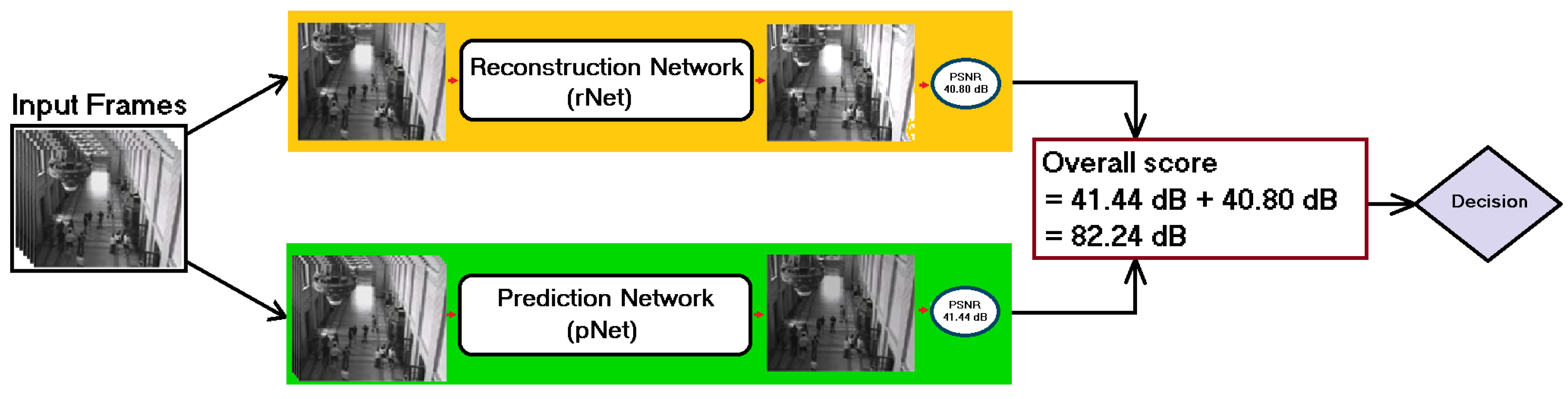
Ideally, both pNet and rNet can produce their own outputs. We assume that the output of either pNet or rNet can individually provide necessary anomaly scores, but may not provide sufficient anomaly scores used for anomaly detection. The gain of the rpNet individually relies on pNet and rNet. The overall gain of the rpNet equals to the product of the individual gain of pNet and rNet. Mathematically, if $G_1$ and $G_2$ indicate the gains of pNet and rNet, respectively, then the overall gain $G_{overall}$ can be formulated by Equation (20) as:

$$G_{overall}=\left(G_1\right)\left(G_2\right).$$

(20)

When the gain of pNet and rNet applies the decibel (dB) expression, the Equation (20) yields:

$$\begin{array}{}\mathrm{(21)}& log\left(G_{overall}\right)=log\left(\left(G_1\right)\left(G_2\right)\right)\hfill \mathrm{(22)}& \hspace{1em}\hspace{0.17em}\hspace{1em}\hspace{1em}\hspace{1em}\hspace{1em}=log\left(G_1\right)+log\left(G_2\right)\hfill \end{array}$$

$$\begin{array}{cc}\hfill G_{overall}\mathrm{dB}& =G_1\mathrm{dB}+G_2\mathrm{dB}.\hfill \end{array}$$

(23)

For example, Figure 10 conveys a simplified schematic diagram of the rpNet along with any instance of video frames if pNet and rNet achieve 41.44 dB and 40.80 dB, respectively, then the overall process has a gain of 82.24 dB.

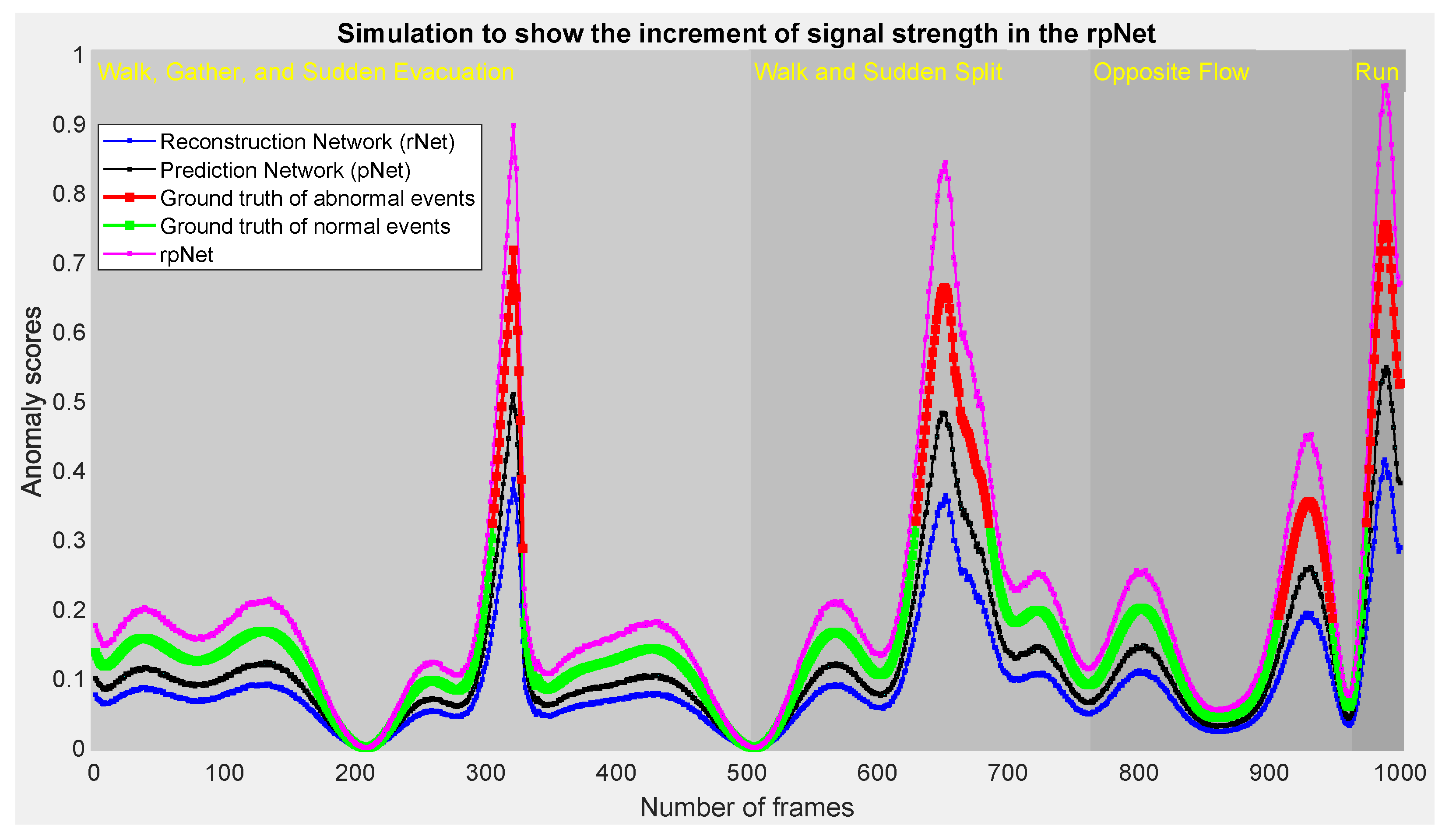
Using a simple simulation, we wish to explain that the rpNet can provide better anomalous detection results by providing higher anomaly scores for abnormal cases in videos than that of either pNet or rNet individually. Explicitly, the rpNet can provide an improved reconstruction error gap by increasing the output signal strength of pNet and rNet.

Assume that a hypothetical video surveillance system has captured the following four scenarios of people: (i) Normal walk and gather but sudden evacuation after an unwanted event, (ii) normal walk and sudden split after an incident, (iii) someone intentionally passing opposite of the main stream, and (iv) sudden run after an explosion. In addition, assume that both pNet and rNet are trained with a normal video cases and can detect those abnormal video events by providing the anomaly scores as depicted in Figure 11. The ground truths for four scenarios are given, but the anomaly scores of the rpNet are calculated.

Table 2. Qualitative and quantitative analysis of the simulated normal and abnormal video events in Figure 11.

Measures	Walk, Gather, Evacuate			Walk, Sudden Split			Opposite Flow			Sudden Run
	rNet	pNet	rpNet	rNet	pNet	rpNet	rNet	pNet	rpNet	rNet	pNet	rpNet
Ground truth frame start ($g_s$)	305	305	305	629	629	629	907	907	907	974	974	974
Ground truth frame end ($g_e$)	328	328	328	685	685	685	948	948	948	1000	1000	1000
First detected abnormal frame ($f_d$)	317	311	302	645	636	625	928	915	903	982	978	975
Last detected abnormal frame ($l_d$)	325	326	328	657	669	690	928	943	950	988	991	1000
Number of false positive frames ($f_p$)	0	0	3	0	0	4	0	0	4	0	0	1
Number of true positive frames ($t_p$)	8	15	26	12	33	65	1	28	47	6	13	25
Number of false negative frames ($f_n$)	15	8	3	44	23	9	41	13	6	20	13	1
Number of true negative frames ($t_n$)	477	477	468	204	204	182	158	159	143	14	14	13
Sum ($T_f=t_p+t_n+f_p+f_n$)	500	500	500	260	260	260	200	200	200	40	40	40
Recall Rate ($t_p/(t_p+f_n)$)	0.348	0.652	0.896	0.214	0.589	0.878	0.024	0.683	0.887	0.231	0.500	0.961
Specificity ($t_n/(t_n+f_p)$)	1	1	0.994	1	1	0.978	1	1	0.973	1	1	0.929
False positive rate = (1 − Specificity)	0	0	0.006	0	0	0.021	0	0	0.027	0	0	0.071
Precision rate ($t_p/(t_p+f_p)$)	1	1	0.897	1	1	0.942	1	1	0.922	1	1	0.961
Accuracy ($ACC=(t_p+t_n)/T_f$)	0.970	0.984	0.988	0.831	0.911	0.950	0.795	0.935	0.950	0.500	0.675	0.950
RMSE at rising edge (${\Gamma }_r$) for rNet	$\sqrt{\frac{905}{4}}\approx 15.0416$ using ${\Gamma }_r=\sqrt{\frac{1}{4}{\sum }_{i=1}^4{(g_s\left(i\right)-f_d\left(i\right))}^2}$
CV(${\Gamma }_r$) at rising edge for rNet	$\frac{15.0416}{2815}\approx 0.0053$ using $CV\left({\Gamma }_r\right)=\frac{{\Gamma }_r}{\frac{1}{4}{\sum }_{i=1}^4{g}_s}$
RMSE at falling edge (${\Gamma }_f$) for rNet	$\sqrt{\frac{1337}{4}}\approx 18.2825$ using ${\Gamma }_f=\sqrt{\frac{1}{4}{\sum }_{i=1}^4{(g_e\left(i\right)-l_d\left(i\right))}^2}$
CV(${\Gamma }_f$) at falling edge for rNet	$\frac{18.2825}{2961}\approx 0.0062$ using $CV\left({\Gamma }_f\right)=\frac{{\Gamma }_f}{\frac{1}{4}{\sum }_{i=1}^i{g}_e}$
${\Gamma }_r$ and CV(${\Gamma }_r$) for pNet	$\sqrt{\frac{165}{4}}\approx 6.4226$ and $\frac{6.4226}{2815}\approx 0.0023$
${\Gamma }_f$ and CV(${\Gamma }_f$) for pNet	$\sqrt{\frac{366}{4}}\approx 9.5656$ and $\frac{9.5656}{2961}\approx 0.0032$
${\Gamma }_r$, CV(${\Gamma }_r$), ${\Gamma }_f$, CV(${\Gamma }_f$) for rpNet	$\sqrt{\frac{42}{4}}\approx 3.2404$, $\frac{3.2404}{2815}\approx 0.0012$, $\sqrt{\frac{29}{4}}\approx 2.6926$, $\frac{2.6926}{2961}\approx 0.0009$
ROC curve analysis	$\mathbf{AUC}\approx \mathbf{0}.\mathbf{6739}$ for rNet, $\mathbf{AUC}\approx \mathbf{0}.\mathbf{8415}$ for pNet, $\mathbf{AUC}\approx \mathbf{0}.\mathbf{9731}$ for rpNet
Mean ACC gain obtained by rpNet	rpNet was $\frac{0.9595}{0.7740}-1=\mathbf{23}.\mathbf{97}\%$, $\frac{0.9595}{0.8762}-1=\mathbf{9}.\mathbf{51}\%$,
	and $\mathbf{16}.\mathbf{74}\%$ more accurate over rNet, pNet, and their mean ACC, respectively.
AUC gain obtained by rpNet	rpNet performed $\frac{0.9731}{0.6739}-1=\mathbf{44}.\mathbf{40}\%$, $\frac{0.9731}{0.8415}-1=\mathbf{15}.\mathbf{64}\%$,
	and $\mathbf{30}.\mathbf{02}\%$ better than rNet, pNet, and their mean AUC, respectively.

shows the analyzing report of Figure 11 in qualitatively and quantitatively. The mean ACC scores of pNet and rNet are 0.7740 and 0.8762, respectively. The mean ACC of the rpNet is 0.9595, which is definitely higher than those scores. To gain such ACC score, the rpNet has to come up against a mean false alarm rate of 0.0313. Nevertheless, on the average, the rpNet achieves 16.74% better ACC score than the mean ACC score of the pNet and rNet. At the rising edge, the values of root MSE (RMSE) are 15.0416, 6.4226, and 3.2404 for the rNet, pNet, and rpNet, respectively. The RMSE is $10.7321/3.2404=3.312$ times less in the rpNet compared with the mean RMSE of rNet and pNet. Similarly, at the falling edge, the RMSE is $13.9240/2.6926=5.1712$ times less in the rpNet. The coefficient of variation of the RMSE, denoted as CV(RMSE), is $0.0038/0.0012=3.1667$ and $0.0047/0.0009=5.2222$ times less in the rpNet at rising and falling edges, respectively, compared with the mean CV(RMSE) of rNet and pNet.

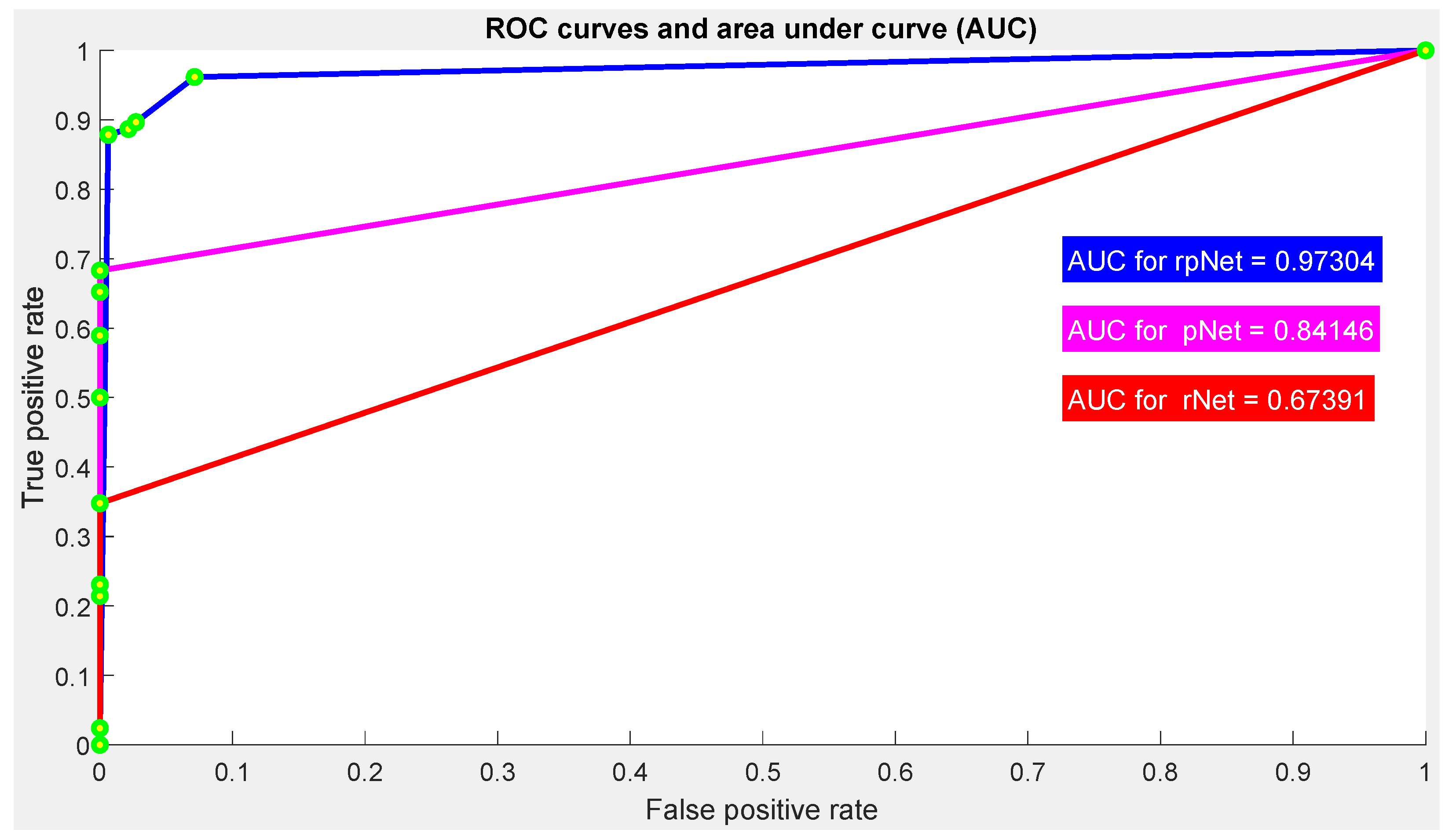
Taking into account the data in Table 2, upon ROC curve analysis the scores of 0.674, 0.841, and 0.973 can be obtained from rNet, pNet, and rpNet, respectively. From Figure 12, it is noticeable that the rpNet became the highest performative model considering data in Table 2. The rpNet achieves 1.3002 times or 30.02% better AUC scores than the mean AUC score of rNet and pNet. Explicitly, the simulated events in Figure 11 show evidence that the rpNet can guarantee larger error gap on the identical ground of both rNet and pNet. This proposition is also supported by the practical results from the experimental setup.

In essence, the aforementioned straightforward simulation shows that the rpNet is capable of achieving certain incremental factor of the reconstruction error gap by increasing the signal strength of the anomaly scores.

9. Experimental Setup and Results

Our implementation was performed by Python based on the TensorFlow framework [75]. Both training and evaluation of the model were performed on an Intel ${}^{\circledR }$ Core ${}^{TM}$ i7-7800X CPU @3.50 GHz along with NVIDIA’s graphics card GeForce GTX 1080. We used the Adam optimizer [64] for training and set the learning rate to 0.0001 and 0.00001 for the generator and discriminator, respectively. The input images are resized to $256\times 256$ pixels and converted to gray-scale. We trained our model using five publicly available datasets, as illustrated in

Table 3. Comparison of various specifications of crowd datasets and their available web links. $H\Rightarrow$ height, $W\Rightarrow$ width.

Dataset	Source	Counting			Videos				Annotation			Number of Frames			Anomaly Events	Dataset Link
		Scene	Duration	Anomaly	Training	Testing	Total	$\mathit{H}\times \mathit{W}$ of Frame	Using	Level	Count	Training	Testing	Total
UCSD-Ped1 [31] (2008)	Using 1st outdoor surveillance camera.	5	5 min	40	34	36	70	$158\times$238	Human	Pixel	NA	6800	7200	14,000	Circulation of non-pedestrian entities in the walkways and anomalous pedestrian motion patterns.	http://www.svcl.ucsd.edu/projects/anomaly/dataset.htm, (accessed on 2 January 2023)
UCSD-Ped2 [31] (2008)	Using 2nd outdoor surveillance camera.	5	5 min	12	16	12	28	$240\times$360	Human	Pixel	NA	2550	2010	4560	Circulation of non-pedestrian entities in the walkways and anomalous pedestrian motion patterns.	http://www.svcl.ucsd.edu/projects/anomaly/dataset.htm, (accessed on 2 January 2023)
UMN [36] (2009)	Synthetic dataset [76,77].	3	4.3 min	11	Unavailable	Unavailable	11	$480\times 640$$240\times$320	Software	Temporal	Unavailable	Unavailable	Unavailable	7725	In each video crowd walks randomly. Everyone starts running suddenly, which is marked as an anomaly.	http://mha.cs.umn.edu/proj_events.shtml#crowd, (accessed on 2 January 2023)
CUHK-Avenue [32] (2013)	Captured in CUHK campus avenue.	5	30 min	47	16	21	37	$360\times$640	Human	Pixel Frame	NA	15,328	15,324	30,652	Strange actions, wrong directions, unexpected objects. The ground truth of anomalous objects is marked by a rectangle.	www.cse.cuhk.edu.hk/leojia/projects/detectabnormal/dataset.html, (accessed on 2 January 2023)
Shanghai Tech Campus [18] (2017)	University campus, surveillance cameras.	13	NA	130	238	199	437	$2048\times$2048	Human	Pixel	NA	274515	42,883	317,398	Anomalies caused by sudden motion, including chasing and brawling.	https://svip-lab.github.io/dataset/campus_dataset.html, (accessed on 2 January 2023)

, namely UCSD-Ped1 [31], UCSD-Ped2 [31], CUHK-Avenue [32], ShanghaiTech-Campus [18], and UMN [36] datasets with normal events. For evaluation, we used both normal and abnormal frames of those datasets. The training procedure was iterated up to a maximum of 100 epochs. The batch size was set to 4. AUC metric was used to evaluate the overall model performance.

As our methodology possesses six combinational models, namely AE-Unet (Ours), AEcUnet (Ours), AEnUnet (Ours), AEcnUnet (Ours), AEaUnet (Ours), and AEcaUnet (Ours), we conduct experiment each of them individually.

Table 4. List of parameters and their used values.

Dataset	Value of Parameters															Ratio of
	${\mathit{\lambda }}_{{\mathbf{int}}_{\mathit{p}}}$	${\mathit{\lambda }}_{{\mathbf{gd}}_{\mathit{p}}}$	${\mathit{\lambda }}_{{\mathbf{int}}_{\mathit{r}}}$	${\mathit{\lambda }}_{{\mathbf{gd}}_{\mathit{r}}}$	${\mathit{\lambda }}_{\mathbf{mot}}$	${\mathit{\lambda }}_{\mathbf{adg}}$	Mean $\mathbf{\Gamma }$	$\mathit{d}\mathit{e}\mathit{A}\mathit{t}\mathit{t}$	${\mathit{\omega }}_1$	${\mathit{\omega }}_2$	${\mathit{\sigma }}_1$	${\mathit{\sigma }}_2$	$\mathit{\nu }$	$\mathit{\lambda }$	$\mathit{\eta }$	Training	Testing
Ped1 [31]	1.05	1.03	1.05	1.05	1.90	0.05	0.357	50	0.931	0.869	1	1	0.515	1.615	2	49%	51%
Ped2 [31]	1.05	1.10	1.06	1.05	1.85	0.05	0.195	60	0.926	0.851	1	1	0.715	1.515	2	56%	44%
Avenue [32]	1.09	1.19	1.02	1.12	2.13	0.05	0.114	45	0.902	0.813	1	1	0.505	1.365	2	50%	50%
Campus [18]	1.07	1.04	1.05	1.05	2.19	0.05	0.428	55	0.942	0.877	1	1	0.355	1.125	2	85%	15%
UMN [36]	1.02	1.05	1.08	1.10	2.07	0.05	0.126	75	0.945	0.863	1	1	0.605	1.450	3	60%	40%

lists miscellaneous parameter values used during experiments. Figure 13, Figure 14, Figure 15, Figure 16 and Figure 17 demonstrate sample results of AEcaUnet (Ours) using parameters in Table 4. For a better visualization, the rectangles on camera view images were highlighted manually. The pink region indicates the ground truth of abnormal events. It is observable that the partial results of prediction network are superior to that of reconstruction network. This is due to the fact that the prediction network is capable of being extracted for better quality of features from the available videos. However, the partial results of both networks contribute as a complement towards the final performance of each model by confirming certain degree of augmentation of the reconstruction error gap.

10. Experimental Result Comparison

In the literature, there are widely used common datasets that are used to test the performance of different deep models, while other datasets were mainly used to test the generalization ability of those models for detecting crowd anomaly in video streams.

Table 5. Frame-level AUC score comparison of miscellaneous methods and datasets. Column-wise the best numerical result is shown in bold.

Year	Models	Various Popular Crowd Datasets
		Ped1 [31]	Ped2 [31]	Avenue [32]	Campus [18]	UMN [36]
Before 2020	Liu et al. [2]	0.831	0.954	0.849	0.728	-
	Hasan  et al. [1]	0.750	0.850	0.800	0.609	-
	LuoLG [78]	0.755	0.881	0.770	-	-
	Luo  et al. [18]	-	0.922	0.817	0.680	-
	Nguyen  et al. [27]	-	0.962	0.869	-	-
	Ionescu et al. [22]	0.684	0.822	0.806	-	-
2020	WangCYJT [79]	0.834	0.963	0.883	0.766	-
	Chen et al. [80]	0.872	0.965	0.873	-	-
	Dong et al. [81]	-	0.956	0.849	0.737	-
	Fan et al. [82]	0.949	0.922	0.834	-	-
	Nawaratne et al. [83]	0.752	0.911	0.768	-	-
	Wang et al. [84]	0.867	0.991	0.899	-	-
	WuLLSS [85]	0.824	0.928	0.855	-	-
	Yang et al. [86]	0.935	0.937	0.832	-	-
	Zahid et al. [87]	0.585	0.789	0.750	0.940	-
	Zhou et al. [88]	0.839	0.960	0.860	-	-
	Doshi et al. [89]	-	0.978	0.864	0.716	-
	Pang et al. [90]	0.720	0.830	-	-	0.993
	Roy et al. [91]	0.850	0.975	0.870	0.810	0.997
	Wu et al. [92]	0.840	0.924	-	-	0.993
	Ji et al. [93]	0.840	0.980	0.780	-	-
	Lu et al. [94]	0.863	0.962	0.858	0.779	-
	Ramachandra et al. [95]	0.860	0.940	0.872	-	-
	Tang et al. [96]	0.830	0.960	0.840	0.72	-
	Almazroey et al. [97]	0.937	0.833	0.875	-	-
	Wu0S [98]	0.830	0.960	0.870	-	0.890
	Lee et al. [99]	-	0.966	0.900	0.762	0.996
	Prawiro et al. [100]	0.840	0.960	0.860	-	-
	Song et al. [101]	0.905	0.907	0.892	0.700	-
	Yan et al. [102]	0.750	0.910	0.796	-	-
2021	Sun et al. [103]	0.902	0.910	0.889	0.922	-
	Xia et al. [104]	0.880	0.966	0.922	-	0.970
	Feng et al. [105]	-	0.970	0.860	0.777	-
	Zhang et al. [106]	-	0.954	0.868	0.736	-
	Wu et al. [107]	0.885	0.988	0.847	0.728	-
	Vu et al. [108]	0.850	0.960	0.920	0.937	-
	Mu et al. [109]	0.952	0.947	0.897	0.921	-
	LiLS [110]	0.853	0.955	0.891	0.740	-
	LiCL [111]	0.905	0.929	0.835	-	0.980
	Cai et al. [112]	-	0.968	0.873	0.742	-
	Saypadith et al. [113]	0.853	0.957	0.868	0.730	-
	Doshi et al. [26]	-	0.972	0.864	0.709	-
	Luo et al. [114]	-	0.922	0.835	0.696	-
	Gutoski et al. [115]	0.719	0.893	0.847	-	0.992
2022	Zhong et al. [3]	0.826	0.977	0.889	0.707	-
	Chang  et al. [116]	-	0.967	0.871	0.737	-
	Esquivel et al. [117]	0.710	0.870	0.830	0.870	-
	Park et al. [118]	-	0.960	0.850	0.720	-
	Doshi et al. [119]	-	0.970	0.887	0.736	-
	Li et al. [120]	0.812	0.971	0.866	0.782	-
	Hao et al. [121]	0.825	0.969	0.866	0.738	-
	Zhang et al. [13]	0.836	0.959	0.852	0.727	-
	Alafif et al. [122]	0.828	0.957	-	-	0.981
	Shao et al. [123]	0.776	0.949	0.853	0.717	-
	Zou et al. [124]	-	0.973	0.872	0.727	-
	Zhou et al. [125]	-	0.974	0.926	0.749	-
	Hu et al. [126]	0.807	0.853	0.810	-	-
	Zhang et al. [127]	0.942	0.929	0.805	0.803	0.988
	Wang et al. [128]	0.880	0.890	0.870	-	-
	Liu et al. [129]	-	0.981	0.898	0.738	-
	Feng et al. [130]	0.836	0.908	0.813	-	-
	Cho et al. [131]	-	0.992	0.880	0.763	-
	ParkLCL [132]	-	0.958	0.854	0.724	-
	Le et al. [133]	-	0.974	0.867	0.736	-
	Liu et al. [28]	0.851	0.966	0.865	-	-
2023	AE-Unet (Ours)	0.848	0.902	0.825	0.734	0.930
	AEcUnet (Ours)	0.862	0.934	0.863	0.761	0.965
	AEnUnet (Ours)	0.872	0.957	0.871	0.774	0.977
	AEcnUnet (Ours)	0.888	0.971	0.874	0.782	0.976
	AEaUnet (Ours)	0.875	0.969	0.887	0.780	0.980
	AEcaUnet (Ours)	0.918	0.989	0.916	0.798	0.987

compares frame-level AUC scores among miscellaneous methods and the most frequently used crowd datasets.

From Table 5, it is notable that our method could not demonstrate an outright accuracy score. However, from Table 5, it is hard to notice the best performative method as an individual method could not achieve an absolute better performance. For example, Mu et al. [109], Cho et al. [131], Xia et al. [104], Zahid et al. [87], and Roy et al. [91] achieved the best AUC scores of 0.952, 0.992, 0.922, 0.940, and 0.997 from UCSD-Ped1 [31], UCSD-Ped2 [31], CUHK-Avenue [32], ShanghaiTech-Campus [18], and UMN [36], respectively. Unambiguously, considering experimental results in Table 5, it is very hard to find that one algorithm is better than its alternatives. Usually, the nonparametric statistical analysis can be used for superiority measure [134], but all models were not tested against always the same five datasets in Table 5. Henceforth, based on the chosen datasets by the authors of various models in Table 5, mainly for statistical analysis, we can divide the tabular data in Table 5 into six following groups:

${\mathbf{G}}_{\mathbf{1}}$

Methods of this group were tested against the datasets of UCSD-Ped1 [31], UCSD-Ped2 [31], CUHK-Avenue [32], ShanghaiTech-Campus [18], and UMN [36] or the methods existed before 2020 (i.e., Table 6).

${\mathbf{G}}_{\mathbf{2}}$

Methods of this group were tested against the datasets of UCSD-Ped2 [31], CUHK-Avenue [32], and ShanghaiTech-Campus [18] (i.e., Table 7).

${\mathbf{G}}_{\mathbf{3}}$

Methods of this group were tested against the datasets of UCSD-Ped1 [31], UCSD-Ped2 [31], and CUHK-Avenue [32] (i.e., Table 8).

${\mathbf{G}}_{\mathbf{4}}$

Methods of this group were tested against the datasets of UCSD-Ped1 [31], UCSD-Ped2 [31], CUHK-Avenue [32], and ShanghaiTech-Campus [18] (i.e., Table 9).

${\mathbf{G}}_{\mathbf{5}}$

Methods of this group were tested against the datasets of UCSD-Ped1 [31], UCSD-Ped2 [31], CUHK-Avenue [32], and UMN [36] (i.e., Table 10).

${\mathbf{G}}_{\mathbf{6}}$

Methods of this group were tested against the datasets of UCSD-Ped1 [31], UCSD-Ped2 [31], and UMN [36] (i.e., Table 11).

The frame-level failure score of AUC (fAUC) is defined by Equation (24) as:

$$fAUC=1-AUC.$$

(24)

Table 6. The fAUC scores of ${\mathbf{G}}_{\mathbf{1}}$. Column-wise the best numerical result is shown in bold.

Models	Obtained fAUC Scores from Different Datasets					Mean of fAUC Scores
	Ped1 [31]	Ped2 [31]	Avenue [32]	Campus [18]	UMN [36]	Arithmetic	Geometric	Harmonic
Zhang et al. [127]	0.0580	0.0710	0.1950	0.1970	0.0120	0.1066	0.0717	0.0400
Roy et al. [91]	0.1500	0.0250	0.1300	0.1900	0.0030	0.0996	0.0488	0.0127
Liu et al. [2]	0.1690	0.0460	0.1510	0.2720	-	0.1595	0.1337	0.1054
Hasan  et al. [1]	0.2500	0.1500	0.2000	0.3910	-	0.2478	0.2327	0.2195
LuoLG [78]	0.2450	0.1190	0.2300	-	-	0.1980	0.1886	0.1782
Luo  et al. [18]	-	0.0780	0.1830	0.3200	-	0.1937	0.1659	0.1401
Nguyen  et al. [27]	-	0.0380	0.1310	-	-	0.0845	0.0706	0.0589
Ionescu et al. [22]	0.3160	0.1780	0.1940	-	-	0.2293	0.2218	0.2153
AE-Unet (Ours)	0.1520	0.0980	0.1750	0.2660	0.0700	0.1522	0.1372	0.1233
AEcUnet (Ours)	0.1380	0.0660	0.1370	0.2390	0.0350	0.1230	0.1009	0.0801
AEnUnet (Ours)	0.1280	0.0430	0.1290	0.2260	0.0230	0.1098	0.0819	0.0577
AEcnUnet (Ours)	0.1120	0.0290	0.1260	0.2180	0.0240	0.1018	0.0735	0.0512
AEaUnet (Ours)	0.1250	0.0310	0.1130	0.2200	0.0200	0.1018	0.0719	0.0482
AEcaUnet (Ours)	0.0820	0.0110	0.0840	0.2020	0.0130	0.0784	0.0457	0.0254

Table 6. The fAUC scores of ${\mathbf{G}}_{\mathbf{1}}$. Column-wise the best numerical result is shown in bold.

Models	Obtained fAUC Scores from Different Datasets					Mean of fAUC Scores
	Ped1 [31]	Ped2 [31]	Avenue [32]	Campus [18]	UMN [36]	Arithmetic	Geometric	Harmonic
Zhang et al. [127]	0.0580	0.0710	0.1950	0.1970	0.0120	0.1066	0.0717	0.0400
Roy et al. [91]	0.1500	0.0250	0.1300	0.1900	0.0030	0.0996	0.0488	0.0127
Liu et al. [2]	0.1690	0.0460	0.1510	0.2720	-	0.1595	0.1337	0.1054
Hasan  et al. [1]	0.2500	0.1500	0.2000	0.3910	-	0.2478	0.2327	0.2195
LuoLG [78]	0.2450	0.1190	0.2300	-	-	0.1980	0.1886	0.1782
Luo  et al. [18]	-	0.0780	0.1830	0.3200	-	0.1937	0.1659	0.1401
Nguyen  et al. [27]	-	0.0380	0.1310	-	-	0.0845	0.0706	0.0589
Ionescu et al. [22]	0.3160	0.1780	0.1940	-	-	0.2293	0.2218	0.2153
AE-Unet (Ours)	0.1520	0.0980	0.1750	0.2660	0.0700	0.1522	0.1372	0.1233
AEcUnet (Ours)	0.1380	0.0660	0.1370	0.2390	0.0350	0.1230	0.1009	0.0801
AEnUnet (Ours)	0.1280	0.0430	0.1290	0.2260	0.0230	0.1098	0.0819	0.0577
AEcnUnet (Ours)	0.1120	0.0290	0.1260	0.2180	0.0240	0.1018	0.0735	0.0512
AEaUnet (Ours)	0.1250	0.0310	0.1130	0.2200	0.0200	0.1018	0.0719	0.0482
AEcaUnet (Ours)	0.0820	0.0110	0.0840	0.2020	0.0130	0.0784	0.0457	0.0254

Table 6 presents the fAUC scores of ${\mathbf{G}}_{\mathbf{1}}$ group with related evaluation. Although many methods are related to this group, rigorous statistical analysis is very difficult to perform. For example, the method of Nguyen et al. [27] was only tested on two datasets, whereas the method of Zhang et al. [127] was tested on five datasets. Thus, instead of using rigorous statistical analysis, for evaluation we use arithmetic, geometric, and harmonic means only. The method of Zhang et al. [127] presented the best performance from UCSD-Ped1 [31], whereas AEcaUnet (Ours) demonstrated the best performance from UCSD-Ped2 [31] and CUHK-Avenue [32]. The method of Roy et al. [91] showed slightly better performance from UMN [36]. However, methods of Zhang et al. [127], Roy et al. [91], and AEcaUnet (Ours) showed approximately the same performance from ShanghaiTech-Campus [18]. Nevertheless, the overall performance of AEcaUnet (Ours) is better than that of either Roy et al. [91] or Zhang et al. [127]. Explicitly, by referring to Table 6, AEcaUnet (Ours) seemingly showed the best performance from ${\mathbf{G}}_{\mathbf{1}}$.

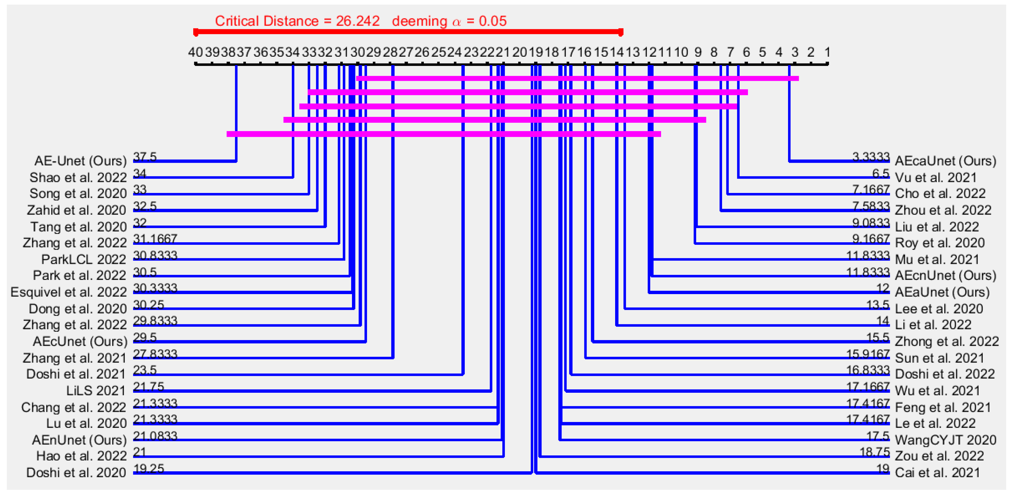
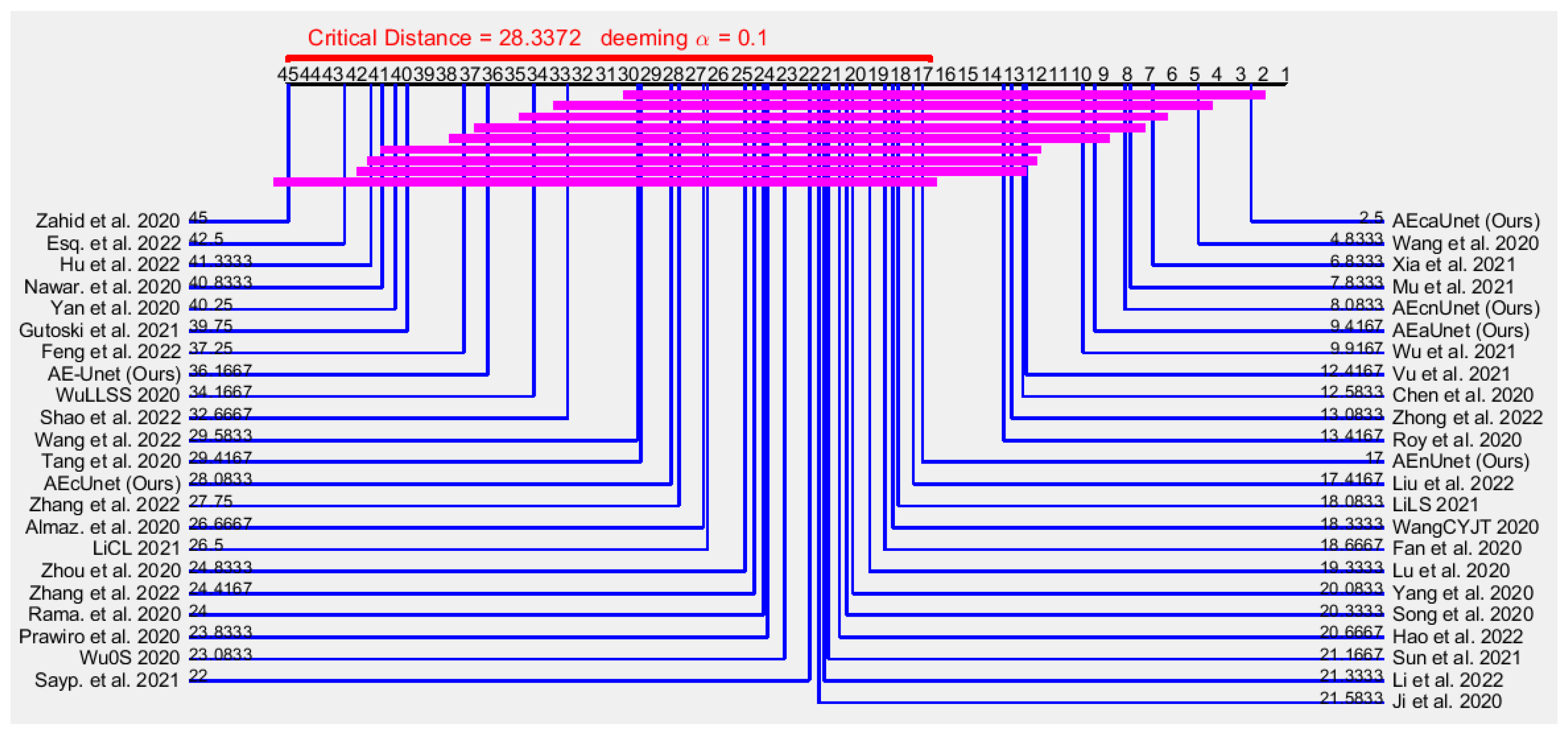
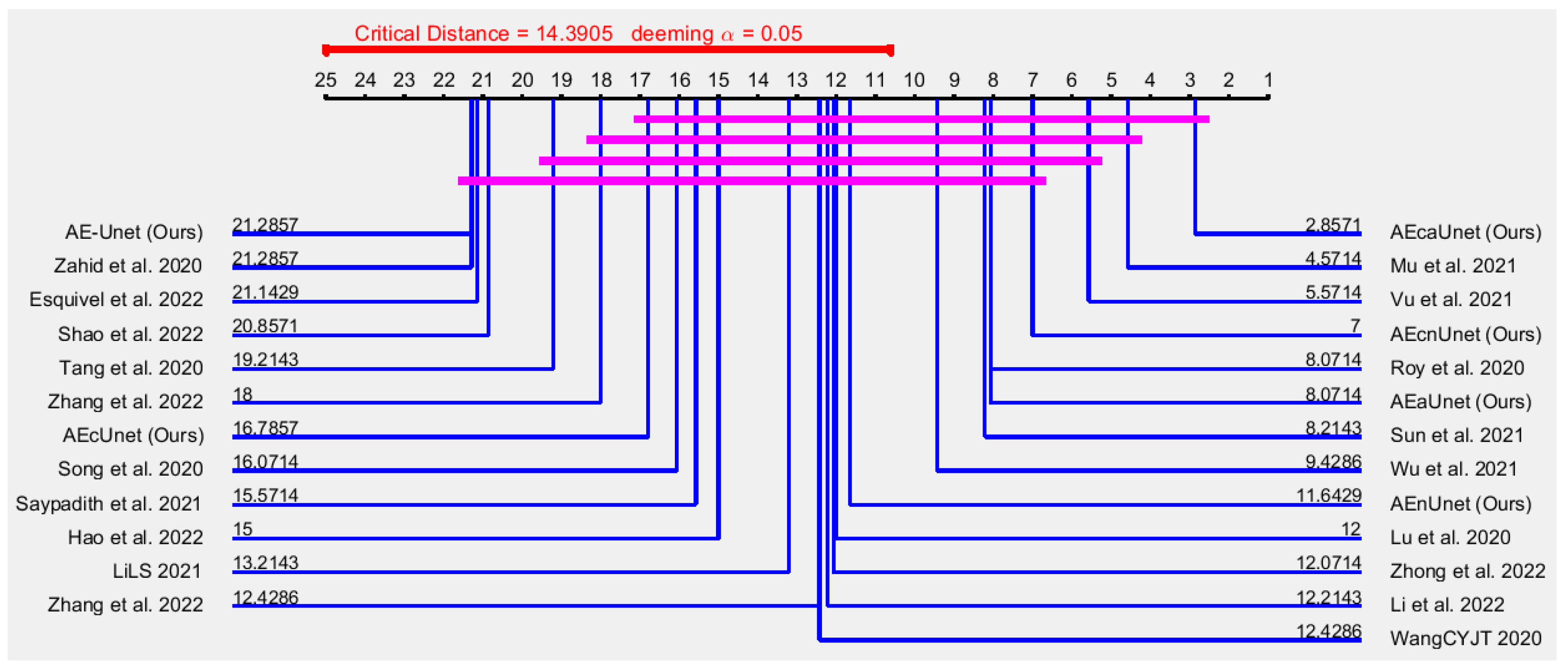
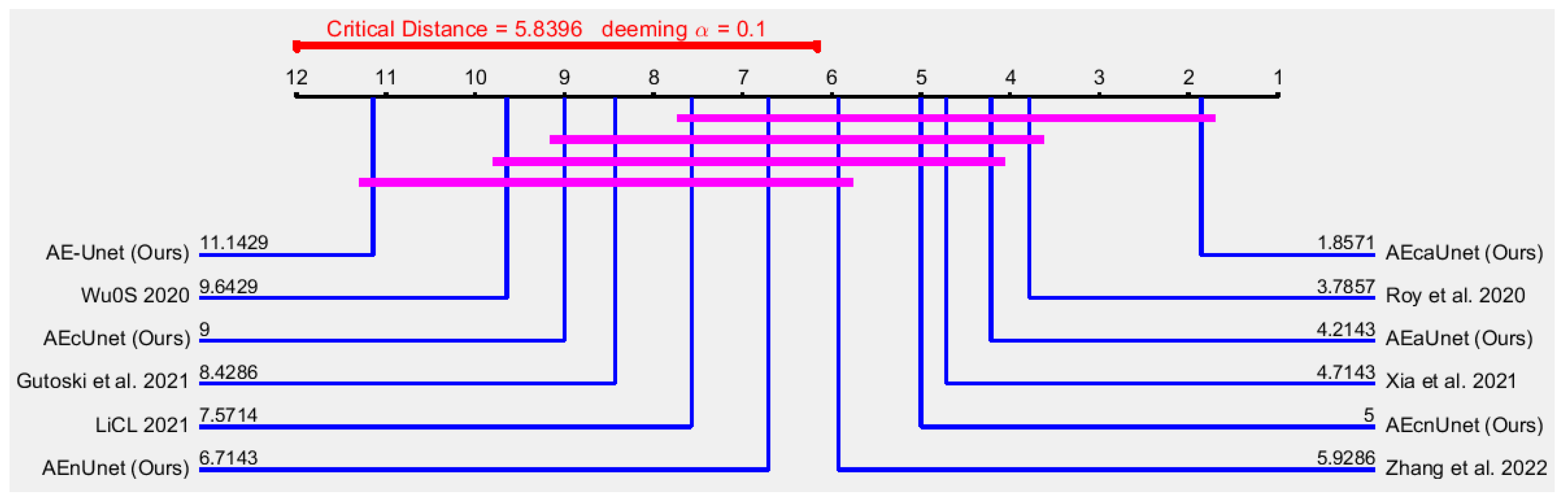
For ${\mathbf{G}}_{\mathbf{2}}$, ${\mathbf{G}}_{\mathbf{3}}$, ${\mathbf{G}}_{\mathbf{4}}$, and ${\mathbf{G}}_{\mathbf{5}}$, on the other hand, it is not show any direct indication of superiority. As they contain necessary and sufficient different data, we perform nonparametric statistical analysis to measure the superiority among models.

11. Nonparametric Statistical Analysis

Friedman test [135] and its derivatives (e.g., Iman-Davenport test [136]) are commonly referred to as one of the most popular nonparametric tests for multiple comparisons [137]. The mathematical equations of Friedman [135], aligned Friedman [138], and Quade [139] tests can be found in Quade [139] and Westfall et al. [140]. While Friedman test [135] takes measures in preparation for ranking of a set of algorithms with performance in descending order, both aligned Friedman [138] and Quade [139]) tests can give us additional information. On the other hand, Nemenyi [141] test has a unique advantage of having an associated plot to demonstrate the results of fair comparison. If the distance between algorithms is less than the Nemenyi [141] post hoc critical distance, then there is no statistically significant difference between them. Usually, confidence limits of 90% or 95% can be used to support the claims on the superiority of models. However, we perform Friedman [135], aligned Friedman [138], and Quade [139] tests for average rankings as well as Nemenyi [141] post hoc critical distance diagram (CDD) for validating fair comparisons.

11.1. Average Ranking of ${\mathbf{G}}_{\mathbf{2}}$

By viewing of fAUC values in Table 7, it is clear that Cho et al. [131], Zhou et al. [125], and Zahid et al. [87] showed the best performance from the datasets of UCSD-Ped2 [31], CUHK-Avenue [32], and ShanghaiTech-Campus [18], respectively, in their associated experimental setups. In addition, Vu et al. [108], AEcaUnet (Ours), and Cho et al. [131] obtained the best fAUC arithmetic, geometric, and harmonic means, respectively. The tests of Friedman [135], aligned Friedman [138], and Quade [139] have been applied to the fAUC scores in Table 7 for obtaining the average ranking of each model. The obtained average ranking results have been recorded in Table 7 (right part) too. The average ranks obtained by each method in the Friedman [135] test were considered Friedman statistic (distributed according to chi-square with 40 degrees of freedom) of 140.663182 along with computed p-value of 0.0000000001. The average ranks obtained by each method in the aligned Friedman [138] test were considered the aligned Friedman statistic (distributed according to chi-square with 40 degrees of freedom) of 126.3223 along with computed p-value of 0.000000000137. The average ranks obtained by each method in the Quade [139] test were considered Quade statistic (distributed according to F-distribution with 40 and 200 degrees of freedom) of 3.123448 along with computed p-value of 0.000000075521.

From the Friedman [135] test, AEcaUnet (Ours) obtained the first best rank with the score of 03.3333, whereas Vu et al. [108], Cho et al. [131], and Zhou et al. [125] obtained the second, third, and forth best ranks with the scores of 06.5000, 07.3333, and 07.5833, respectively. Similarly, from the aligned Friedman [138] test, AEcaUnet (Ours) achieved the first best rank with the score of 17.3333, whereas Vu et al. [108] obtained the second best rank scoring of 30. From the Quade [139] test, AEcaUnet (Ours) secured the first best rank with the score of 4.0476, whereas Vu et al. [108] obtained the second best rank having score of 8. On the average of ranking, in group ${\mathbf{G}}_{\mathbf{2}}$, our proposed method AEcaUnet (Ours) outperformed its alternative methods e.g., Vu et al. [108], Cho et al. [131], Zhou et al. [125], Roy et al. [91], Mu et al. [109], Wu et al. [107], Zahid et al. [87], and etc.

Table 7. Multiple comparison test for ${\mathbf{G}}_{\mathbf{2}}$ using fAUC. Column-wise the best numerical result is shown in bold.

Models	Experimental Results Analysis			Statistically Analysis of Experimental Results
	fAUC Scores from Datasets			Mean of fAUC Scores			Average Ranking
	Ped2 [31]	Av. [32]	Cam. [18]	Arithmetic	Geometric	Harmonic	Fr. [135]	A. Fr. [138]	Q. [139]
WangCYJT [79]	0.0370	0.1170	0.2340	0.1293	0.1004	0.0753	17.6667	105.0000	17.4286
Dong et al. [81]	0.0440	0.1510	0.2630	0.1527	0.1204	0.0905	30.9167	176.5833	29.9048
Zahid et al. [87]	0.2110	0.2500	0.0600	0.1737	0.1468	0.1181	33.3333	192.1667	28.8571
Doshi et al. [89]	0.0220	0.1360	0.2840	0.1473	0.0947	0.0533	19.7500	117.9167	21.2857
Roy et al. [91]	0.0250	0.1300	0.1900	0.1150	0.0852	0.0567	09.3333	054.0000	09.5238
Lu et al. [94]	0.0380	0.1420	0.2210	0.1337	0.1060	0.0792	21.5000	122.5000	20.5238
Tang et al. [96]	0.0400	0.1600	0.2800	0.1600	0.1215	0.0862	32.6667	180.8333	32.1190
Lee et al. [99]	0.0340	0.1000	0.2380	0.1240	0.0932	0.0688	13.5000	085.8333	14.4286
Song et al. [101]	0.0930	0.1080	0.3000	0.1670	0.1444	0.1285	33.8333	195.1667	33.2381
Sun et al. [103]	0.0900	0.1110	0.0780	0.0930	0.0920	0.0911	16.3333	090.8333	17.2619
Feng et al. [105]	0.0300	0.1400	0.2230	0.1310	0.0978	0.0667	17.5833	101.5833	17.3095
Zhang et al. [106]	0.0460	0.1320	0.2640	0.1473	0.1170	0.0906	28.5000	164.1667	28.2857
Wu et al. [107]	0.0120	0.1530	0.2720	0.1457	0.0793	0.0321	17.6667	108.0000	19.7143
Vu et al. [108]	0.0400	0.0800	0.0630	0.0610	0.0586	0.0562	06.5000	030.0000	08.0000
Mu et al. [109]	0.0530	0.1030	0.0790	0.0783	0.0756	0.0728	12.0000	056.0000	13.9048
LiLS [110]	0.0450	0.1090	0.2600	0.1380	0.1084	0.0851	21.8333	134.0000	21.5952
Cai et al. [112]	0.0320	0.1270	0.2580	0.1390	0.1016	0.0698	19.1667	123.0000	18.9048
Doshi et al. [26]	0.0280	0.1360	0.2910	0.1517	0.1035	0.0645	24.0000	136.1667	24.7857
Zhong et al. [3]	0.0230	0.1110	0.2930	0.1423	0.0908	0.0537	16.0000	097.1667	18.5238
Chang  et al. [116]	0.0330	0.1290	0.2630	0.1417	0.1038	0.0717	21.8333	131.1667	21.7619
Esquivel et al. [117]	0.1300	0.1700	0.1300	0.1433	0.1422	0.1411	31.1667	180.0000	28.1905
Park et al. [118]	0.0400	0.1500	0.2800	0.1567	0.1189	0.0851	31.1667	175.8333	31.0238
Doshi et al. [119]	0.0300	0.1130	0.2640	0.1357	0.0964	0.0653	17.1667	104.3333	18.3571
Li et al. [120]	0.0290	0.1340	0.2180	0.1270	0.0946	0.0645	14.1667	085.5000	14.0000
Hao et al. [121]	0.0310	0.1340	0.2620	0.1423	0.1029	0.0689	21.5000	129.8333	21.3095
Zhang et al. [13]	0.0410	0.1480	0.2730	0.1540	0.1183	0.0862	30.5000	173.6667	30.4048
Shao et al. [123]	0.0510	0.1470	0.2830	0.1603	0.1285	0.1002	35.0000	192.1667	34.8095
Zou et al. [124]	0.0270	0.1280	0.2730	0.1427	0.0981	0.0610	19.2500	117.5833	19.9524
Zhou et al. [125]	0.0260	0.0740	0.2510	0.1170	0.0785	0.0536	07.5833	060.4167	09.3095
Zhang et al. [127]	0.0710	0.1950	0.1970	0.1543	0.1397	0.1235	32.0000	182.0000	28.6190
Liu et al. [129]	0.0190	0.1020	0.2620	0.1277	0.0798	0.0453	09.2500	068.5833	10.6667
Cho et al. [131]	0.0080	0.1200	0.2370	0.1217	0.0610	0.0218	07.3333	056.3333	08.7143
ParkLCL [132]	0.0420	0.1460	0.2760	0.1547	0.1192	0.0875	31.5000	175.3333	31.1905
Le et al. [133]	0.0260	0.1330	0.2640	0.1410	0.0970	0.0603	17.9167	115.4167	18.6429
AE-Unet (Ours)	0.0980	0.1750	0.2660	0.1797	0.1658	0.1525	38.5000	230.3333	37.0000
AEcUnet (Ours)	0.0660	0.1370	0.2390	0.1473	0.1293	0.1126	30.3333	180.1667	28.4286
AEnUnet (Ours)	0.0430	0.1290	0.2260	0.1327	0.1078	0.0847	21.2500	125.7500	20.6190
AEcnUnet (Ours)	0.0290	0.1260	0.2180	0.1243	0.0927	0.0638	12.0000	077.5000	11.9762
AEaUnet (Ours)	0.0310	0.1130	0.2200	0.1213	0.0917	0.0657	12.1667	069.5000	12.8810
AEcaUnet (Ours)	0.0110	0.0840	0.2020	0.0990	0.0571	0.0278	03.3333	017.3333	04.0476

Table 7. Multiple comparison test for ${\mathbf{G}}_{\mathbf{2}}$ using fAUC. Column-wise the best numerical result is shown in bold.

Models	Experimental Results Analysis			Statistically Analysis of Experimental Results
	fAUC Scores from Datasets			Mean of fAUC Scores			Average Ranking
	Ped2 [31]	Av. [32]	Cam. [18]	Arithmetic	Geometric	Harmonic	Fr. [135]	A. Fr. [138]	Q. [139]
WangCYJT [79]	0.0370	0.1170	0.2340	0.1293	0.1004	0.0753	17.6667	105.0000	17.4286
Dong et al. [81]	0.0440	0.1510	0.2630	0.1527	0.1204	0.0905	30.9167	176.5833	29.9048
Zahid et al. [87]	0.2110	0.2500	0.0600	0.1737	0.1468	0.1181	33.3333	192.1667	28.8571
Doshi et al. [89]	0.0220	0.1360	0.2840	0.1473	0.0947	0.0533	19.7500	117.9167	21.2857
Roy et al. [91]	0.0250	0.1300	0.1900	0.1150	0.0852	0.0567	09.3333	054.0000	09.5238
Lu et al. [94]	0.0380	0.1420	0.2210	0.1337	0.1060	0.0792	21.5000	122.5000	20.5238
Tang et al. [96]	0.0400	0.1600	0.2800	0.1600	0.1215	0.0862	32.6667	180.8333	32.1190
Lee et al. [99]	0.0340	0.1000	0.2380	0.1240	0.0932	0.0688	13.5000	085.8333	14.4286
Song et al. [101]	0.0930	0.1080	0.3000	0.1670	0.1444	0.1285	33.8333	195.1667	33.2381
Sun et al. [103]	0.0900	0.1110	0.0780	0.0930	0.0920	0.0911	16.3333	090.8333	17.2619
Feng et al. [105]	0.0300	0.1400	0.2230	0.1310	0.0978	0.0667	17.5833	101.5833	17.3095
Zhang et al. [106]	0.0460	0.1320	0.2640	0.1473	0.1170	0.0906	28.5000	164.1667	28.2857
Wu et al. [107]	0.0120	0.1530	0.2720	0.1457	0.0793	0.0321	17.6667	108.0000	19.7143
Vu et al. [108]	0.0400	0.0800	0.0630	0.0610	0.0586	0.0562	06.5000	030.0000	08.0000
Mu et al. [109]	0.0530	0.1030	0.0790	0.0783	0.0756	0.0728	12.0000	056.0000	13.9048
LiLS [110]	0.0450	0.1090	0.2600	0.1380	0.1084	0.0851	21.8333	134.0000	21.5952
Cai et al. [112]	0.0320	0.1270	0.2580	0.1390	0.1016	0.0698	19.1667	123.0000	18.9048
Doshi et al. [26]	0.0280	0.1360	0.2910	0.1517	0.1035	0.0645	24.0000	136.1667	24.7857
Zhong et al. [3]	0.0230	0.1110	0.2930	0.1423	0.0908	0.0537	16.0000	097.1667	18.5238
Chang  et al. [116]	0.0330	0.1290	0.2630	0.1417	0.1038	0.0717	21.8333	131.1667	21.7619
Esquivel et al. [117]	0.1300	0.1700	0.1300	0.1433	0.1422	0.1411	31.1667	180.0000	28.1905
Park et al. [118]	0.0400	0.1500	0.2800	0.1567	0.1189	0.0851	31.1667	175.8333	31.0238
Doshi et al. [119]	0.0300	0.1130	0.2640	0.1357	0.0964	0.0653	17.1667	104.3333	18.3571
Li et al. [120]	0.0290	0.1340	0.2180	0.1270	0.0946	0.0645	14.1667	085.5000	14.0000
Hao et al. [121]	0.0310	0.1340	0.2620	0.1423	0.1029	0.0689	21.5000	129.8333	21.3095
Zhang et al. [13]	0.0410	0.1480	0.2730	0.1540	0.1183	0.0862	30.5000	173.6667	30.4048
Shao et al. [123]	0.0510	0.1470	0.2830	0.1603	0.1285	0.1002	35.0000	192.1667	34.8095
Zou et al. [124]	0.0270	0.1280	0.2730	0.1427	0.0981	0.0610	19.2500	117.5833	19.9524
Zhou et al. [125]	0.0260	0.0740	0.2510	0.1170	0.0785	0.0536	07.5833	060.4167	09.3095
Zhang et al. [127]	0.0710	0.1950	0.1970	0.1543	0.1397	0.1235	32.0000	182.0000	28.6190
Liu et al. [129]	0.0190	0.1020	0.2620	0.1277	0.0798	0.0453	09.2500	068.5833	10.6667
Cho et al. [131]	0.0080	0.1200	0.2370	0.1217	0.0610	0.0218	07.3333	056.3333	08.7143
ParkLCL [132]	0.0420	0.1460	0.2760	0.1547	0.1192	0.0875	31.5000	175.3333	31.1905
Le et al. [133]	0.0260	0.1330	0.2640	0.1410	0.0970	0.0603	17.9167	115.4167	18.6429
AE-Unet (Ours)	0.0980	0.1750	0.2660	0.1797	0.1658	0.1525	38.5000	230.3333	37.0000
AEcUnet (Ours)	0.0660	0.1370	0.2390	0.1473	0.1293	0.1126	30.3333	180.1667	28.4286
AEnUnet (Ours)	0.0430	0.1290	0.2260	0.1327	0.1078	0.0847	21.2500	125.7500	20.6190
AEcnUnet (Ours)	0.0290	0.1260	0.2180	0.1243	0.0927	0.0638	12.0000	077.5000	11.9762
AEaUnet (Ours)	0.0310	0.1130	0.2200	0.1213	0.0917	0.0657	12.1667	069.5000	12.8810
AEcaUnet (Ours)	0.0110	0.0840	0.2020	0.0990	0.0571	0.0278	03.3333	017.3333	04.0476

11.2. Validation of Fair Comparisons for ${\mathbf{G}}_{\mathbf{2}}$

Figure 18 depicts the Nemenyi [141] post hoc critical distance diagrams at the level of significance $\alpha =0.05$ using fAUC scores in Table 7. Hereby, we define the hypothesis as “the difference is significant”. From Figure 18, it is noticeable that the distance between the hypothesis of AEcaUnet (Ours) vs. Zhang et al. [13] is $|31.1667-3.3333|=27.8334$ (heavy pink line), which is greater than the Nemenyi [141] post hoc critical distance of 26.242 (heavy red line) at $\alpha =0.05$ (i.e., 95% confidence limit). Consequently, they are statistically significant as their distance difference excesses by a numerical value of $|27.8334-26.242|=1.5914$. Similarly, another 19 hypotheses on the differences of this ${\mathbf{G}}_{\mathbf{2}}$ group are statistically significant, as their distance differences are greater than 26.242 at 95% confidence limit. Yet, other hypotheses on the differences of this ${\mathbf{G}}_{\mathbf{2}}$ group are not statistically significant as their distance differences are less than 26.242. For example, the hypothesis on the difference of Mu et al. [109] vs. AE-Unet (Ours) is not statistically significant as their distance difference lacks by a numerical value of more than $|26.242+11.8333-37.5|=0.5753$. However, the performance of the method of AEcaUnet (Ours) is remarkably different from AEcUnet (Ours), Zhang et al. [13], Dong et al. [81], Esquivel et al. [117], Park et al. [118], ParkLCL [132], Zhang et al. [106], Tang et al. [96], Zahid et al. [87], Song et al. [101], Shao et al. [123], and AE-Unet (Ours). On the same ground, the models of Vu et al. [108], Cho et al. [131], and Zhou et al. [125] are remarkably different from Shao et al. [123] and AE-Unet (Ours) only. Henceforth, in group ${\mathbf{G}}_{\mathbf{2}}$ at confidence limit of 95%, AEcaUnet (Ours) outperforms Vu et al. [108], Cho et al. [131], Zhou et al. [125], Liu et al. [129], Roy et al. [91], and etc., which also agrees with the average ranking of aligned Friedman [138] and Quade [139] shown in Table 7.

11.3. Average Ranking of ${\mathbf{G}}_{\mathbf{3}}$

Observing fAUC values in Table 8, it is clear that Mu et al. [109], Wang et al. [84], and Xia et al. [104] showed the best performance for the datasets of UCSD-Ped1 [31], UCSD-Ped2 [31], and CUHK-Avenue [32], respectively, in their associated experimental setups. Moreover, AEcaUnet (Ours) obtained the best fAUC arithmetic and geometric means from our experimental setup, whereas Wang et al. [84] the best fAUC harmonic mean. The tests of Friedman [135], aligned Friedman [138], and Quade [139] have been applied to the fAUC scores in Table 8 for obtaining the average ranking of each model. The obtained average ranking results have been recorded in Table 8 (right part) too. The average ranks obtained by each method in the Friedman [135] test were considered Friedman statistic (distributed according to chi-square with 45 degrees of freedom) of 185.858927 along with computed p-value of 0.000000000001. The average ranks obtained by each method in the aligned Friedman [138] test were considered aligned Friedman statistic (distributed according to chi-square with 45 degrees of freedom) of 180.364336 along with computed p-value of 0.000000000091. The average ranks obtained by each method in the Quade [139] test were considered Quade statistic (distributed according to F-distribution with 45 and 225 degrees of freedom) of 6.597079 along with computed p-value of 0.0000000001.

From the Friedman [135] test, AEcaUnet (Ours) achieved the first best rank with the score of 2.5, whereas Wang et al. [84] and Xia et al. [104] obtained the second and third best ranks by securing scores of 4.8333 and 6.8333, respectively. Similarly, from the aligned Friedman [138] test, AEcaUnet (Ours) gained again the first best rank with the score of 12.3333, whereas Wang et al. [84] and Xia et al. [104] obtained the second and third best ranks by securing scores of 31.3333 and 36.6667, respectively, and etc. From the Quade [139] test, AEcaUnet (Ours) secured the first best rank with the score of 2.8571, whereas Mu et al. [109], Wang et al. [84], and AEcnUnet (Ours) obtained other successive best ranks, and etc. While simple average failed to show the superiority, AEcaUnet (Ours) obtained the first best result from the Friedman [135], the aligned Friedman [138], and the Quade [139] tests. Statistically, among all samples of experimental results in group ${\mathbf{G}}_{\mathbf{3}}$ (Table 8), the method of AEcaUnet (Ours) outperformed its alternative methods (e.g., Wang et al. [84], Mu et al. [109], Xia et al. [104], and etc.).

Table 8. Multiple comparison test for ${\mathbf{G}}_{\mathbf{3}}$ using fAUC. Column-wise the best numerical result is shown in bold.

Models	Experimental Results Analysis			Statistically Analysis of Experimental Results
	fAUC Scores from Datasets			Mean of fAUC Scores			Average Ranking
	Ped1 [31]	Ped2 [31]	Av. [32]	Arithmetic	Geometric	Harmonic	F. [135]	A. F. [138]	Q. [139]
WangCYJT [79]	0.1660	0.0370	0.1170	0.1067	0.0896	0.0721	18.8333	112.3333	21.3810
Chen et al. [80]	0.1280	0.0350	0.1270	0.0967	0.0829	0.0678	12.7500	077.5833	12.8571
Fan et al. [82]	0.0510	0.0780	0.1660	0.0983	0.0871	0.0780	19.0000	122.8333	14.0000
Nawar. et al. [83]	0.2480	0.0890	0.2320	0.1897	0.1724	0.1532	41.8333	253.1667	41.9524
Wang et al. [84]	0.1330	0.0090	0.1010	0.0810	0.0494	0.0233	04.8333	031.3333	06.3333
WuLLSS [85]	0.1760	0.0720	0.1450	0.1310	0.1225	0.1133	35.1667	207.1667	36.5714
Yang et al. [86]	0.0650	0.0630	0.1680	0.0987	0.0883	0.0806	20.4167	122.7500	16.4524
Zahid et al. [87]	0.4150	0.2110	0.2500	0.2920	0.2797	0.2691	46.0000	273.1667	46.0000
Zhou et al. [88]	0.1610	0.0400	0.1400	0.1137	0.0966	0.0782	25.5000	146.6667	26.1429
Roy et al. [91]	0.1500	0.0250	0.1300	0.1017	0.0787	0.0552	13.6667	087.5000	14.2381
Ji et al. [93]	0.1600	0.0200	0.2200	0.1333	0.0890	0.0493	22.0833	136.0833	19.7143
Lu et al. [94]	0.1370	0.0380	0.1420	0.1057	0.0904	0.0738	19.6667	114.5000	18.6667
Rama. et al. [95]	0.1400	0.0600	0.1280	0.1093	0.1024	0.0949	24.8333	150.8333	25.6190
Tang et al. [96]	0.1700	0.0400	0.1600	0.1233	0.1029	0.0808	30.0833	167.0833	30.7143
Almaz. et al. [97]	0.0630	0.1670	0.1250	0.1183	0.1096	0.1005	27.5000	154.8333	25.7619
Wu0S [98]	0.1700	0.0400	0.1300	0.1133	0.0960	0.0778	23.7500	139.4167	25.6190
Prawiro et al. [100]	0.1600	0.0400	0.1400	0.1133	0.0964	0.0781	24.5000	144.8333	24.9286
Song et al. [101]	0.0950	0.0930	0.1080	0.0987	0.0984	0.0982	20.8333	119.5000	20.9762
Yan et al. [102]	0.2500	0.0900	0.2040	0.1813	0.1662	0.1499	41.2500	247.7500	41.5238
Sun et al. [103]	0.0980	0.0900	0.1110	0.0997	0.0993	0.0989	21.8333	122.3333	21.9762
Xia et al. [104]	0.1200	0.0340	0.0780	0.0773	0.0683	0.0593	06.8333	036.6667	08.0000
Wu et al. [107]	0.1150	0.0120	0.1530	0.0933	0.0595	0.0304	10.0833	059.7500	07.4048
Vu et al. [108]	0.1500	0.0400	0.0800	0.0900	0.0783	0.0679	12.5000	076.0000	15.0000
Mu et al. [109]	0.0480	0.0530	0.1030	0.0680	0.0640	0.0607	08.0000	046.3333	06.2857
LiLS [110]	0.1470	0.0450	0.1090	0.1003	0.0897	0.0785	18.0833	104.7500	19.8095
LiCL [111]	0.0950	0.0710	0.1650	0.1103	0.1036	0.0978	27.3333	156.6667	24.2857
Sayp. et al. [113]	0.1470	0.0430	0.1320	0.1073	0.0941	0.0797	22.5000	131.5000	22.7143
Gutoski et al. [115]	0.2810	0.1070	0.1530	0.1803	0.1663	0.1543	40.7500	243.5833	42.2619
Zhong et al. [3]	0.1740	0.0230	0.1110	0.1027	0.0763	0.0510	13.4167	081.0833	16.3571
Esq. et al. [117]	0.2900	0.1300	0.1700	0.1967	0.1858	0.1762	43.5000	255.6667	44.4762
Li et al. [120]	0.1880	0.0290	0.1340	0.1170	0.0901	0.0635	21.8333	128.1667	23.7857
Hao et al. [121]	0.1750	0.0310	0.1340	0.1133	0.0899	0.0660	21.1667	124.6667	22.8810
Zhang et al. [13]	0.1640	0.0410	0.1480	0.1177	0.0998	0.0805	28.4167	158.7500	28.7143
Shao et al. [123]	0.2240	0.0510	0.1470	0.1407	0.1189	0.0972	33.6667	198.6667	35.2857
Hu et al. [126]	0.1930	0.1470	0.1900	0.1767	0.1753	0.1739	42.3333	251.0000	42.2857
Zhang et al. [127]	0.0580	0.0710	0.1950	0.1080	0.0929	0.0823	24.9167	142.5833	20.0000
Wang et al. [128]	0.1200	0.1100	0.1300	0.1200	0.1197	0.1194	30.4167	170.4167	29.4286
Feng et al. [130]	0.1640	0.0920	0.1870	0.1477	0.1413	0.1344	38.2500	229.5833	37.3810
Liu et al. [28]	0.1490	0.0340	0.1350	0.1060	0.0881	0.0689	17.7500	112.2500	17.7143
AE-Unet (Ours)	0.1520	0.0980	0.1750	0.1417	0.1376	0.1333	37.1667	222.6667	35.6667
AEcUnet (Ours)	0.1380	0.0660	0.1370	0.1137	0.1077	0.1010	28.9167	166.2500	28.7381
AEnUnet (Ours)	0.1280	0.0430	0.1290	0.1000	0.0892	0.0773	17.1667	099.1667	16.7143
AEcnUnet (Ours)	0.1120	0.0290	0.1260	0.0890	0.0742	0.0584	08.2500	053.0833	07.7619
AEaUnet (Ours)	0.1250	0.0310	0.1130	0.0897	0.0759	0.0611	09.5833	055.5833	10.0000
AEcaUnet (Ours)	0.0820	0.0110	0.0840	0.0590	0.0423	0.0261	02.5000	012.3333	02.8571

Table 8. Multiple comparison test for ${\mathbf{G}}_{\mathbf{3}}$ using fAUC. Column-wise the best numerical result is shown in bold.

Models	Experimental Results Analysis			Statistically Analysis of Experimental Results
	fAUC Scores from Datasets			Mean of fAUC Scores			Average Ranking
	Ped1 [31]	Ped2 [31]	Av. [32]	Arithmetic	Geometric	Harmonic	F. [135]	A. F. [138]	Q. [139]
WangCYJT [79]	0.1660	0.0370	0.1170	0.1067	0.0896	0.0721	18.8333	112.3333	21.3810
Chen et al. [80]	0.1280	0.0350	0.1270	0.0967	0.0829	0.0678	12.7500	077.5833	12.8571
Fan et al. [82]	0.0510	0.0780	0.1660	0.0983	0.0871	0.0780	19.0000	122.8333	14.0000
Nawar. et al. [83]	0.2480	0.0890	0.2320	0.1897	0.1724	0.1532	41.8333	253.1667	41.9524
Wang et al. [84]	0.1330	0.0090	0.1010	0.0810	0.0494	0.0233	04.8333	031.3333	06.3333
WuLLSS [85]	0.1760	0.0720	0.1450	0.1310	0.1225	0.1133	35.1667	207.1667	36.5714
Yang et al. [86]	0.0650	0.0630	0.1680	0.0987	0.0883	0.0806	20.4167	122.7500	16.4524
Zahid et al. [87]	0.4150	0.2110	0.2500	0.2920	0.2797	0.2691	46.0000	273.1667	46.0000
Zhou et al. [88]	0.1610	0.0400	0.1400	0.1137	0.0966	0.0782	25.5000	146.6667	26.1429
Roy et al. [91]	0.1500	0.0250	0.1300	0.1017	0.0787	0.0552	13.6667	087.5000	14.2381
Ji et al. [93]	0.1600	0.0200	0.2200	0.1333	0.0890	0.0493	22.0833	136.0833	19.7143
Lu et al. [94]	0.1370	0.0380	0.1420	0.1057	0.0904	0.0738	19.6667	114.5000	18.6667
Rama. et al. [95]	0.1400	0.0600	0.1280	0.1093	0.1024	0.0949	24.8333	150.8333	25.6190
Tang et al. [96]	0.1700	0.0400	0.1600	0.1233	0.1029	0.0808	30.0833	167.0833	30.7143
Almaz. et al. [97]	0.0630	0.1670	0.1250	0.1183	0.1096	0.1005	27.5000	154.8333	25.7619
Wu0S [98]	0.1700	0.0400	0.1300	0.1133	0.0960	0.0778	23.7500	139.4167	25.6190
Prawiro et al. [100]	0.1600	0.0400	0.1400	0.1133	0.0964	0.0781	24.5000	144.8333	24.9286
Song et al. [101]	0.0950	0.0930	0.1080	0.0987	0.0984	0.0982	20.8333	119.5000	20.9762
Yan et al. [102]	0.2500	0.0900	0.2040	0.1813	0.1662	0.1499	41.2500	247.7500	41.5238
Sun et al. [103]	0.0980	0.0900	0.1110	0.0997	0.0993	0.0989	21.8333	122.3333	21.9762
Xia et al. [104]	0.1200	0.0340	0.0780	0.0773	0.0683	0.0593	06.8333	036.6667	08.0000
Wu et al. [107]	0.1150	0.0120	0.1530	0.0933	0.0595	0.0304	10.0833	059.7500	07.4048
Vu et al. [108]	0.1500	0.0400	0.0800	0.0900	0.0783	0.0679	12.5000	076.0000	15.0000
Mu et al. [109]	0.0480	0.0530	0.1030	0.0680	0.0640	0.0607	08.0000	046.3333	06.2857
LiLS [110]	0.1470	0.0450	0.1090	0.1003	0.0897	0.0785	18.0833	104.7500	19.8095
LiCL [111]	0.0950	0.0710	0.1650	0.1103	0.1036	0.0978	27.3333	156.6667	24.2857
Sayp. et al. [113]	0.1470	0.0430	0.1320	0.1073	0.0941	0.0797	22.5000	131.5000	22.7143
Gutoski et al. [115]	0.2810	0.1070	0.1530	0.1803	0.1663	0.1543	40.7500	243.5833	42.2619
Zhong et al. [3]	0.1740	0.0230	0.1110	0.1027	0.0763	0.0510	13.4167	081.0833	16.3571
Esq. et al. [117]	0.2900	0.1300	0.1700	0.1967	0.1858	0.1762	43.5000	255.6667	44.4762
Li et al. [120]	0.1880	0.0290	0.1340	0.1170	0.0901	0.0635	21.8333	128.1667	23.7857
Hao et al. [121]	0.1750	0.0310	0.1340	0.1133	0.0899	0.0660	21.1667	124.6667	22.8810
Zhang et al. [13]	0.1640	0.0410	0.1480	0.1177	0.0998	0.0805	28.4167	158.7500	28.7143
Shao et al. [123]	0.2240	0.0510	0.1470	0.1407	0.1189	0.0972	33.6667	198.6667	35.2857
Hu et al. [126]	0.1930	0.1470	0.1900	0.1767	0.1753	0.1739	42.3333	251.0000	42.2857
Zhang et al. [127]	0.0580	0.0710	0.1950	0.1080	0.0929	0.0823	24.9167	142.5833	20.0000
Wang et al. [128]	0.1200	0.1100	0.1300	0.1200	0.1197	0.1194	30.4167	170.4167	29.4286
Feng et al. [130]	0.1640	0.0920	0.1870	0.1477	0.1413	0.1344	38.2500	229.5833	37.3810
Liu et al. [28]	0.1490	0.0340	0.1350	0.1060	0.0881	0.0689	17.7500	112.2500	17.7143
AE-Unet (Ours)	0.1520	0.0980	0.1750	0.1417	0.1376	0.1333	37.1667	222.6667	35.6667
AEcUnet (Ours)	0.1380	0.0660	0.1370	0.1137	0.1077	0.1010	28.9167	166.2500	28.7381
AEnUnet (Ours)	0.1280	0.0430	0.1290	0.1000	0.0892	0.0773	17.1667	099.1667	16.7143
AEcnUnet (Ours)	0.1120	0.0290	0.1260	0.0890	0.0742	0.0584	08.2500	053.0833	07.7619
AEaUnet (Ours)	0.1250	0.0310	0.1130	0.0897	0.0759	0.0611	09.5833	055.5833	10.0000
AEcaUnet (Ours)	0.0820	0.0110	0.0840	0.0590	0.0423	0.0261	02.5000	012.3333	02.8571

11.4. Validation of Fair Comparisons for ${\mathbf{G}}_{\mathbf{3}}$

Figure 19 depicts the Nemenyi [141] post hoc critical distance diagrams at the level of significance $\alpha =0.10$ using both experimental and mean fAUC values in Table 8. From Figure 19, it is noticeable that the hypothesis on the difference of AEcaUnet (Ours) vs. Shao et al. [123] is statistically significant. Similarly, another 61 hypotheses on the differences of this ${\mathbf{G}}_{\mathbf{3}}$ group are statistically significant, as their distance differences are greater than 28.3372 at 90% confidence limit.

While the performance of the methods in group ${\mathbf{G}}_{\mathbf{3}}$ are remarkably different from their alternatives, and AEcaUnet (Ours) is on top of the list. Clearly, the performance of the method of AEcaUnet (Ours) is remarkably different than that of Shao et al. [123]. On the other hand, the performance of the methods of Wang et al. [84], Xia et al. [104], Mu et al. [109], and others is not remarkably different than that of Shao et al. [123] at confidence limit of 90%. Explicitly, in group ${\mathbf{G}}_{\mathbf{3}}$ at confidence limit of 90%, the method of AEcaUnet (Ours) outperformed its alternatives (e.g., Wang et al. [84], Xia et al. [104], Mu et al. [109], and etc.). This also agrees with the average ranking of aligned Friedman [138] and Quade [139] in Table 8.

11.5. Average Ranking of ${\mathbf{G}}_{\mathbf{4}}$

Observing fAUC values in Table 9, it is clear that Zhang et al. [127], AEcaUnet (Ours), Vu et al. [108], and Zahid et al. [87] showed the best performance for the datasets of UCSD-Ped1 [31], UCSD-Ped2 [31], CUHK-Avenue [32], and ShanghaiTech-Campus [18], respectively, in their associated experimental setups. Moreover, Mu et al. [109] obtained the best fAUC arithmetic mean from their experimental setup, whereas AEcaUnet (Ours) obtained the best fAUC geometric and harmonic means. The tests of Friedman [135], aligned Friedman [138], and Quade [139] have been applied to the fAUC values in Table 9 for obtaining the average ranking of each model. The obtained average ranking results have been recorded in Table 9 (right part) too. The average ranks obtained by each method in the Friedman [135] test were considered Friedman statistic (distributed according to chi-square with 25 degrees of freedom) of 95.531136 along with the computed p-value of 0.00000000001. The average ranks obtained by each method in the aligned Friedman [138] test were considered the aligned Friedman statistic (distributed according to chi-square with 25 degrees of freedom) of 86.675237 along with the computed p-value of 0.000000009964. The average ranks obtained by each method in the Quade [139] test were considered Quade statistic (distributed according to F-distribution with 25 and 150 degrees of freedom) of 3.380389 along with the computed p-value of 0.000001997843. From the Friedman [135] test, AEcaUnet (Ours) gained the best rank with the score of 2.8571, whereas Mu et al. [109], Vu et al. [108], AEcnUnet (Ours), and AEaUnet (Ours) obtained the second, third, fourth, and fifth best ranks with the scores of 4.7143, 5.6429, 7.1429, and 8.2143, respectively.

Table 9. Multiple comparison test for ${\mathbf{G}}_{\mathbf{4}}$ using fAUC. Column-wise the best numerical result is shown in bold.

Models	Experimental Results Analysis				Statistically Analysis of Experimental Results
	fAUC Scores from Datasets				Mean of fAUC Scores			Average Ranking
	Ped1 [31]	Ped2 [31]	A. [32]	Cam. [18]	Arithmetic	Geometric	Harmonic	F. [135]	A. F. [138]	Q. [139]
WangCYJT [79]	0.1660	0.0370	0.1170	0.2340	0.1385	0.1139	0.0872	12.7143	091.8571	13.3571
Zahid et al. [87]	0.4150	0.2110	0.2500	0.0600	0.2340	0.1904	0.1438	22.1429	151.1429	20.5000
Roy et al. [91]	0.1500	0.0250	0.1300	0.1900	0.1237	0.0981	0.0671	08.2857	055.1429	09.0357
Lu et al. [94]	0.1370	0.0380	0.1420	0.2210	0.1345	0.1131	0.0885	12.1429	086.8571	11.8214
Tang et al. [96]	0.1700	0.0400	0.1600	0.2800	0.1625	0.1321	0.0983	19.9286	129.6429	19.6250
Song et al. [101]	0.0950	0.0930	0.1080	0.3000	0.1490	0.1301	0.1181	16.7857	110.7857	15.5000
Sun et al. [103]	0.0980	0.0900	0.1110	0.0780	0.0943	0.0935	0.0927	08.5000	053.9286	08.3929
Wu et al. [107]	0.1150	0.0120	0.1530	0.2720	0.1380	0.0871	0.0391	09.7143	070.1429	11.0714
Vu et al. [108]	0.1500	0.0400	0.0800	0.0630	0.0833	0.0742	0.0666	05.6429	034.0714	07.0536
Mu et al. [109]	0.0480	0.0530	0.1030	0.0790	0.0708	0.0675	0.0644	04.7143	026.7143	05.3214
LiLS [110]	0.1470	0.0450	0.1090	0.2600	0.1402	0.1170	0.0951	13.2857	093.0000	13.2321
Sayp. et al. [113]	0.1470	0.0430	0.1320	0.2700	0.1480	0.1225	0.0968	16.1429	106.8571	15.6786
Zhong et al. [3]	0.1740	0.0230	0.1110	0.2930	0.1503	0.1068	0.0649	12.6429	087.7857	14.8571
Esq. et al. [117]	0.2900	0.1300	0.1700	0.1300	0.1800	0.1699	0.1618	22.0000	143.7143	20.5000
Li et al. [120]	0.1880	0.0290	0.1340	0.2180	0.1422	0.1123	0.0771	12.5000	091.5000	13.5179
Hao et al. [121]	0.1750	0.0310	0.1340	0.2620	0.1505	0.1175	0.0812	15.5714	105.5714	16.3393
Zha. et al. [13]	0.1640	0.0410	0.1480	0.2730	0.1565	0.1284	0.0978	18.7143	124.0000	18.6071
Shao et al. [123]	0.2240	0.0510	0.1470	0.2830	0.1763	0.1476	0.1163	21.8571	142.8571	21.9643
Zha. et al. [127]	0.0580	0.0710	0.1950	0.1970	0.1302	0.1121	0.0960	12.7143	089.0000	11.6786
AE-Unet (Ours)	0.1520	0.0980	0.1750	0.2660	0.1728	0.1623	0.1523	22.2857	149.4286	21.1429
AEcUnet (Ours)	0.1380	0.0660	0.1370	0.2390	0.1450	0.1314	0.1181	17.5000	118.3571	16.0357
AEnUnet (Ours)	0.1280	0.0430	0.1290	0.2260	0.1315	0.1125	0.0925	11.7857	081.3571	11.6607
AEcnUnet (Ours)	0.1120	0.0290	0.1260	0.2180	0.1212	0.0972	0.0715	07.1429	055.1429	07.3393
AEaUnet (Ours)	0.1250	0.0310	0.1130	0.2200	0.1222	0.0991	0.0746	08.2143	057.2143	08.4821
AEcaUnet (Ours)	0.0820	0.0110	0.0840	0.2020	0.0947	0.0625	0.0333	02.8571	022.4286	03.4643

Table 9. Multiple comparison test for ${\mathbf{G}}_{\mathbf{4}}$ using fAUC. Column-wise the best numerical result is shown in bold.

Models	Experimental Results Analysis				Statistically Analysis of Experimental Results
	fAUC Scores from Datasets				Mean of fAUC Scores			Average Ranking
	Ped1 [31]	Ped2 [31]	A. [32]	Cam. [18]	Arithmetic	Geometric	Harmonic	F. [135]	A. F. [138]	Q. [139]
WangCYJT [79]	0.1660	0.0370	0.1170	0.2340	0.1385	0.1139	0.0872	12.7143	091.8571	13.3571
Zahid et al. [87]	0.4150	0.2110	0.2500	0.0600	0.2340	0.1904	0.1438	22.1429	151.1429	20.5000
Roy et al. [91]	0.1500	0.0250	0.1300	0.1900	0.1237	0.0981	0.0671	08.2857	055.1429	09.0357
Lu et al. [94]	0.1370	0.0380	0.1420	0.2210	0.1345	0.1131	0.0885	12.1429	086.8571	11.8214
Tang et al. [96]	0.1700	0.0400	0.1600	0.2800	0.1625	0.1321	0.0983	19.9286	129.6429	19.6250
Song et al. [101]	0.0950	0.0930	0.1080	0.3000	0.1490	0.1301	0.1181	16.7857	110.7857	15.5000
Sun et al. [103]	0.0980	0.0900	0.1110	0.0780	0.0943	0.0935	0.0927	08.5000	053.9286	08.3929
Wu et al. [107]	0.1150	0.0120	0.1530	0.2720	0.1380	0.0871	0.0391	09.7143	070.1429	11.0714
Vu et al. [108]	0.1500	0.0400	0.0800	0.0630	0.0833	0.0742	0.0666	05.6429	034.0714	07.0536
Mu et al. [109]	0.0480	0.0530	0.1030	0.0790	0.0708	0.0675	0.0644	04.7143	026.7143	05.3214
LiLS [110]	0.1470	0.0450	0.1090	0.2600	0.1402	0.1170	0.0951	13.2857	093.0000	13.2321
Sayp. et al. [113]	0.1470	0.0430	0.1320	0.2700	0.1480	0.1225	0.0968	16.1429	106.8571	15.6786
Zhong et al. [3]	0.1740	0.0230	0.1110	0.2930	0.1503	0.1068	0.0649	12.6429	087.7857	14.8571
Esq. et al. [117]	0.2900	0.1300	0.1700	0.1300	0.1800	0.1699	0.1618	22.0000	143.7143	20.5000
Li et al. [120]	0.1880	0.0290	0.1340	0.2180	0.1422	0.1123	0.0771	12.5000	091.5000	13.5179
Hao et al. [121]	0.1750	0.0310	0.1340	0.2620	0.1505	0.1175	0.0812	15.5714	105.5714	16.3393
Zha. et al. [13]	0.1640	0.0410	0.1480	0.2730	0.1565	0.1284	0.0978	18.7143	124.0000	18.6071
Shao et al. [123]	0.2240	0.0510	0.1470	0.2830	0.1763	0.1476	0.1163	21.8571	142.8571	21.9643
Zha. et al. [127]	0.0580	0.0710	0.1950	0.1970	0.1302	0.1121	0.0960	12.7143	089.0000	11.6786
AE-Unet (Ours)	0.1520	0.0980	0.1750	0.2660	0.1728	0.1623	0.1523	22.2857	149.4286	21.1429
AEcUnet (Ours)	0.1380	0.0660	0.1370	0.2390	0.1450	0.1314	0.1181	17.5000	118.3571	16.0357
AEnUnet (Ours)	0.1280	0.0430	0.1290	0.2260	0.1315	0.1125	0.0925	11.7857	081.3571	11.6607
AEcnUnet (Ours)	0.1120	0.0290	0.1260	0.2180	0.1212	0.0972	0.0715	07.1429	055.1429	07.3393
AEaUnet (Ours)	0.1250	0.0310	0.1130	0.2200	0.1222	0.0991	0.0746	08.2143	057.2143	08.4821
AEcaUnet (Ours)	0.0820	0.0110	0.0840	0.2020	0.0947	0.0625	0.0333	02.8571	022.4286	03.4643

The method of AEcaUnet (Ours) ranked as the first from both aligned Friedman [138] and Quade [139] tests. On the average, in group ${\mathbf{G}}_{\mathbf{4}}$, AEcaUnet (Ours) outperformed its alternative methods, e.g., Mu et al. [109], Vu et al. [108], AEcnUnet (Ours), AEaUnet (Ours), Sun et al. [103], Roy et al. [91], Wu et al. [107], etc.

11.6. Validation of Fair Comparisons for ${\mathbf{G}}_{\mathbf{4}}$

Figure 20 depicts the Nemenyi [141] post hoc critical distance diagrams at the level of significance $\alpha =0.10$ using fAUC values in Table 9.

From Figure 19, it is noticeable that the hypothesis on the difference of AEcaUnet (Ours) vs. Zhang et al. [13] is statistically significant. Likewise, another 14 hypotheses on the differences of this ${\mathbf{G}}_{\mathbf{4}}$ group are statistically significant, as their distance differences are greater than 14.3905 at 95% confidence limit. In group ${\mathbf{G}}_{\mathbf{4}}$, the performance of the methods of AEcaUnet (Ours), Mu et al. [109], and Vu et al. [108] are statistically significant at $\alpha =0.05$ from their alternatives. Clearly, the performance of the method of AEcaUnet (Ours) is remarkably different than that of Zhang et al. [13]. Yet, the performance of the methods of Mu et al. [109] and Vu et al. [108] is not remarkably different than that of Zhang et al. [13] at confidence limit of 95%. Explicitly, in group ${\mathbf{G}}_{\mathbf{4}}$ at confidence limit of 95%, the method of AEcaUnet (Ours) outperformed its alternatives (e.g., Mu et al. [109], Vu et al. [108], and etc.). This also agrees with the average ranking of aligned Friedman [138] and Quade [139] in Table 9.

11.7. Average Ranking of ${\mathbf{G}}_{\mathbf{5}}$

By adjudging fAUC scores in Table 10, it is clear that Zhang et al. [127], AEcaUnet (Ours), Xia et al. [104], and Roy et al. [91] showed the best performance for the datasets of UCSD-Ped1 [31], UCSD-Ped2 [31], CUHK-Avenue [32], and UMN [36], respectively, in their associated experimental setups. Moreover, AEcaUnet (Ours) obtained the best fAUC arithmetic and geometric means from our experimental setup, whereas Roy et al. [91] achieved the best fAUC harmonic mean. However, the tests of Friedman [135], aligned Friedman [138], and Quade [139] have been applied to the fAUC values in Table 7 for obtaining the average ranking of each model. The obtained average ranking results have been recorded in Table 7 (right part) too. The average ranks obtained by each method in the Friedman [135] test were considered Friedman statistic (distributed according to chi-square with 11 degrees of freedom) of 44.428571 along with computed p-value of 0.000006. The average ranks obtained by each method in the aligned Friedman [138] test were considered the aligned Friedman statistic (distributed according to chi-square with 11 degrees of freedom) of 44.071296 along with the computed p-value of 0.000007061196. The average ranks obtained by each method in the Quade [139] test were considered Quade statistic (distributed according to F-distribution with 11 and 66 degrees of freedom) of 4.098057 along with computed p-value of 0.000136314342. From the rigorous statistical point of view, AEcaUnet (Ours) gained the best rank with the score of 1.8571 using the Friedman [135] test, whereas Roy et al. [91], AEaUnet (Ours), and Xia et al. [104] obtained the second, third, and fourth best ranks with the scores of 3.7857, 4.2143, and 4.7143, respectively. Using the aligned Friedman [138] test, AEcaUnet (Ours) attained the best rank with the score of 8.7143. Considering the Quade [139] test, AEcaUnet (Ours) also obtained the best rank with the score of 2.1429.

Table 10. Multiple comparison test for ${\mathbf{G}}_{\mathbf{5}}$ using fAUC. Column-wise the best numerical result is shown in bold.

Models	Experimental Results Analysis				Statistically Analysis of Experimental Results
	fAUC Scores from Datasets				Mean of fAUC Scores			Average Ranking
	Ped1 [31]	Ped2 [31]	A. [32]	UMN [36]	Arithmetic	Geometric	Harmonic	F. [135]	A. F. [138]	Q. [139]
Roy et al. [91]	0.1500	0.0250	0.1300	0.0030	0.0770	0.0348	0.0103	03.7857	26.0714	04.6071
Wu0S [98]	0.1700	0.0400	0.1300	0.1100	0.1125	0.0993	0.0839	09.6429	63.2143	09.6071
Xia et al. [104]	0.1200	0.0340	0.0780	0.0300	0.0655	0.0556	0.0477	04.7143	28.7143	04.8929
LiCL [111]	0.0950	0.0710	0.1650	0.0200	0.0877	0.0687	0.0496	07.5714	48.1429	07.0357
Gut. et al. [115]	0.2810	0.1070	0.1530	0.0080	0.1373	0.0779	0.0277	08.4286	57.4286	08.1786
Zha. et al. [127]	0.0580	0.0710	0.1950	0.0120	0.0840	0.0557	0.0334	05.9286	39.6429	05.6250
AE-Unet (Ours)	0.1520	0.0980	0.1750	0.0700	0.1237	0.1162	0.1087	11.1429	75.1429	10.9286
AEcUnet (Ours)	0.1380	0.0660	0.1370	0.0350	0.0940	0.0813	0.0686	09.0000	60.0000	08.7857
AEnUnet (Ours)	0.1280	0.0430	0.1290	0.0230	0.0808	0.0636	0.0486	06.7143	43.8571	06.6429
AEcnUnet (Ours)	0.1120	0.0290	0.1260	0.0240	0.0728	0.0560	0.0430	05.0000	31.0000	04.9643
AEaUnet (Ours)	0.1250	0.0310	0.1130	0.0200	0.0723	0.0544	0.0404	04.2143	28.0714	04.5893
AEcaUnet (Ours)	0.0820	0.0110	0.0840	0.0130	0.0475	0.0315	0.0208	01.8571	08.7143	02.1429

Table 10. Multiple comparison test for ${\mathbf{G}}_{\mathbf{5}}$ using fAUC. Column-wise the best numerical result is shown in bold.

Models	Experimental Results Analysis				Statistically Analysis of Experimental Results
	fAUC Scores from Datasets				Mean of fAUC Scores			Average Ranking
	Ped1 [31]	Ped2 [31]	A. [32]	UMN [36]	Arithmetic	Geometric	Harmonic	F. [135]	A. F. [138]	Q. [139]
Roy et al. [91]	0.1500	0.0250	0.1300	0.0030	0.0770	0.0348	0.0103	03.7857	26.0714	04.6071
Wu0S [98]	0.1700	0.0400	0.1300	0.1100	0.1125	0.0993	0.0839	09.6429	63.2143	09.6071
Xia et al. [104]	0.1200	0.0340	0.0780	0.0300	0.0655	0.0556	0.0477	04.7143	28.7143	04.8929
LiCL [111]	0.0950	0.0710	0.1650	0.0200	0.0877	0.0687	0.0496	07.5714	48.1429	07.0357
Gut. et al. [115]	0.2810	0.1070	0.1530	0.0080	0.1373	0.0779	0.0277	08.4286	57.4286	08.1786
Zha. et al. [127]	0.0580	0.0710	0.1950	0.0120	0.0840	0.0557	0.0334	05.9286	39.6429	05.6250
AE-Unet (Ours)	0.1520	0.0980	0.1750	0.0700	0.1237	0.1162	0.1087	11.1429	75.1429	10.9286
AEcUnet (Ours)	0.1380	0.0660	0.1370	0.0350	0.0940	0.0813	0.0686	09.0000	60.0000	08.7857
AEnUnet (Ours)	0.1280	0.0430	0.1290	0.0230	0.0808	0.0636	0.0486	06.7143	43.8571	06.6429
AEcnUnet (Ours)	0.1120	0.0290	0.1260	0.0240	0.0728	0.0560	0.0430	05.0000	31.0000	04.9643
AEaUnet (Ours)	0.1250	0.0310	0.1130	0.0200	0.0723	0.0544	0.0404	04.2143	28.0714	04.5893
AEcaUnet (Ours)	0.0820	0.0110	0.0840	0.0130	0.0475	0.0315	0.0208	01.8571	08.7143	02.1429

11.8. Validation of Fair Comparisons for ${\mathbf{G}}_{\mathbf{5}}$

The methods in ${\mathbf{G}}_{\mathbf{5}}$ show statistically significant performance difference at both $\alpha =0.05$ and $\alpha =0.10$. Figure 21 depicts the Nemenyi [141] post hoc critical distance diagrams at the level of significance $\alpha =0.10$ (i.e., 90% confidence limit) using fAUC scores in Table 10.

From Figure 21, it is noticeable that the hypothesis on the difference of AEcaUnet (Ours) vs. Gutoski et al. [115] is statistically significant. Similarly, another eight hypotheses on the differences of this ${\mathbf{G}}_{\mathbf{5}}$ group are statistically significant, as their distance differences are greater than 5.8396 at 90% confidence limit. The performance of the method of AEcaUnet (Ours) is remarkably different than that of Gutoski et al. [115], AEcUnet (Ours), Wu0S [98], and AE-Unet (Ours). Nevertheless, the performance of the method of Roy et al. [91] is not remarkably different than that of Gutoski et al. [115] and AEcUnet (Ours) at a confidence limit of 90%. Consequently, at confidence limit of 90% AEcaUnet (Ours) is a better performative method than Roy et al. [91]. Explicitly, in group ${\mathbf{G}}_{\mathbf{5}}$ at confidence limit of 90%, AEcaUnet (Ours) outperformed Roy et al. [91], AEaUnet (Ours), Xia et al. [104], AEcnUnet (Ours), Zhang et al. [127], etc. This also agrees with the average ranking of aligned Friedman [138] and Quade [139] in Table 10.

11.9. Average Ranking of ${\mathbf{G}}_{\mathbf{6}}$

By perceiving fAUC values in Table 11, it is clear that Zhang et al. [127], AEcaUnet (Ours), and Roy et al. [91] showed the best performance for the datasets of UCSD-Ped1 [31], UCSD-Ped2 [31], and UMN [36], respectively, in their associated experimental setups. Moreover, AEcaUnet (Ours) obtained the best fAUC arithmetic mean of 0.0353 from experimental setup, whereas Roy et al. [91] obtained the best fAUC geometric and harmonic means. The tests of Friedman [135], aligned Friedman [138], and Quade [139] have been applied to the fAUC scores in Table 11 for obtaining the average ranking of each model. The obtained average ranking results are recorded in Table 11 (right part). The average ranks obtained by each method in the Friedman [135] test were considered Friedman statistic (distributed according to chi-square with 13 degrees of freedom) of 44.871429 along with the computed p-value of 0.000022. The average ranks obtained by each method in the aligned Friedman [138] test were considered the aligned Friedman statistic (distributed according to chi-square with 13 degrees of freedom) of 43.121293 along with the computed p-value of 0.000042872968. The average ranks obtained by each method in the Quade [139] test were considered Quade statistic (distributed according to F-distribution with 13 and 65 degrees of freedom) of 1.536464 along with the computed p-value of 0.000155833749. From the rigorous statistical point of view, AEcaUnet (Ours) obtained the best rank with the score of 2.1667 using the Friedman [135] test, whereas Roy et al. [91] the second best rank with the score of 3.1667. Using the aligned Friedman [138] test, AEcaUnet (Ours) obtained the best rank with the score of 9.6667. Considering the Quade [139] test, AEcaUnet (Ours) also secured the best rank with the score of 2.3810.

Table 11. Multiple comparison test for ${\mathbf{G}}_{\mathbf{6}}$ using fAUC. Column-wise the best numerical result is shown in bold.

Models	Experimental Results Analysis			Statistically Analysis of Experimental Results
	fAUC Scores from Datasets			Mean of fAUC Scores			Average Ranking
	Ped1 [31]	Ped2 [31]	UMN [36]	Arithmetic	Geometric	Harmonic	F. [135]	A. F. [138]	Q. [139]
Roy et al. [91]	0.1500	0.0250	0.0030	0.0593	0.0224	0.0079	03.1667	20.5000	04.1905
Wu et al. [92]	0.1600	0.0760	0.0070	0.0810	0.0440	0.0185	07.5000	45.3333	08.0000
Wu0S [98]	0.1700	0.0400	0.1100	0.1067	0.0908	0.0751	11.7500	67.9167	11.8571
Xia et al. [104]	0.1200	0.0340	0.0300	0.0613	0.0497	0.0422	07.5000	38.0000	07.2857
LiCL [111]	0.0950	0.0710	0.0200	0.0620	0.0513	0.0402	07.8333	41.1667	06.8571
Gutoski et al. [115]	0.2810	0.1070	0.0080	0.1320	0.0622	0.0218	10.0000	57.8333	10.2857
Alafif et al. [122]	0.1720	0.0430	0.0190	0.0780	0.0520	0.0367	08.9167	50.2500	09.1667
Zhang et al. [127]	0.0580	0.0710	0.0120	0.0470	0.0367	0.0262	04.2500	25.9167	03.7381
AE-Unet (Ours)	0.1520	0.0980	0.0700	0.1067	0.1014	0.0966	12.7500	75.4167	12.1905
AEcUnet (Ours)	0.1380	0.0660	0.0350	0.0797	0.0683	0.0589	10.5000	60.6667	10.0476
AEnUnet (Ours)	0.1280	0.0430	0.0230	0.0647	0.0502	0.0400	08.0833	42.0833	07.9762
AEcnUnet (Ours)	0.1120	0.0290	0.0240	0.0550	0.0427	0.0353	05.3333	28.6667	05.4286
AEaUnet (Ours)	0.1250	0.0310	0.0200	0.0587	0.0426	0.0332	05.2500	31.5833	05.5952
AEcaUnet (Ours)	0.0820	0.0110	0.0130	0.0353	0.0227	0.0167	02.1667	09.6667	02.3810

Table 11. Multiple comparison test for ${\mathbf{G}}_{\mathbf{6}}$ using fAUC. Column-wise the best numerical result is shown in bold.

Models	Experimental Results Analysis			Statistically Analysis of Experimental Results
	fAUC Scores from Datasets			Mean of fAUC Scores			Average Ranking
	Ped1 [31]	Ped2 [31]	UMN [36]	Arithmetic	Geometric	Harmonic	F. [135]	A. F. [138]	Q. [139]
Roy et al. [91]	0.1500	0.0250	0.0030	0.0593	0.0224	0.0079	03.1667	20.5000	04.1905
Wu et al. [92]	0.1600	0.0760	0.0070	0.0810	0.0440	0.0185	07.5000	45.3333	08.0000
Wu0S [98]	0.1700	0.0400	0.1100	0.1067	0.0908	0.0751	11.7500	67.9167	11.8571
Xia et al. [104]	0.1200	0.0340	0.0300	0.0613	0.0497	0.0422	07.5000	38.0000	07.2857
LiCL [111]	0.0950	0.0710	0.0200	0.0620	0.0513	0.0402	07.8333	41.1667	06.8571
Gutoski et al. [115]	0.2810	0.1070	0.0080	0.1320	0.0622	0.0218	10.0000	57.8333	10.2857
Alafif et al. [122]	0.1720	0.0430	0.0190	0.0780	0.0520	0.0367	08.9167	50.2500	09.1667
Zhang et al. [127]	0.0580	0.0710	0.0120	0.0470	0.0367	0.0262	04.2500	25.9167	03.7381
AE-Unet (Ours)	0.1520	0.0980	0.0700	0.1067	0.1014	0.0966	12.7500	75.4167	12.1905
AEcUnet (Ours)	0.1380	0.0660	0.0350	0.0797	0.0683	0.0589	10.5000	60.6667	10.0476
AEnUnet (Ours)	0.1280	0.0430	0.0230	0.0647	0.0502	0.0400	08.0833	42.0833	07.9762
AEcnUnet (Ours)	0.1120	0.0290	0.0240	0.0550	0.0427	0.0353	05.3333	28.6667	05.4286
AEaUnet (Ours)	0.1250	0.0310	0.0200	0.0587	0.0426	0.0332	05.2500	31.5833	05.5952
AEcaUnet (Ours)	0.0820	0.0110	0.0130	0.0353	0.0227	0.0167	02.1667	09.6667	02.3810

11.10. Validation of Fair Comparisons for ${\mathbf{G}}_{\mathbf{6}}$

Figure 19 depicts the Nemenyi [141] post hoc critical distance diagrams at the level of significance $\alpha =0.10$ using fAUC scores in Table 8.

From Figure 22, it is noticeable that the hypothesis on the difference of AEcaUnet (Ours) vs. Gutoski et al. [115] is statistically significant. Likewise, another six hypotheses on the differences of this ${\mathbf{G}}_{\mathbf{6}}$ group are statistically significant, as their distance differences are greater than 7.5355 at 90% confidence limit. The performance of the method of AEcaUnet (Ours) is significantly better than that of Gutoski et al. [115], AEcUnet (Ours), Wu0S [98], and AE-Unet (Ours). Nevertheless, the performance of the method of Roy et al. [91] is not statistically significant than that of Gutoski et al. [115] and AEcUnet (Ours) at confidence limit of 90%. Consequently, at confidence limit of 90% AEcaUnet (Ours) performs better than Roy et al. [91]. Explicitly, in group ${\mathbf{G}}_{\mathbf{6}}$ at confidence limit of 90%, AEcaUnet (Ours) outperformed Roy et al. [91], Zhang et al. [127], etc. This also agrees with the average ranking of aligned Friedman [138] and Quade [139] in Table 11.

In summary, the aforementioned rigorous statistical analysis on groups ${\mathbf{G}}_{\mathbf{1}}$, ${\mathbf{G}}_{\mathbf{2}}$, ${\mathbf{G}}_{\mathbf{3}}$, ${\mathbf{G}}_{\mathbf{4}}$, ${\mathbf{G}}_{\mathbf{5}}$, and ${\mathbf{G}}_{\mathbf{6}}$ shows the ranking measures of Table 5 and the method of AEcaUnet (Ours) takes place on the top of the ranking of each group. This shows that AEcaUnet (Ours) (i.e., a skip connected autoencoder with attention block U-Net) possesses the ability to extract high-quality features from the available videos, and also it confirms a certain degree of augmentation of the reconstruction error gap.

11.11. Limitation of Our Framework

Although some of our proposed models demonstrated their superiority among many methods and various popular datasets statistically, they did not achieve an individual and the best experimental scores from any dataset from Table 5. The types of anomalies in dissimilar scenarios are not identical. Our entire frame based evaluation can preserve the complete appearance of target objects in video frame. Our models justify using entire frame based anomaly score whether a video frame belongs to a normal event or an abnormal event, but it does not detect the location of abnormal events on the frame.

11.12. Future Work

Fundamentally, our rpNet is a natural extension of video classification-based on CNNs. Recently, it is demonstrated by evidence that a pure transformer-based architecture can outperform its convolutional counterparts in image classification [142]. The transformer does not process the input in order, sequentially, but in parallel. For each element, the transformer integrates information from the other elements via self-attention. It can better capture long range contextual relationships in video. The vision transformer (ViT) is a successful application of a transformer in computer vision. In future, we wish to augment our generalized architecture by incorporating the ViT technologies with extracting spatiotemporal tokens from the input video, which would be then encoded by a series of the ViT layers. Moreover, we used Sigmoid activation function where the output is guaranteed between 0 and 1, but Sigmoid activation is tough. Nevertheless, ViT does not need any Sigmoid or Tanh activation. The ViT performs very favorably over CNNs only if the dataset for pretraining is sufficiently large [143]. For example, an experimental setup of Dosovitskiy et al. [143] claimed that under 100 million images the accuracy of the variants of ResNet [60] (e.g., ResNet50x1 (BiT) and ResNet152x2 (BiT)) was better than that of the ViT. Yet, the accuracy of those variants did not improve as the number of samples grew from 100 million images to 300 million images. Conversely, the ViT performed positively and hence it outperformed all of its convolutional counterparts considering 300 million images [143]. In short, the bigger the datasets are, the greater the power of the ViT over CNNs is. However, to obtain a huge crowd dataset (e.g., 300 million frames or more) is still a challenging task in computer vision.

12. Conclusions

We proposed six deep models from a generalized architecture by fusing several alternatives of prediction and reconstruction networks to detect anomaly in video efficiently. The fusion of networks guaranteed a certain degree of augmentation of the reconstruction error gap. Experiments on five benchmark datasets demonstrated the potential of our models, and the detailed discussion verified their effectiveness to detect abnormal video events. Some of our models showed promising results within their ability to extract good quality of features. By confirming improved error gap and extracting better quality of features from the available videos, our proposed AEcaUnet demonstrated its superiority in statistically, and the statistical results were based on the experimental results of miscellaneous methods and several most popular crowd datasets. We noticed that a skip connected autoencoder with attention block U-Net can extract high-quality features needed for video anomaly detection. A statistical analysis of the results needs a higher confidence limit to support its claims. We applied the confidence limits of 90% and 95% to support the claims on the superiority of our models. In general, most of our proposed models are more performative and sophisticated than the existing ones (e.g., Liu et al. [2], Nguyen et al. [27], Zhong et al. [3], Zhang et al. [13], Liu et al. [28], and etc.), and henceforth, they can be applied in complex and realistic situations.