Article

VEDAM: Urban Vegetation Extraction Based on Deep Attention Model from High-Resolution Satellite Images

1
China Unicom Research Institute, Beijing 100048, China
2
School of Artificial Intelligence, Beijing University of Posts and Telecommunications, Beijing 100876, China
3
School of Reliability and Systems Engineering, Beihang University, Beijing 100191, China
4
China National Institute of Standardization, Beijing 100191, China
*
Author to whom correspondence should be addressed.
Electronics 2023, 12(5), 1215; https://doi.org/10.3390/electronics12051215
Submission received: 2 February 2023 / Revised: 24 February 2023 / Accepted: 24 February 2023 / Published: 3 March 2023
(This article belongs to the Special Issue Satellite-Terrestrial Integrated Internet of Things)

Abstract

:
With the rapid development of satellite and internet of things (IoT) technology, it becomes more and more convenient to acquire high-resolution satellite images from the ground. Extraction of urban vegetation from high-resolution satellite images can provide valuable suggestions for the decision-making of urban management. At present, deep-learning semantic segmentation has become an important method for vegetation extraction. However, due to the poor representation of context and spatial information, the effect of segmentation is not accurate. Thus, vegetation extraction based on Deep Attention Model (VEDAM) is proposed to enhance the context and spatial information representation ability in the scenario of vegetation extraction from satellite images. Specifically, continuous convolutions are used for feature extraction, and atrous convolutions are introduced to obtain more multi-scale context information. Then the extracted features are enhanced by the Spatial Attention Module (SAM) and the atrous spatial pyramid convolution functions. In addition, image-level feature obtained by image pooling encoding global context further improves the overall performance. Experiments are conducted on real datasets Gaofen Image Dataset (GID). From the comparative experimental results, it is concluded that VEDAM achieves the best mIoU (mIoU = 0.9136) of vegetation semantic segmentation.

1. Introduction

As low-cost, low-power satellite-based global connectivity becomes ubiquitous, the total number of connected sensors worldwide will accelerate [1,2]. Agricultural monitoring, smart grids, and urban planning can all benefit from satellite–terrestrial integrated Internet of things (IoT) services [3]. The satellite IoT is an important field of satellite-terrestrial research, which can obtain big data containing rich ground observation information through satellite observation on the ground. With the acceleration of the urbanization process, a huge increase in people is beginning to live and work in urban areas. As an important index that can reflect urbanization and global climate change, vegetation phenomenology in urban and peri-urban areas has attracted people’s attention in recent years [4,5,6]. Urban vegetation plays an important role in urban livability, sustainability, and ecosystem services [7,8]. There is therefore a need for effective monitoring of urban vegetation to understand its capacity and vulnerability to urban stress and its role in promoting sustainable urban development. Efficient and accurate extraction of urban vegetation has become the key technology of modern urban planning and ecological environment evaluation [9,10].
Traditional artificial manual field survey methods need to invest a lot of human and material resources. The high cost and long cycle make it difficult to obtain effective vegetation status information for a long time. With the development of satellite-terrestrial integrated IoT, more and more satellites integrate into IoT and provide global hybrid satellite-terrestrial broadband access, making it convenient to collect satellite information. So, the satellite has become an effective means of urban vegetation information extraction with its advantages of fast information acquisition speed, short cycle, and strong timeliness. It provides details such as the structure and composition of urban vegetation in different spatial and time scales and multi-dimension for urban vegetation information extraction [11,12,13,14,15]. The continuous improvement of satellite image resolution not only creates favorable conditions for better vegetation information extraction but brings challenges as well. Therefore, urban vegetation information extraction based on high-resolution satellite images has become a research hot spot.
Recently, semantic segmentation has become an important method for satellite image information extraction. There are two main methods for the semantic segmentation of satellite images [16]. The first is the traditional methods based on artificial features, including the threshold method [17,18], edge detection method [19], and region method [20,21,22,23,24,25,26,27]. The traditional methods are inefficient and inaccurate, and require a lot of professional knowledge, which limits their wide application. The second is the deep learning-based methods, which have made remarkable achievements in the field of computer vision and artificial intelligence [28,29,30,31,32,33,34,35,36,37,38]. More and more researchers apply these methods to satellite image information extraction [39,40,41,42,43,44,45,46,47].
At present, the most advanced vegetation extraction methods are based on deep-learning semantic segmentation models [48,49,50,51,52,53,54,55,56,57,58]. Bhatnagar et al. [51] mapped the main vegetation communities of Clara swamp wetland in Ireland in spring using Unmanned Aerial Vehicle (UAV) images, and a good semantic segmentation result (accuracy≈90%) was obtained by using the combination of ResNet50 and SegNet [52] architecture in the transfer learning framework. Yang et al. [53] used UAV images to estimate rice lodging in large-area paddy fields. They built an image semantic segmentation model using two neural network structures, FCN-AlexNet and SegNet, which had higher efficiency and lower error interpretation rate. Wu et al. [54] used U-Net [55] to train the semantic segmentation of satellite images and obtained the results of semantic segmentation. Heryadi et al. [56] combined the DeepLabV3 model with two other networks: ResNet and conditional random field network to make DeepLabV3 model a deep network structure to improve the semantic segmentation performance. Based on the results of comparative experiments, this model outperformed other models in semantic segmentation.
Chen et al. [59] designed parallel atrous convolution with different atrous rates to obtain more multi-scale context information in DeepLabV3. In addition, image-level features were used to encode the global context to further improve the performance. This made DeepLabv3 achieve a good effect in many kinds of semantic segmentation scenes. However, the atrous convolution method leads to the loss of spatial information due to the continuous atrous convolution, resulting in the “chessboard effect” [60]. At the same time, Atrous Spatial Pyramid Pooling (ASPP) was effective for feature extraction of large-scale targets, but small-scale targets would be lost.
To further enhance spatial information, Ni et al. [61] proposed a pyramid attention aggregation network. It uses double attention modules, including position attention block and channel attention block, to model the semantic correlation between position and channel by capturing joint semantic information and global context, respectively. Zhong et al. [62] proposed a new architecture of Squeeze-and-Attention Network (SANet), which adds pixel-group attention to the traditional convolution by introducing an “attention” convolution channel, to consider the interdependence of spatial channels in an effective way. Chen et al. [63] embedded a Convolution Block Attention Module (CBAM) between convolution blocks of P-Net, constructed CBAM-P-Net, and proposed a method to improve the efficiency of P-Net feature extraction. The CBAM contains two parts: the first one is the Spatial Attention Module (SAM), which pays attention to the feature relationship between spaces; the second one is the Channel Attention Module (CAM), which pays attention to the feature relationship between channels. Chen et al. [64] proposed a fly species recognition method based on improved RetinaNet and CBAM. ResNeXt101 was used as the feature extraction network, and the improved CBAM was added, which was called Stochastic-CBAM. The SAM can make the corresponding spatial transformation of the spatial domain information in the images, to extract the key information. The essence of the CBAM is to use the learning weight of the relevant feature map, and then apply the learning weight to the original feature map for weighted summation, to obtain the enhanced features.
The contribution of this paper is summarized as follows. To extract vegetation from high-resolution satellite images, a deep learning model called vegetation extraction based on Deep Attention Model (VEDAM) is proposed, which uses continuous convolution for feature extraction, and atrous convolution is introduced to obtain more multi-scale context information. After feature extraction, the SAM is used to enhance the spatial feature, and then the ASPP operation is performed. In addition, image-level feature encoding global context is used to further improve performance. This makes VEDAM more suitable for vegetation segmentation. The effectiveness of the attention module is also analyzed. The experimental results show that SAM is better, and VEDAM is better than the classical method.
The rest of this paper is organized as follows. In the Section 2, the network structure is introduced in detail. The Section 3 gives an explicit explanation of the dataset and evaluation criteria used in the experiments. The experimental results are presented and analyzed in Section 4. Section 5 concludes this paper and highlights directions for future work.

2. Methodology

Satellite images related to urban vegetation are characterized by rich local detail information, and affected by complex backgrounds, such as those containing building shadows. The relevant local details can effectively distinguish the vegetation from the surrounding ground features. Therefore, it is important to maintain the detailed spatial information extracted by vegetation. ResNet has been proven to be effective in feature extraction. The model in this paper uses the improved ResNet as the backbone network, which can make full use of vegetation details. Based on the method of ASPP [65], VEDAM is proposed to extract target features of different scales and levels, and apply SAM to enhance the spatial information perception of ResNet and improve the performance of vegetation extraction.

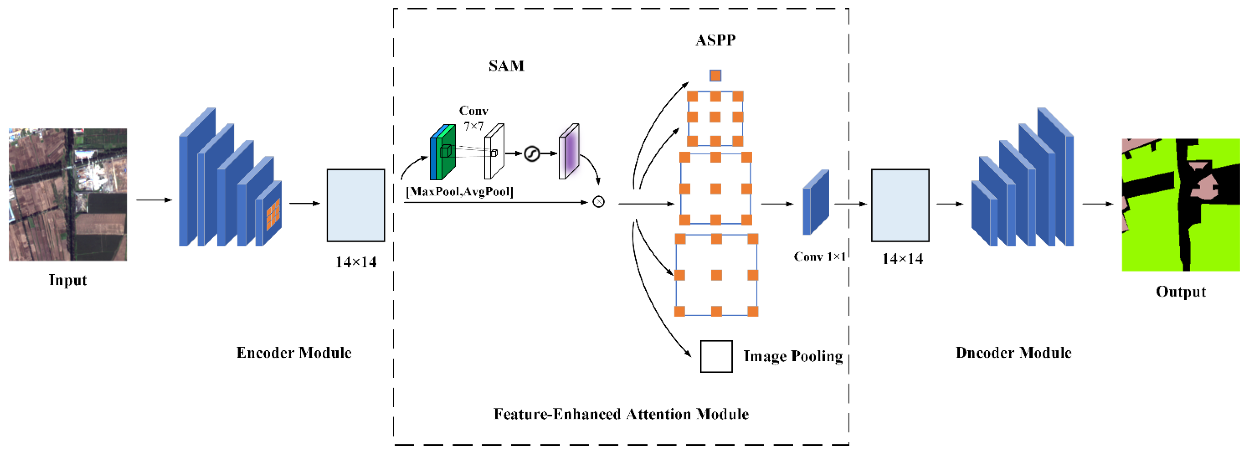
2.1. Network Architecture

Figure 1 shows the detailed model structure of VEDAM proposed in this paper. The proposed VEDAM is divided into three modules: the encoder module, the attention module, and the decoder module. The encoder module takes ResNet50 as the backbone network for feature extraction. Firstly, the image is convoluted, and the size of the feature map is continuously reduced through block1, block2, and block3 to extract effective features. Atrous convolution on the feature map is performed in block4. Following feature extraction, the feature map obtained by block4 is enhanced through the SAM in the attention module. In the decoder module, the ASPP operation is carried out, and the required spatial dimension is upsampled by bilinear interpolation to realize the semantic segmentation of satellite images.

2.2. Encoder Module

Our encoding network takes the improved ResNet50 [66] as the backbone network for feature extraction. First, the image is a convolution of 7 × 7, then the size of the feature map is continuously reduced through block1, block2, and block3 to extract effective features. At block4, atrous convolution is used to increase the receptive field. Finally, the size of the feature map obtained by the encoder module is 7 × 7 × 512, where 7 is the number of pixels and 512 is the number of channels of the feature map.

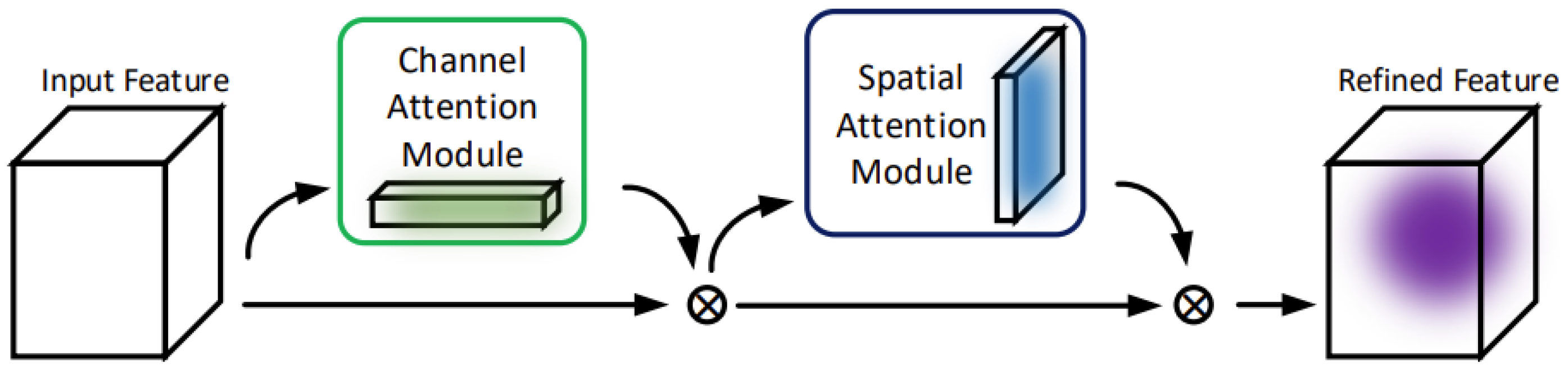
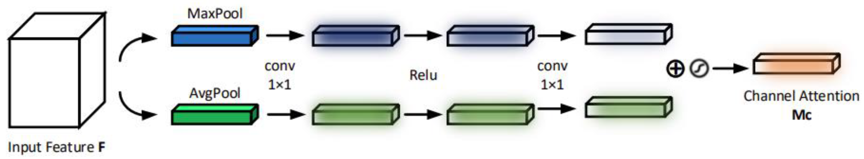
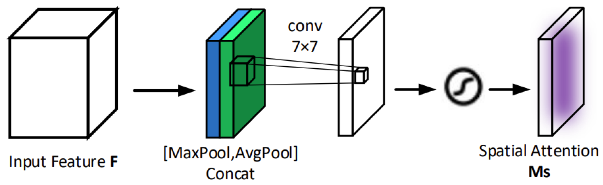
2.3. Feature-Enhanced Attention Module

After getting the feature map from the encoder module, the feature-enhanced attention module is implemented based on CBAM [67]. Compared with the Squeeze-and-Excitation (SE) module, the CBAM focuses on the feature relationship not only among channels but also among dimensions in space. As shown in Figure 2, the CBAM contains two parts: the Spatial Attention Module (SAM), targeting the feature relationship among dimensions in space; and the Channel Attention Module (CAM), the feature relationship among channels. Through the joint action of both modules, the network can recalibrate the features better.
The structure diagram of the CAM is shown in Figure 3. The feature recalibration process between channels is as follows: first, the input feature map is passed through the maximum pooling layer and the average pooling layer to get F m a x c and F a v g c , respectively. Then the outputs of the two are passed through the Multilayer Perceptron (MLP) with one hidden layer, in which the hidden activation size is set to C / r × 1 × 1 [67]. C is the number of channels and r is the reduction ratio to reduce parameter overhead. The MLP output features are added, and then the channel attention feature map is output through the sigmoid activation function. Finally, the channel attention feature map and the input feature map are multiplied to realize the feature recalibration of the feature map on the channel.
The channel attention is computed as [67]:
M c F = σ M L P A v g P o o l F + M L P M a x P o o l F = σ W 1 W 0 F a v g c + W 1 W 0 F m a x c ,
F is the input feature; σ is a sigmoid operation; AvgPool and MaxPool denote average pooling and maximum pooling, respectively; F a v g c and F m a x c denote average-pooled features and max-pooled features, respectively, where W 0 needs to be followed by the ReLU activation function, W 0 and W 1 represent the weight matrix of two convolution layers, M c is the channel recalibration feature.
The SAM is shown in Figure 4. The feature recalibration process between spaces is as follows: firstly, the input feature map is passed through the channel-based average pooling layer and maximum pooling layer; then the output results of the two are concatenated based on the channel features; and finally, through 7 × 7 convolution layer and sigmoid activation function generate spatial attention feature map and multiply the spatial attention feature map with the input feature map to realize the feature recalibration of the feature map in space.
The spatial attention is computed as [67]:
M s F = σ f 7 × 7 A v g P o o l F ; M a x P o o l F = σ f 7 × 7 F a v g s ; F m a x s ,
F is the input feature; σ is a sigmoid operation; AvgPool and MaxPool denote average pooling and maximum pooling, respectively; F a v g s and F m a x s denote average-pooled features and max-pooled features across the channel, respectively; f 7 × 7 represents a convolution operation with the filter size of 7 × 7 and M s is the spatial recalibration feature.
After the feature has been enhanced through SAM, the ASPP operation is carried out to make the input feature map 1 × 1 convolution and three 3 × 3 convolutions, when output_stride = 16, the atrous rate of convolution is rate = {6,12,18}. Output_stride is denoted by the ratio of input image spatial resolution to final output resolution. At the same time, the input feature map is pooled by global average pooling. The results obtained by four convolutions and one global average pooling are concatenated and 1 × 1 convolution.

2.4. Decoder Module

The final feature map with output_stride of 16 is finally obtained, after ResNet50 feature extraction, SAM feature enhancement, and ASPP capturing multi-scale context information. It is a challenge to reconstruct the original size segmentation graph from such a small feature map. Therefore, the feature map is upsampled on the decoder module. The ASPP output feature map is upsampled by bilinear interpolation with factor 16, and the size of the feature map is changed from 14 × 14 to 224 × 224 to get the final segmentation output.

3. Experimental Settings

In this section, the dataset used in the experiments is first introduced. Then, the experimental implementation details are explained. Finally, the evaluation criteria adopted are depicted.

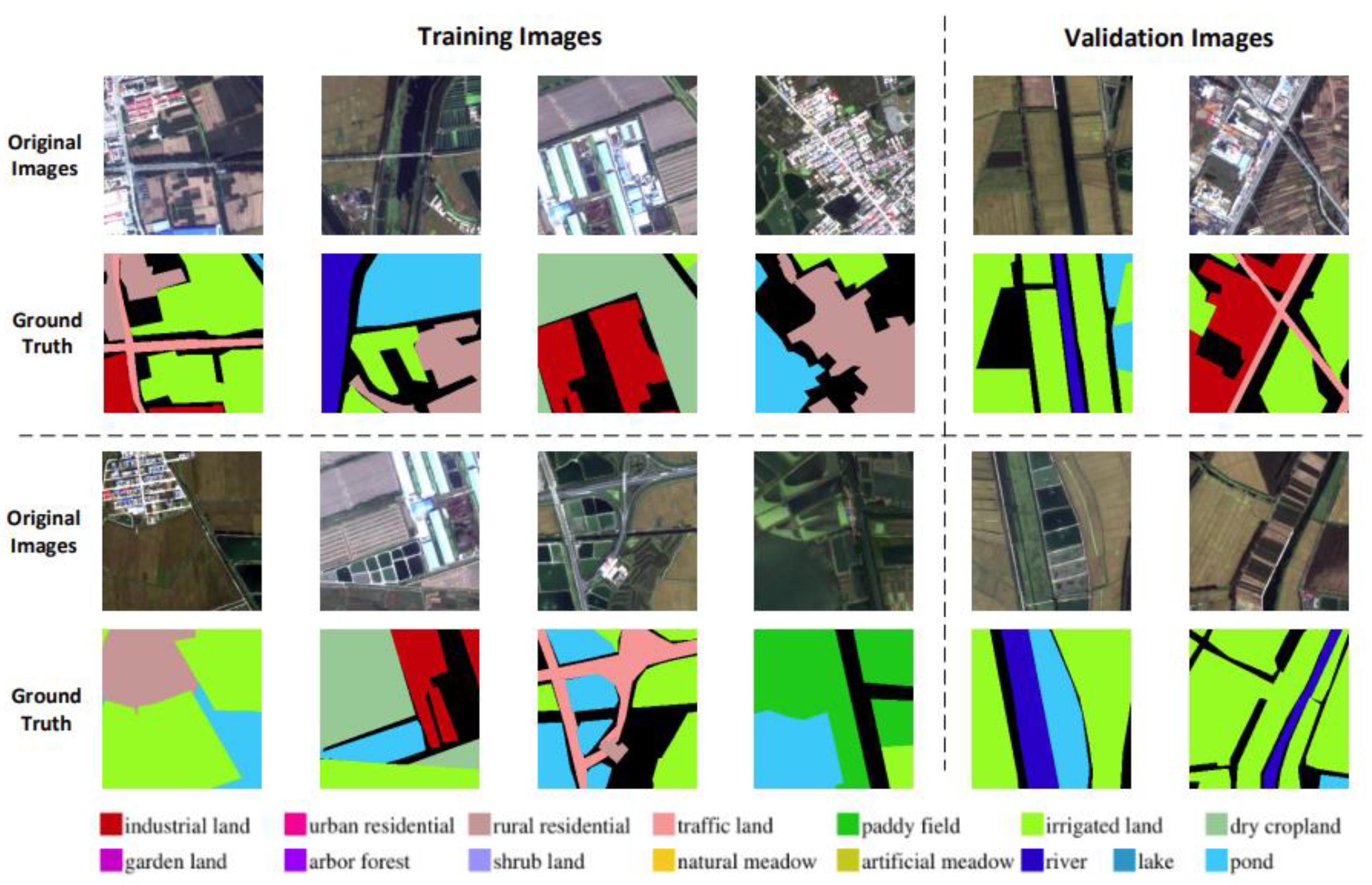
3.1. Gaofen Image Dataset (GID)

In this paper, the proposed VEDAM is tested and evaluated on the dataset GID, which is an open dataset [68]. It contains 150 high-quality Gaofen-2 (GF-2) images from more than 60 different cities in China, covering a geographical area of more than 50,000 km2. GID images have high intra-class diversity and low inter-class separability. Gf-2 satellite includes panchromatic images with a spatial resolution of 1 m and multispectral images with a spatial resolution of 4 m and image size of 6908 × 7300 pixels. Multispectral provides images in blue, green, red, and near-infrared bands. GID consists of a large-scale classification set and a fine land-cover classification set, both of which contain the original images and labeled ground truth. The fine land-cover classification set used in this experiment is composed of 15 fine classifications: paddy field, irrigated land, dry cropland, garden land, arbor forest, shrub land, natural meadow, artificial meadow, industrial land, urban residential, rural residential, traffic land, river, lake, and pond. The combination of paddy fields, irrigated land, dry cropland, garden land, arbor forest, shrub land, natural meadow, and artificial meadow is regarded as vegetation in our following discussion. Table 1 shows the vegetation classes in the GID Dataset. The total number of finally generated images is 37170, which is obtained by cutting the original images from 6800 × 7200 (h × w) to 224 × 224 with the cutting stride 112. A random set of 7170 cutting images is selected as the validation set (the validation set contains all classes and is evenly distributed). Figure 5 shows the sample images of training and validation images in the GID dataset.

3.2. Experimental Implementation Details

VEDAM is trained on a computer equipped with Intel Core i9-9900x and 64 GB of memory. The computer is equipped with two GPUs, type RTX2080ti, with 11 GB GPU memory. Because the training model requires a lot of GPU memory, the method in this paper uses 224 × 224 size images as input to the network. Adam [69] is an adaptive learning rate optimizer with high computational efficiency and low memory requirements. Therefore, this paper uses Adam optimizer to optimize the network and updates parameters. In addition, the network proposed in this paper uses NLLLoss as the loss function. When training VEDAM, the training epoch is set to 30 and the learning rate to 0.0001. The training batch size is 8.

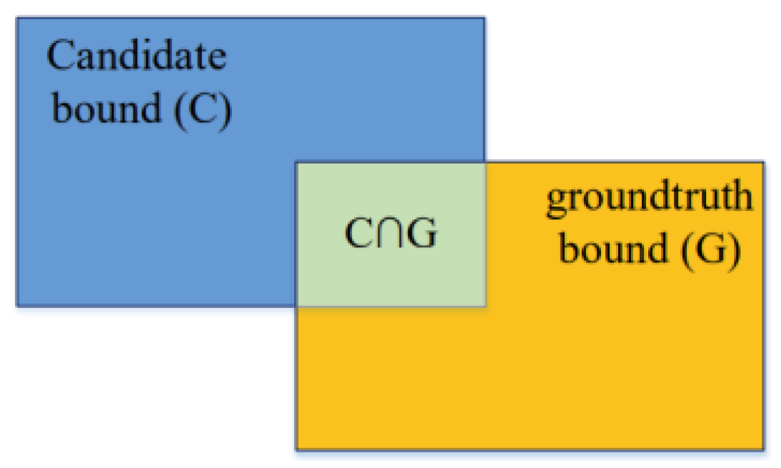
3.3. Comparative Methods and Evaluation Criteria

To verify the performance of VEDAM, it is compared with two representative deep learning network models, U-Net and SegNet, on the GID dataset under the same conditions. U-Net and SegNet have achieved satisfactory performance in different segmentation applications. The training settings are the same as VEDAM.
To evaluate the performance of the model comprehensively, seven widely used vegetation segmentation evaluation criteria are adopted. The one-vs-rest method is used to extend these binary classification criteria to multi-classification problems. The first 5 criteria are Accuracy [40], Recall [40], Precision [40], mIoU [65], and F-score [70], mIoU is expressed as follows:
m I o U = 1 k + 1 i = 0 k I o U = 1 k + 1 i = 0 k T P F N + F P + T P ,
where TP, FN, FP, and TN denote true positive, false negative, false positive, and true negative, respectively. k is the number of classes minus 1.
The sixth evaluation criterion is IoU, which is expressed in Figure 6, and calculated as follows:
I o U = a r e a C a r e a G a r e a C a r e a G = T P T P + F N + F P ,
area(C) represents the area of the candidate bound, and area(G) represents the area of the ground truth bound.
The seventh evaluation criterion is Kappa [71], which is expressed as follows:
K a p p a = A C C P 1 P ,
P = T P + F P T P + F N + F N + T N F P + T N N 2 ,
p represents the proportion of expected agreement between the ground truth and predictions with given class distributions [72]. N is the total number of pixels.

4. Experimental Results and Discussion

In this section, the overall performance of VEDAM is evaluated, then VEDAM is compared with two classical segmentation methods (U-Net and SegNet), and finally, the impact of the CBAM module on VEDAM is discussed. In each part, the 8 vegetation subclasses are classified into vegetation for discussion first, and then the performance of the model on the 8 vegetation subclasses is discussed in detail.

4.1. The Overall Results of the Classification Experiments

In this part, the experimental results of VEDAM on the GID dataset are discussed. As shown in Figure 7, through qualitative analysis, it can be seen that the vegetation is completely extracted. There are only some small errors, such as in Figure 7d, the small corner of the bottom is not correctly divided, in Figure 7f, there is an error in the segmentation of the middle joint, the rest of which is close to the ground truth. To verify the performance of VEDAM quantitatively, 8 out of all the 16 classes are discussed under vegetation (paddy fields, irrigated land, dry cropland, garden land, arbor forest, shrub land, natural meadow, and artificial meadow). Table 2 lists the Accuracy, Recall, Precision, F-score, IoU, mIoU, and Kappa of validation images of the GID dataset. Following, these 8 vegetation subclasses are discussed. Table 3 lists the Accuracy, Recall, Precision, F-score, IoU, mIoU, and Kappa of the 8 subclasses above mentioned.

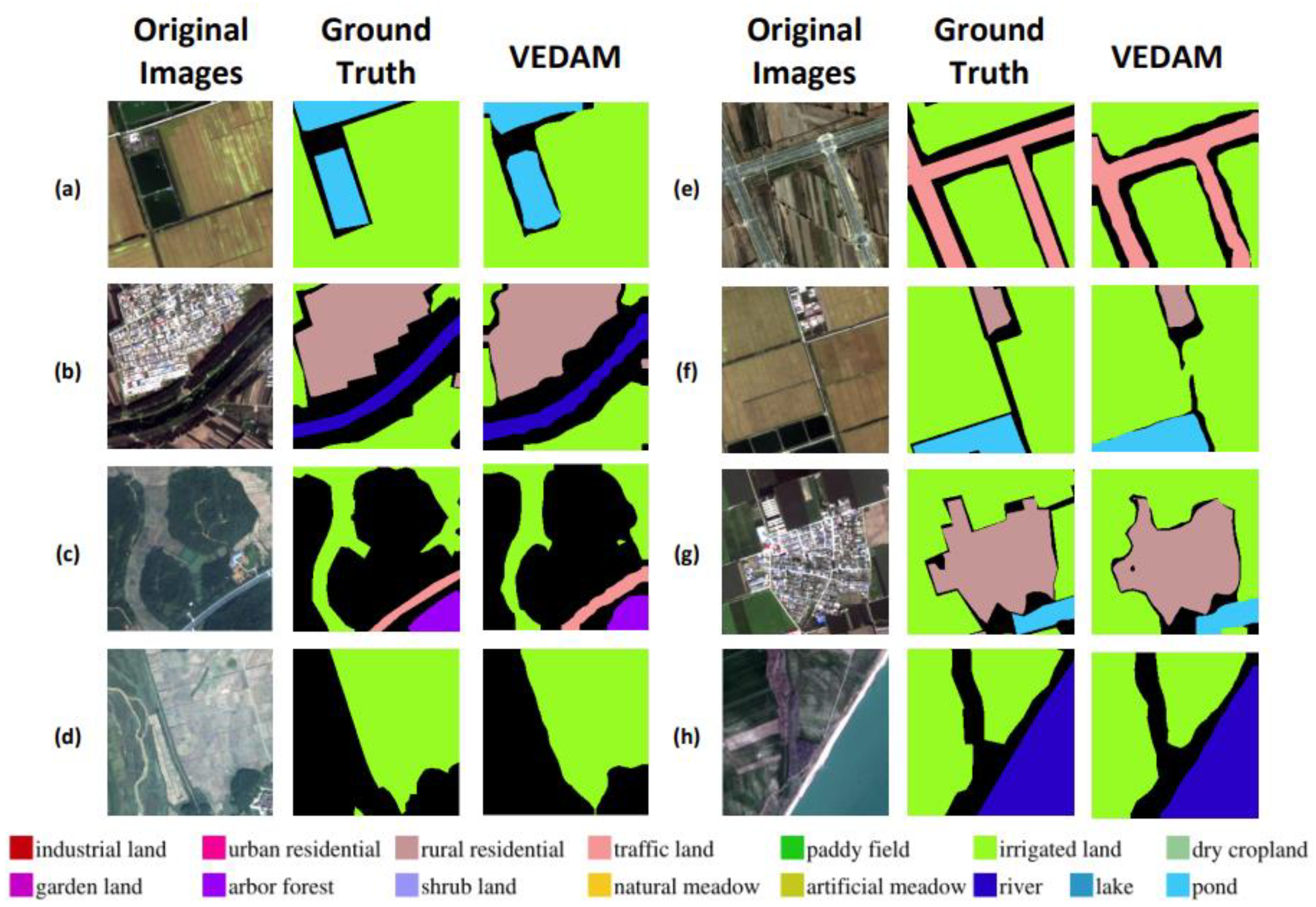
4.1.1. Performance on the GID Dataset

As shown in Table 2, VEDAM achieves good segmentation results in 9 classes. For all the classes of the GID dataset, the values of Accuracy, Recall, mIoU, and Kappa are higher than 90%, and Accuracy and Recall are even higher than 92%. As shown in bold in Table 2, it can be seen that the overall accuracy (Accuracy, Recall, Precision, F-score, and IoU) of the experimental results of vegetation classes are 98.15%, 97.46%, 97.37%, 97.42%, and 94.96%, respectively. This proves the excellent performance of VEDAM.

4.1.2. Performance in Vegetation Classes

It can be seen from Table 3 that the mIoU of experimental results within the vegetation classes can reach 91.36%. In the 8 vegetation subclasses, the values of Accuracy, Recall, Precision, IoU, and F-score are higher than 98%, 93%, 87%, 85%, and 91%, respectively.
In conclusion, the experimental results maintain the integrity of vegetation extraction, which shows that the model performs well in the task of vegetation extraction from high-resolution satellite images.

4.2. The Results of the Comparative Experiments

In this part, VEDAM is compared with two representative deep learning network models, namely, U-Net and SegNet, on the GID dataset under the same conditions.

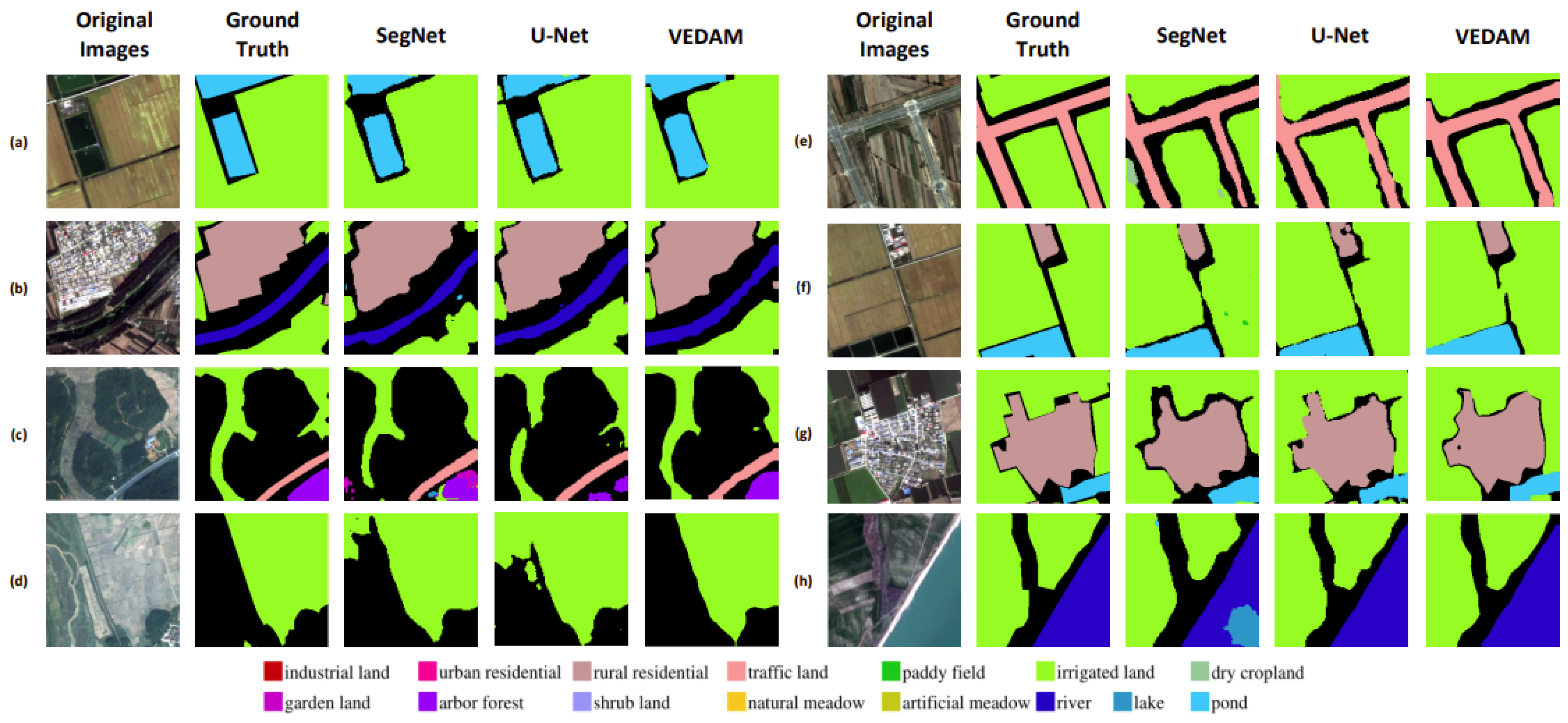
4.2.1. Performance on the GID Dataset

As shown in bold in Table 4, VEDAM achieves significantly better segmentation results in all nine classes than the other two. With the exception of Precision, which is slightly lower than the other two methods on traffic land, VEDAM outperforms U-Net and SegNet in all classes. For all classes of the GID dataset, Accuracy, Recall, and mIoU.

4.2.2. Performance in Vegetation Classes

Table 5 shows the experimental results of all methods on 8 vegetation subclasses. As shown in bold in Table 5, the segmentation effect of nearly all the vegetation subclasses is better than SegNet and U-Net. The F-score, obtained by VEDAM, exceeds 91%, much better than SegNet and U-Net. VEDAM achieves a mIoU value of 91.36% in 8 vegetation subclasses, which is 15.23% and 7.43% higher than SegNet and U-Net, respectively. Only on shrubland, the Precision of VEDAM is 5.03% lower than that of SegNet, but its Recall is 28.59% higher than that of SegNet. The reason is that the distribution of shrubland is discontinuous and there are fewer training samples. Overall, VEDAM is superior to the other two methods in the extraction of 8 vegetation subclasses.
Figure 8 shows the experimental results of all methods on the GID fine land-cover classification dataset. In general, the extraction results of VEDAM are almost consistent with the ground truth. Compared with the other two models, VEDAM has great advantages. As shown in the lower right corner of Figure 8c, there is an obvious misclassification problem in the extraction results of SegNet and U-Net. In Figure 8d, VEDAM obtains the smoothest segmentation result, while SegNet and U-Net to a certain extent of misclassification. In general, SegNet has a poor effect on edge segmentation between different classes, such as (a), (b), (e), and (g) in Figure 8. At the same time, there will be serious segmentation errors, such as (c), (d), and (h) in Figure 8. The segmentation effect of U-Net is slightly better than that of SegNet, and the segmentation effect is no less than that of VEDAM in (b), (g), and (h) of Figure 8, but there are still serious segmentation errors, such as (c) and (d) of Figure 8. Among the three models, the VEDAM has the best performance and the least segmentation errors of all the images, which is also consistent with the quantitative analysis results.

4.3. Effect of the CBAM

To verify the importance of the added SAM in the process of vegetation segmentation, the original model is compared with the model with different attention modules under the same training conditions. In the original model, the SAM added in VEDAM is deleted. In the comparison models, the CAM and CBAM are added in the same position as VEDAM. Validation experiments are conducted on the GID fine land-cover classification dataset. Table 6 shows the experimental results of the four models on the GID dataset.

4.3.1. Performance on the GID Dataset

As shown in bold in Table 6, VEDAM combined with the different attention modules achieves good segmentation results in 9 classes, of which VEDAM is better. In terms of the overall segmentation effect, mIoU and Kappa obtained by VEDAM are 91.57% and 94.50%, respectively, which are 1.08% and 0.71% higher than the VEDAM with SAM, 0.65% and 0.48% higher than the VEDAM-CAM, and 0.67% and 0.35% higher than the VEDAM-CBAM. As shown in bold italics in Table 6, it can be seen that Accuracy, Precision, F-score, and IoU of vegetation segmentation of the VEDAM have achieved the best results, reaching 98.15%, 97.37%, 97.42%, and 94.96%, respectively. VEDAM outperformed the other three methods in comparison. The results show that the VEDAM is better than other comparison methods in the segmentation of vegetation classes.

4.3.2. Performance in Vegetation Classes

Table 7 shows the experimental results of all methods in 8 classes within the vegetation. As shown in bold in Table 7, it can be seen that VEDAM has achieved higher Accuracy, Precision, F-score, IoU, and mIoU in most vegetation classes, especially mIoU reached 91.36%, which is 1.92% higher than the VEDAM without SAM, 3.13% higher than the VEDAM-CAM and 2.00% higher than the VEDAM-CBAM. This shows that the VEDAM method can effectively reduce the missing and misclassification of vegetation pixels and extract vegetation information more accurately.
Figure 9 shows the extraction results of the four methods on the GID dataset. It can be seen from the image that the models with the attention module achieve better extraction results, without large-area misclassification as SegNet and U-Net do. In contrast, the effect of edge segmentation between different classes in the original model is far from satisfactory. Due to the addition of the attention modules, VEDAM-CAM, VEDAM-CBAM, and VEDAM produce clearer boundaries between vegetation and non-vegetation. In the segmentation in the lower right corner of Figure 9g, the three comparison methods to a certain extent misclassification. Among them, the VEDAM without SAM misclassifies the background into vegetation, the VEDAM-CAM misclassifies the vegetation into the pond, and the VEDAM-CBAM misclassifies the pond into vegetation and background. The integrity of the extraction results of the VEDAM is much better than the other three comparison models. The vegetation results extracted from the original model and the other two network models inevitably have the problems of misclassification and omission.
In short, the added SAM can enhance the spatial feature information, by means of extracting the key details. It plays an important role in improving the performance of vegetation segmentation and ensuring its integrity of vegetation segmentation. Experiments show that the VEDAM has a good performance in vegetation segmentation.

4.4. Discussion

In this section, the misclassification of VEDAM and its potential application value is analyzed.

4.4.1. Analysis of Misclassification

VEDAM proposed in this paper has achieved remarkable results in the above comparative experiments, but due to the complex backgrounds, there is still a small amount of vegetation omission in the extraction process, which is unavoidable currently. There is a small amount of misclassification on the right side of Figure 9g and adhesion of vegetation segmentation in Figure 9f. Urban buildings, roads, pond, and vegetation constitute a complex background, which interferes with the perception of target features by the model, and, in turn, cause misclassification.

4.4.2. Potential application value of VEDAM

The semantic segmentation maps of high-resolution satellite images can be obtained by VEDAM, and the location, area, and species of urban vegetation can be obtained efficiently. Such information can not only provide valuable advice for urban decision-making, including on urban planning, livability, sustainability, and ecosystem services, but also accelerate urbanization, to help reduce pollution, maintain dust, mitigate urban heat island effect, flood control, carbon sequestration and promote sustainable urban development. Therefore, the efficient and accurate extraction of urban vegetation by VEDAM can become the key technology of modern urban planning and eco-environmental assessment.

5. Conclusions and Future Work

Satellite-terrestrial integrated IoT can capture rich ground observation information through satellite sensors and obtain high-space, high-spectral resolution satellite images, which can better reflect the land use land cover (LULC) on the ground, it provides the possibility of obtaining high-resolution satellite images. The use of remote sensing technology, especially satellite remote sensing, which is not restricted by ground conditions, makes it possible to obtain various valuable information in a convenient and timely manner. Extraction of urban vegetation from high-resolution satellite images can provide valuable suggestions for the decision-making of urban management.
For the purpose of vegetation extraction from high-resolution satellite images, a network called VEDAM is proposed in this paper. The network is based on the structure of the convolution model, in which atrous convolution is introduced to obtain more multi-scale context information. After feature extraction, SAM is used to enhance the spatial information of the extracted feature. The extracted features are further enhanced by ASPP and image pooling. VEDAM retains more detailed information, and the extraction result of vegetation information is more precise than that of the state-of-the-art models. In addition, on the GID fine land-cover classification dataset, VEDAM is compared with U-Net and SegNet. Experiments show that the VEDAM performs well qualitatively and quantitatively. VEDAM achieved the best mIoU of vegetation semantic segmentation (mIoU = 0.9136). Therefore, VEDAM is an effective vegetation extraction model with superior performance.
In future research, we will explore more vegetation subclasses as well as optimize the proposed model to better support decision-makers in sustainable urban planning and management.

Author Contributions

Conceptualization, B.Y. and M.Z.; methodology, B.Y. and M.Z.; validation, M.Z. and B.Y.; formal analysis, M.Z. and Y.X.; investigation, F.Z. and Z.S.; resources, Y.X.; writing original draft preparation, M.Z.; writing—review and editing, B.Y. and Y.X.; supervision, Y.X. and F.Z.; project administration, Y.X.; funding acquisition, B.Y. All authors have read and agreed to the published version of the manuscript.

Funding

This research received no external funding.

Data Availability Statement

Data is contained within the article.

Conflicts of Interest

The authors declare no conflict of interest.

References

  1. Liu, X.; Jia, M.; Zhou, M.; Wang, B.; Durrani, T.S. Integrated Cooperative Spectrum Sensing and Access Control for Cognitive Industrial Internet of Things. IEEE Internet Things J. 2023, 10, 1887–1896. [Google Scholar] [CrossRef]
  2. Jia, M.; Gao, Z.; Guo, Q.; Lin, Y.; Gu, X. Sparse Feature Learning for Correlation Filter Tracking Toward 5G-Enabled Tactile Internet. IEEE Trans. Ind. Inform. 2020, 16, 1904–1913. [Google Scholar] [CrossRef]
  3. Jia, M.; Zhang, X.; Sun, J.; Gu, X.; Guo, Q. Intelligent Resource Management for Satellite and Terrestrial Spectrum Shared Networking toward B5G. IEEE Wirel. Commun. 2020, 27, 54–61. [Google Scholar] [CrossRef]
  4. Taubenböck, H.; Weigand, M.; Esch, T.; Staab, J.; Wurm, M.; Mast, J.; Dech, S. A new ranking of the world’s largest citiesdo administrative units obscure morphological realities? Remote Sens. Environ. 2019, 232, 111353. [Google Scholar] [CrossRef]
  5. White, M.A.; Brunsell, N.; Schwartz, M.D. Vegetation Phenology in Global Change Studies. In Phenology: An Integrative Environmental Science. Tasks for Vegetation Science; Schwartz, M.D., Ed.; Springer: Dordrecht, The Netherlands, 2003; Volume 39. [Google Scholar] [CrossRef]
  6. Luo, Z.; Sun, O.J.; Ge, Q.; Xu, W.; Zheng, J. Phenological responses of plants to climate change in an urban environment. Ecol. Res. 2007, 22, 507–514. [Google Scholar] [CrossRef]
  7. Bidolakh, D.I.; Bilous, A.M.; Kuziovych, V.S. The accuracy of measuring the height of trees with the use of a quadrocopter. Ukr. J. For. Wood Sci. 2019, 10, 19–26. [Google Scholar] [CrossRef]
  8. Bidolakh, D.I. Geoinformation monitoring of green stands using remote sensing methods. Ann. For. Sci. 2020, 11, 4–14. [Google Scholar]
  9. Ozdarici-Ok, A.; Ok, A.O.; Schindler, K. Mapping of Agricultural Crops from Single High-Resolution Multispectral Images—Data-Driven Smoothing vs. Parcel-Based Smoothing. Remote Sens. 2015, 7, 5611–5638. [Google Scholar] [CrossRef] [Green Version]
  10. Yang, Y.; Newsam, S. Bag-of-visual-words and spatial extensions for land-use classification. In Proceedings of the 18th SIGSPATIAL International Conference on Advances in Geographic Information Systems, San Jose, CA, USA, 3–5 November 2010; pp. 270–279. [Google Scholar] [CrossRef]
  11. Gharineiat, Z.; Tarsha Kurdi, F.; Campbell, G. Review of automatic processing of topography and surface feature identification LiDAR data using machine learning techniques. Remote Sens. 2022, 14, 4685. [Google Scholar] [CrossRef]
  12. Camuffo, E.; Mari, D.; Milani, S. Recent Advancements in Learning Algorithms for Point Clouds: An Updated Overview. Sensors 2022, 22, 1357. [Google Scholar] [CrossRef]
  13. Zhang, X.; Du, S. Learning selfhood scales for urban land cover mapping with very-high-resolution satellite images. Remote Sens. Environ. 2016, 178, 172–190. [Google Scholar] [CrossRef]
  14. Melaas, E.K.; Wang, J.A.; Miller, D.L.; Friedl, M.A. Interactions between urban vegetation and surface urban heat islands: A case study in the boston metropolitan region. Environ. Res. Lett. 2016, 11, 054020. [Google Scholar] [CrossRef] [Green Version]
  15. Schreyer, J.; Geiß, C.; Lakes, T. TanDEM-X for Large-Area Modeling of Urban Vegetation Height: Evidence from Berlin, Germany. IEEE J. Sel. Top. Appl. Earth Obs. Remote Sens. 2016, 9, 1876–1887. [Google Scholar] [CrossRef] [Green Version]
  16. De, S.; Bhattacharyya, S.; Chakraborty, S.; Dutta, P. Hybrid Soft Computing for Multilevel Image and Data Segmentation; Springer: Berlin/Heidelberg, Germany, 2016. [Google Scholar] [CrossRef]
  17. Zhang, L.B.; Li, H. Region of interest detection based on visual attention and threshold segmentation in high spatial resolution remote sensing images. KSII Trans. Internet Inf. Syst. 2013, 7, 1843–1859. [Google Scholar] [CrossRef] [Green Version]
  18. Ghamisi, P.; Couceiro, M.S.; Ferreira, N.M.F.; Kumar, L. Use of Darwinian Particle Swarm Optimization technique for the segmentation of Remote Sensing images. In Proceedings of the 2012 IEEE International Geoscience and Remote Sensing Symposium, Munich, Germany, 22–27 July 2012; pp. 4295–4298. [Google Scholar] [CrossRef]
  19. Gaetano, R.; Masi, G.; Poggi, G.; Verdoliva, L.; Scarpa, G. Marker-Controlled Watershed-Based Segmentation of Multiresolution Remote Sensing Images. IEEE Trans. Geosci. Remote Sens. 2015, 53, 2987–3004. [Google Scholar] [CrossRef]
  20. Mylonas, S.K.; Stavrakoudis, D.G.; Theocharis, J.B.; Mastorocostas, P.A. Spectral-spatial classification of remote sensing images using a region-based GeneSIS Segmentation algorithm. In Proceedings of the 2014 IEEE International Conference on Fuzzy Systems (FUZZ-IEEE), Beijing, China, 6–11 July 2014; pp. 1976–1984. [Google Scholar] [CrossRef]
  21. Sellaouti, A. Méthode Collaborative de Segmentation et Classification d’objets à Partir d’images de Télédétection à Très Haute Résolution Spatiale. (Collaborative Method of Segmentation and Classification of Objects from Remote Sensing Images with Very High Spatial Resolution). Doctoral Dissertation, Tunis El Manar University, Tunis, Tunisie, 2014. [Google Scholar]
  22. Mylonas, S.K.; Stavrakoudis, D.G.; Theocharis, J.B. A GA-based sequential fuzzy segmentation approach for classification of remote sensing images. In Proceedings of the 2012 IEEE International Conference on Fuzzy Systems, Brisbane, QLD, Australia, 10–15 June 2012; pp. 1–8. [Google Scholar] [CrossRef]
  23. Michel, J.; Inglada, J. Multi-Scale Segmentation and Optimized Computation of Spatial Reasoning Graphs for Object Detection in Remote Sensing Images. In Proceedings of the IGARSS 2008-2008 IEEE International Geoscience and Remote Sensing Symposium, Boston, MA, USA, 7–11 July 2008; pp. III-431–III-434. [Google Scholar] [CrossRef]
  24. Ren, J.; Zeng, X.; McKee, D. Segmentation of multispectral images and prediction of CHI-A concentration for effective ocean colour remote sensing. In Proceedings of the 2015 IEEE International Geoscience and Remote Sensing Symposium (IGARSS), Milan, Italy, 26–31 July 2015; pp. 2303–2306. [Google Scholar] [CrossRef] [Green Version]
  25. Masi, G.; Gaetano, R.; Poggi, G.; Scarpa, G. Superpixel-based segmentation of remote sensing images through correlation clustering. In Proceedings of the 2015 IEEE International Geoscience and Remote Sensing Symposium (IGARSS), Milan, Italy, 26–31 July 2015; pp. 1028–1031. [Google Scholar] [CrossRef] [Green Version]
  26. Costa, W.S.; Fonseca, L.M.G.; Körting, T.S.; Simões, M.; Bendini, H.D.N.; Souza, R.C.M. Segmentation of optical remote sensing images for detecting homogeneous regions in space and time. In Proceedings of the XVIII Brazilian Symposium on GeoInformatics (GEOINFO 2017), Salvador, BA, Brazil, 4–6 December 2017; Unifacs: Salvador, BA, Brazil, 2017; Volume 18, pp. 40–51. [Google Scholar] [CrossRef]
  27. Chen, C.Y.; Feng, H.M.; Chen, H.C.; Jou, S.-M. Dynamic image segmentation algorithm in 3D descriptions of remote sensing images. Multimed. Tools Appl. 2016, 75, 9723–9743. [Google Scholar] [CrossRef]
  28. Szegedy, C.; Ioffe, S.; Vanhoucke, V.; Alemi, A. Inception-v4, Inception-ResNet and the Impact of Residual Connections on Learning. In Proceedings of the AAAI Conference on Artificial Intelligence, San Francisco, CA, USA, 4–9 February 2017; Volume 31. [Google Scholar] [CrossRef]
  29. Xu, Y.; Chen, Z.; Xie, Z.; Wu, L. Quality assessment of building footprint data using a deep autoencoder network. Int. J. Geogr. Inf. Sci. 2017, 31, 1929–1951. [Google Scholar] [CrossRef]
  30. Ren, S.; He, K.; Girshick, R.; Sun, J. Faster r-cnn: Towards real-time object detection with region proposal networks. Adv. Neural Inf. Process. Syst. 2015, 28, 91–99. [Google Scholar] [CrossRef] [Green Version]
  31. Kalayeh, M.M.; Shah, M. On Symbiosis of Attribute Prediction and Semantic Segmentation. IEEE Trans. Pattern Anal. Mach. Intell. 2021, 43, 1620–1635. [Google Scholar] [CrossRef]
  32. Mittal, S.; Tatarchenko, M.; Brox, T. Semi-Supervised Semantic Segmentation With High- and Low-Level Consistency. IEEE Trans. Pattern Anal. Mach. Intell. 2021, 43, 1369–1379. [Google Scholar] [CrossRef] [Green Version]
  33. Li, K.; Wu, Z.; Peng, K.-C.; Ernst, J.; Fu, Y. Guided Attention Inference Network. IEEE Trans. Pattern Anal. Mach. Intell. 2020, 42, 2996–3010. [Google Scholar] [CrossRef] [PubMed]
  34. Lin, D.; Huang, H. Zig-Zag Network for Semantic Segmentation of RGB-D Images. IEEE Trans. Pattern Anal. Mach. Intell. 2020, 42, 2642–2655. [Google Scholar] [CrossRef] [PubMed]
  35. Zhang, Y.; David, P.; Foroosh, H.; Gong, B. A Curriculum Domain Adaptation Approach to the Semantic Segmentation of Urban Scenes. IEEE Trans. Pattern Anal. Mach. Intell. 2020, 42, 1823–1841. [Google Scholar] [CrossRef] [Green Version]
  36. Gao, H.; Yuan, H.; Wang, Z.; Ji, S. Pixel Transposed Convolutional Networks. IEEE Trans. Pattern Anal. Mach. Intell. 2020, 42, 1218–1227. [Google Scholar] [CrossRef] [PubMed]
  37. Lin, G.; Liu, F.; Milan, A.; Shen, C.; Reid, I. RefineNet: Multi-Path Refinement Networks for Dense Prediction. IEEE Trans. Pattern Anal. Mach. Intell. 2020, 42, 1228–1242. [Google Scholar] [CrossRef] [PubMed]
  38. Wang, L.; Wang, L.; Lu, H.; Zhang, P.; Ruan, X. Salient Object Detection with Recurrent Fully Convolutional Networks. IEEE Trans. Pattern Anal. Mach. Intell. 2019, 41, 1734–1746. [Google Scholar] [CrossRef]
  39. Han, B.-B.; Zhang, Y.-T.; Pan, Z.-X.; Tai, X.-Q.; Li, F.-F. Residual dense spatial pyramid network for urban remote sensing image segmentation. J. Image Graph. 2020, 25, 2656. [Google Scholar]
  40. Li, W.; Zhao, W.; Zhong, H.; He, C.; Lin, D. Joint Semantic-geometric Learning for Polygonal Building Segmentation. In Proceedings of the AAAI Conference on Artificial Intelligence, Virtually, 2–9 February 2021; Volume 35, pp. 1958–1965. [Google Scholar] [CrossRef]
  41. Zheng, Z.; Zhong, Y.; Wang, J.; Ma, A. Foreground-aware relation network for geospatial object segmentation in high spatial resolution remote sensing imagery. In Proceedings of the IEEE/CVF Conference on Computer Vision and Pattern Recognition, Seattle, WA, USA, 13–19 June 2020; pp. 4096–4105. [Google Scholar]
  42. Ayhan, B.; Kwan, C. Application of Deep Belief Network to Land Cover Classification Using Hyperspectral Images. In Advances in Neural Networks-ISNN 2017; Cong, F., Leung, A., Wei, Q., Eds.; Lecture Notes in Computer Science; Springer: Cham, Switzerland, 2017; Volume 10261. [Google Scholar] [CrossRef]
  43. Yuan, M.; Ren, D.; Feng, Q.; Wang, Z.; Dong, Y.; Lu, F.; Wu, X. MCAFNet: A Multiscale Channel Attention Fusion Network for Semantic Segmentation of Remote Sensing Images. Remote Sens. 2023, 15, 361. [Google Scholar] [CrossRef]
  44. Li, L.; Zhang, W.; Zhang, X.; Emam, M.; Jing, W. Semi-Supervised Remote Sensing Image Semantic Segmentation Method Based on Deep Learning. Electronics 2023, 12, 348. [Google Scholar] [CrossRef]
  45. Li, H.; Qiu, K.; Chen, L.; Mei, X.; Hong, L.; Tao, C. SCAttNet: Semantic Segmentation Network With Spatial and Channel Attention Mechanism for High-Resolution Remote Sensing Images. IEEE Geosci. Remote Sens. Lett. 2021, 18, 905–909. [Google Scholar] [CrossRef]
  46. Tan, X.; Xiao, Z.; Wan, Q.; Shao, W. Scale Sensitive Neural Network for Road Segmentation in High-Resolution Remote Sensing Images. IEEE Geosci. Remote Sens. Lett. 2021, 18, 533–537. [Google Scholar] [CrossRef]
  47. Saltiel, T.M.; Dennison, P.E.; Campbell, M.J.; Thompson, T.R.; Hambrecht, K.R. Tradeoffs between UAS Spatial Resolution and Accuracy for Deep Learning Semantic Segmentation Applied to Wetland Vegetation Species Mapping. Remote Sens. 2022, 14, 2703. [Google Scholar] [CrossRef]
  48. Behera, T.K.; Bakshi, S.; Sa, P.K. A Lightweight Deep Learning Architecture for Vegetation Segmentation using UAV-captured Aerial Images. Sustain. Comput. Inform. Syst. 2023, 37, 100841. [Google Scholar] [CrossRef]
  49. Kwan, C.; Ayhan, B.; Budavari, B.; Lu, Y.; Perez, D.; Li, J.; Bernabe, S.; Plaza, A. Deep Learning for Land Cover Classification Using Only a Few Bands. Remote Sens. 2020, 12, 2000. [Google Scholar] [CrossRef]
  50. Kwan, C.; Gribben, D.; Ayhan, B.; Bernabe, S.; Plaza, A.; Selva, M. Improving Land Cover Classification Using Extended Multi-Attribute Profiles (EMAP) Enhanced Color, Near Infrared, and LiDAR Data. Remote Sens. 2020, 12, 1392. [Google Scholar] [CrossRef]
  51. Bhatnagar, S.; Gill, L.; Ghosh, B. Drone Image Segmentation Using Machine and Deep Learning for Mapping Raised Bog Vegetation Communities. Remote Sens. 2020, 12, 2602. [Google Scholar] [CrossRef]
  52. Badrinarayanan, V.; Kendall, A.; Cipolla, R. SegNet: A Deep Convolutional Encoder-Decoder Architecture for Image Segmentation. IEEE Trans. Pattern Anal. Mach. Intell. 2017, 39, 2481–2495. [Google Scholar] [CrossRef]
  53. Yang, M.-D.; Tseng, H.-H.; Hsu, Y.-C.; Tsai, H.P. Semantic Segmentation Using Deep Learning with Vegetation Indices for Rice Lodging Identification in Multi-date UAV Visible Images. Remote Sens. 2020, 12, 633. [Google Scholar] [CrossRef] [Green Version]
  54. Wu, C.; Ju, B.; Xiong, N.; Yang, G.; Wu, Y.; Yang, H.; Huang, J.; Xu, Z. U-net super-neural segmentation and similarity calculation to realize vegetation change assessment in satellite imagery. arXiv 2019, arXiv:1909.04410. [Google Scholar] [CrossRef]
  55. Ronneberger, O.; Fischer, P.; Brox, T. U-net: Convolutional networks for biomedical image segmentation. In Proceedings of the International Conference on Medical Image Computing and Computer-Assisted Intervention, Munich, Germany, 5–9 October 2015; Springer: Berlin/Heidelberg, Germany, 2015; pp. 234–241. [Google Scholar] [CrossRef] [Green Version]
  56. Heryadi, Y.; Irwansyah, E.; Miranda, E.; Soeparno, H.; Herlawati; Hashimoto, K. The Effect of Resnet Model as Feature Extractor Network to Performance of DeepLabV3 Model for Semantic Satellite Image Segmentation. In Proceedings of the 2020 IEEE Asia-Pacific Conference on Geoscience, Electronics and Remote Sensing Technology (AGERS), Jakarta, Indonesia, 7–8 December 2020; pp. 74–77. [Google Scholar] [CrossRef]
  57. Zeng, F.; Yang, B.; Zhao, M.; Xing, Y.; Ma, Y. MASANet: Multi-Angle Self-Attention Network for Semantic Segmentation of Remote Sensing Images. Teh. Vjesn. 2022, 29, 1567–1575. [Google Scholar] [CrossRef]
  58. Kwan, C.; Gribben, D.; Ayhan, B.; Li, J.; Bernabe, S.; Plaza, A. An Accurate Vegetation and Non-Vegetation Differentiation Approach Based on Land Cover Classification. Remote Sens. 2020, 12, 3880. [Google Scholar] [CrossRef]
  59. Chen, L.-C.; Papandreou, G.; Schroff, F.; Adam, H. Rethinking atrous convolution for semantic image segmentation. arXiv 2017, arXiv:1706.05587. [Google Scholar] [CrossRef]
  60. Wu, Q.; Luo, F.; Wu, P.; Wang, B.; Yang, H.; Wu, Y. Automatic Road Extraction from High-Resolution Remote Sensing Images Using a Method Based on Densely Connected Spatial Feature-Enhanced Pyramid. IEEE J. Sel. Top. Appl. Earth Obs. Remote Sens. 2021, 14, 3–17. [Google Scholar] [CrossRef]
  61. Ni, Z.-L.; Bian, G.-B.; Wang, G.-A.; Zhou, X.-H.; Hou, Z.-G.; Chen, H.-B.; Xie, X.-L. Pyramid Attention Aggregation Network for Semantic Segmentation of Surgical Instruments. In Proceedings of the AAAI Conference on Artificial Intelligence, New York, NY, USA, 7–12 February 2020; Volume 34, pp. 11782–11790. [Google Scholar] [CrossRef]
  62. Zhong, Z.; Lin, Z.Q.; Bidart, R.; Hu, X.; Daya, I.B.; Li, Z.; Zheng, W.-S.; Li, J.; Wong, A. Squeeze-and-attention networks for semantic segmentation. In Proceedings of the IEEE/CVF Conference on Computer Vision and Pattern Recognition, Seattle, WA, USA, 13–19 June 2020; pp. 13065–13074. [Google Scholar] [CrossRef]
  63. Chen, L.; Tian, X.; Chai, G.; Zhang, X.; Chen, E. A New CBAM-P-Net Model for Few-Shot Forest Species Classification Using Airborne Hyperspectral Images. Remote Sens. 2021, 13, 1269. [Google Scholar] [CrossRef]
  64. Chen, Y.; Zhang, X.; Chen, W.; Li, Y.; Wang, J. Research on Recognition of Fly Species Based on Improved RetinaNet and CBAM. IEEE Access 2020, 8, 102907–102919. [Google Scholar] [CrossRef]
  65. Chen, L.-C.; Zhu, Y.; Papandreou, G.; Schroff, F.; Adam, H. Encoderdecoder with atrous separable convolution for semantic image segmentation. In Proceedings of the European Conference on Computer Vision (ECCV), Munich, Germany, 8–14 September 2018; pp. 801–818. [Google Scholar] [CrossRef]
  66. He, K.; Zhang, X.; Ren, S.; Sun, J. Deep Residual Learning for Image Recognition. In Proceedings of the 2016 IEEE Conference on Computer Vision and Pattern Recognition (CVPR), Las Vegas, NV, USA, 27–30 June 2016; pp. 770–778. [Google Scholar] [CrossRef] [Green Version]
  67. Woo, S.; Park, J.; Lee, J.Y.; Kweon, I.S. Cbam: Convolutional block attention module. In Proceedings of the European Conference on Computer Vision (ECCV), Munich, Germany, 8–14 September 2018; pp. 3–19. [Google Scholar] [CrossRef]
  68. Tong, X.-Y.; Xia, G.-S.; Lu, Q.; Shen, H.; Li, S.; You, S.; Zhang, L. Landcover classification with high-resolution remote sensing images using transferable deep models. Remote Sens. Environ. 2020, 237, 111322. [Google Scholar] [CrossRef] [Green Version]
  69. Kingma, D.P.; Ba, J. Adam: A method for stochastic optimization. arXiv 2014, arXiv:1412.6980. [Google Scholar] [CrossRef]
  70. Zang, Y.; Wang, C.; Yu, Y.; Luo, L.; Yang, K.; Li, J. Joint Enhancing Filtering for Road Network Extraction. IEEE Trans. Geosci. Remote Sens. 2017, 55, 1511–1525. [Google Scholar] [CrossRef]
  71. Kraemer, H.C. Kappa coefficient. Wiley StatsRef Stat. Ref. Online 2014, 1–4. [Google Scholar] [CrossRef]
  72. El Amin, A.M.; Liu, Q.; Wang, Y. Zoom out CNNs features for optical remote sensing change detection. In Proceedings of the 2017 2nd International Conference on Image, Vision and Computing (ICIVC), Chengdu, China, 2–4 June 2017; pp. 812–817. [Google Scholar] [CrossRef]
Figure 1. Model structure of VEDAM.
Electronics 12 01215 g001
Figure 2. CBAM network structure diagram.
Electronics 12 01215 g002
Figure 3. Network structure of the CAM.
Electronics 12 01215 g003
Figure 4. Network structure of the SAM.
Electronics 12 01215 g004
Figure 5. Sample images of training and validation images in the GID dataset.
Electronics 12 01215 g005
Figure 6. IoU calculation diagram.
Electronics 12 01215 g006
Figure 7. Visualization of segmentation results of VEDAM on the GID Dataset, (a–h) represents the visualization results of randomly selected samples.
Electronics 12 01215 g007
Figure 8. Visualization of segmentation results of SegNet, U-Net, and VEDAM on the GID Dataset, (ah) represents the visualization results of randomly selected samples.
Electronics 12 01215 g008
Figure 9. Visualization of segmentation results of VEDAM combined with different attention modules on the GID dataset, (a–h) represents the visualization results of randomly selected samples.
Electronics 12 01215 g009
Table 1. The 8 vegetation subclasses in the GID dataset.
Vegetation
ForestFarmlandMeadow
garden landarbor
forest
shrub landpaddy fieldirrigated landdry croplandnatural meadowartificial meadow
Table 2. Experiment results of the GID dataset by VEDAM.
Back
Ground
Industria
Land
Urban
Residential
Rural
Residential
Traffic
Land
VegetationRiverLakePond
ACC0.96440.99610.99360.99490.99300.98150.99880.99940.9987
Recall0.94680.95990.96220.92230.93140.97460.98900.98920.9725
Precision0.95620.95330.96520.93390.84870.97370.97880.97920.9611
F-score0.95150.95660.96370.92810.88820.97420.98390.98420.9668
IoU0.90750.91680.92990.96580.79880.94960.96830.96880.9357
mIoU0.9157
Kappa0.9450
Table 3. Experiment results of the GID dataset for 8 vegetation subclasses by VEDAM.
Paddy
Field
Irrigated
Land
Dry
Cropland
Garden
Plot
Arbor
Woodland
Shrub
Land
Natural
Grassland
Artificial
Grassland
ACC0.99820.98840.99840.99930.99620.99960.99910.9996
Recall0.96560.97460.95480.93370.96970.97170.95820.9750
Precision0.96870.97450.96790.92480.96630.87350.95900.9408
F-score0.96710.97450.96130.92920.96800.91990.95860.9576
IoU0.93640.95030.92540.86780.93800.85180.92050.9186
mIoU0.9136
Table 4. Comparison results of U-Net, SegNet, and VEDAM on the GID dataset.
Back
Ground
Industrial
Land
Urban
Residential
Rural
Residential
Traffic
Land
VegetationRiverLakePond
ACCU-Net0.94740.99350.98940.99310.99220.97000.99830.99850.9979
SegNet0.92290.99010.98230.99000.98980.95480.99500.99470.9965
VEDAM0.96440.99610.99360.99490.99300.98150.99880.99940.9987
RecallU-Net0.91240.92560.94530.91800.87200.97210.98110.95130.9478
SegNet0.91250.83620.95360.80650.79830.91920.90860.91720.9247
VEDAM0.94680.95990.96220.92230.93140.97460.98900.98920.9725
PrecisionU-Net0.94290.92990.93650.89240.86860.94550.97350.96220.9470
SegNet0.88210.93770.86240.90340.85180.95260.95530.81070.9043
VEDAM0.95620.95330.96520.93390.84870.97370.97880.97920.9611
F-scoreU-Net0.92740.92770.94080.90510.87030.95860.97730.95670.7474
SegNet0.89700.88410.90570.85220.82410.93560.93140.86070.9144
VEDAM0.95150.95660.96370.92810.88820.97420.98390.98420.9668
IoUU-Net0.86460.86520.88830.82660.77450.92050.95550.91710.9001
SegNet0.81330.79220.82770.74250.70090.87900.87150.75540.8422
VEDAM0.90750.91680.92990.86580.79880.94960.96830.96880.9357
mIoUU-Net0.8792
SegNet0.8027
VEDAM0.9157
KappaU-Net0.9129
SegNet0.8727
VEDAM0.9450
Kappa is more than 90%, and Accuracy and Recall are even higher than 92%. As shown in bold italics in Table 4, it can be seen that the Accuracy of vegetation extraction by VEDAM is as high as 98.15%, 1.15% higher than U-Net, and 2.67% higher than SegNet. Recall, Accuracy, and F-score of VEDAM are higher than 97%, 5.54%, 2.11%, and 3.86% higher than SegNet, respectively, higher than U-Net by 0.25%, 2.82%, and 1.56%. The IoU of VEDAM is 94.96%, 7.06% higher than that of SegNet and 2.91% higher than that of U-Net. The results show that VEDAM is superior to the other two methods in the extraction of the vegetation class.
Table 5. Comparison results of U-Net, SegNet, and VEDAM on the GID dataset for 8 vegetation subclasses.
Paddy
Field
Irrigated
Land
Dry
Cropland
Garden
Plot
Arbor
Woodland
Shrub
Land
Natural
Grassland
Artificial
Grassland
ACCU-Net0.99720.98180.99730.99890.99300.99920.99840.9986
SegNet0.99510.96790.99160.99840.99050.99920.99770.9987
VEDAM0.99820.98840.99840.99930.99620.99960.99910.9996
RecallU-Net0.94770.97280.93990.87110.95960.92740.93840.9669
SegNet0.88660.91400.63990.75790.94490.68580.91520.8823
VEDAM0.96560.97460.95480.93370.96970.97170.95820.9750
PrecisionU-Net0.94830.94870.93130.88230.92380.73960.91360.8005
SegNet0.92870.94320.93750.87780.89870.92380.87800.8670
VEDAM0.96870.97450.96790.92480.96630.87350.95900.9408
F-scoreU-Net0.94800.96060.93560.87670.94130.82290.92580.8759
SegNet0.90710.92830.96070.81350.92120.78720.89620.8760
VEDAM0.96710.97450.96130.92920.96800.91990.95860.9576
IoUU-Net0.90110.92420.87900.78040.88910.69910.86190.7792
SegNet0.83000.86630.61380.68560.85400.64910.81200.7794
VEDAM0.93640.95030.92540.86780.93800.85180.92050.9186
mIoUU-Net0.8393
SegNet0.7613
VEDAM0.9136
Table 6. Comparison results of VEDAM combined with different attention modules on the GID dataset.
Back
Ground
Industrial
Land
Urban
Residential
Rural
Residential
Traffic
Land
VegetationRiverLakePond
ACCVEDAM0.96440.99610.99360.99490.99300.98150.99880.99940.9987
VEDAM w/o SAM0.96000.99560.99290.99390.99240.97890.99850.99930.9983
VEDAM-CAM0.96130.99580.99320.99460.99290.97940.99870.99940.9983
VEDAM-CBAM0.96210.99580.99320.99490.99310.97970.99860.99930.9980
RecallVEDAM0.94680.95990.96220.92230.93140.97460.98900.98920.9725
VEDAM w/o SAM0.93100.95090.95920.93230.93600.97770.99030.97280.9658
VEDAM-CAM0.95030.94340.95730.91180.89460.97120.97560.98310.9632
VEDAM-CBAM0.94130.95780.96870.93400.91870.97290.99100.98830.9222
PrecisionVEDAM0.95620.95330.96520.93390.84870.97370.97880.97920.9611
VEDAM w/o SAM0.95920.95120.96070.90130.83150.96380.97020.98660.9526
VEDAM-CAM0.94490.96250.96560.93550.87120.97120.98800.98560.9547
VEDAM-CBAM0.95520.94950.95570.92330.86090.97040.97090.97440.9778
F-scoreVEDAM0.95150.95660.96370.92810.88820.97420.98390.98420.9668
VEDAM w/o SAM0.94490.95110.95990.91650.88070.97070.98020.97960.9592
VEDAM-CAM0.94760.95290.96140.92350.88270.97120.98180.98430.9590
VEDAM-CBAM0.94820.95360.96220.92860.88890.97170.98090.98130.9492
IoUVEDAM0.90750.91680.92990.86580.79880.94960.96830.96880.9357
VEDAM w/o SAM0.89560.90670.92300.84590.78680.94300.96110.96010.9216
VEDAM-CAM0.90050.91000.92570.85790.79010.94400.96420.96920.9212
VEDAM-CBAM0.90150.91140.92710.86680.80000.94490.96250.96330.9033
mIoUVEDAM0.9157
VEDAM w/o SAM0.9049
VEDAM-CAM0.9092
VEDAM-CBAM0.9090
KappaVEDAM0.9450
VEDAM w/o SAM0.9379
VEDAM-CAM0.9402
VEDAM-CBAM0.9415
Table 7. Comparison results of VEDAM combined with different attention modules on 8 vegetation subclasses on the GID dataset.
Paddy
Field
Irrigated
Land
Dry
Cropland
Garden
Plot
Arbor
Woodland
Shrub
Land
Natural
Grassland
Artificial
Grassland
ACCVEDAM0.99820.98840.99840.99930.99620.99960.99910.9996
VEDAM w/o SAM0.99810.98710.99830.99930.99530.99940.99890.9995
VEDAM-CAM0.99780.98710.99840.99910.99580.99920.99900.9994
VEDAM-CBAM0.99790.98700.99850.99900.99550.99940.99900.9996
RecallVEDAM0.96560.97460.95480.93370.96970.97170.95820.9750
VEDAM w/o SAM0.96010.97960.94940.92840.97400.97560.94620.9614
VEDAM-CAM0.94140.97030.95780.93920.96810.97090.95130.9635
VEDAM-CBAM0.96680.96690.96750.94880.97640.98460.95790.9701
PrecisionVEDAM0.96870.97450.96790.92480.96630.87350.95900.9408
VEDAM w/o SAM0.97060.96450.96730.91930.94740.78590.95090.9351
VEDAM-CAM0.97730.97280.96360.88360.96080.72540.95290.9128
VEDAM-CBAM0.95530.97570.95970.85950.94800.77680.95080.9485
F-scoreVEDAM0.96710.97450.96130.92920.96800.91990.95860.9576
VEDAM w/o SAM0.96530.97200.95830.92390.96050.87050.94850.9480
VEDAM-CAM0.95900.97150.96070.91050.96450.83040.95210.9375
VEDAM-CBAM0.96100.97130.96350.90190.96200.86840.95430.9592
IoUVEDAM0.93640.95030.92540.86780.93800.85180.92050.9186
VEDAM w/o SAM0.93290.94550.91990.85850.92400.77070.90210.9012
VEDAM-CAM0.92120.94470.92430.83580.93130.71000.90860.8823
VEDAM-CBAM0.92500.94420.92970.82140.92680.76740.91260.9215
mIoUVEDAM0.9136
VEDAM w/o SAM0.8944
VEDAM-CAM0.8823
VEDAM-CBAM0.8936
Disclaimer/Publisher’s Note: The statements, opinions and data contained in all publications are solely those of the individual author(s) and contributor(s) and not of MDPI and/or the editor(s). MDPI and/or the editor(s) disclaim responsibility for any injury to people or property resulting from any ideas, methods, instructions or products referred to in the content.

